Relativistic coupled-cluster theory of nuclear spin-dependent parity non-conservation

Abstract

We have developed a relativistic coupled-cluster theory to incorporate nuclear spin-dependent interaction Hamiltonians perturbatively. In this theory, the coupled-cluster operators in the electronic sector are defined as tensor operators of rank one and we introduce suitable diagrammatic representations. For properties calculations, the electronic part is first calculated and later coupled to the nuclear spin part. The method is ideal to calculate parity violating nuclear spin-dependent electric dipole transition amplitudes, $E1_{\rm PNC}^{\rm NSD}$, of heavy atoms. To validate the proposed method the $E1_{\rm PNC}^{\rm NSD}$ of the transition $6\;^{2}S_{1/2}\rightarrow 7\;^{2}S_{1/2}$ in ¹³³Cs is calculated for selected MBPT diagrams and compared with the results from our theory.

I Introduction

Experimental observation of nuclear spin dependent (NSD) parity non-conservation (PNC) is a signature of nuclear anapole moment (NAM) zeldovich-58 . It is the most dominant NSD-PNC effect among three possible sources. The other two are: combination of hyperfine and nuclear spin-independent PNC; and spin-dependent $Z$ exchange between electrons and nucleus. To date, the most precise atomic PNC measurement, of atomic Cs, has provided the only experimental evidence of NAM wood-97 . One major hurdle to a clear observation of nuclear anapole moment is the large nuclear spin-independent (NSI) signal, which overwhelms the NSD signature. However, proposed experiments with single Ba⁺ ion fortson-93 could probe PNC in the $s_{1/2}-d_{5/2}$ transition, where the NSI component is zero. This could then provide an unambiguous observation of NSD-PNC and NAM in particular. The ongoing experiments with atomic Ytterbium tsigutkin-09 is another possibility, the $6s^{2}\;{}^{1}S_{0}-6s5d\;^{3}D_{2}$ transition, to observe NSD-PNC with minimal mixture from the NSI component. One crucial input, which is also the source of large uncertainty, to extract the value of NAM and nuclear weak charge in NSI-PNC is the input from atomic theory calculations. In the case of isotope chain measurements, like in Yb, the PNC observable is a ratio. Atomic theory contributions then cancel and parameters can be extracted without atomic theory calculations. However, results from atomic theory calculations are important in estimating the expected value of PNC transition amplitudes and extracting NAM does require results from atomic theory. For these reasons, it is important to employ reliable and accurate many-body theory in the atomic theory calculations.

Recently, atomic theory calculations have investigated the NSD-PNC of Ba⁺ and Ra⁺ using the atomic many-body perturbation theory (MBPT) sahoo-11 . Another recent work reports the theoretical estimate of the NSD-PNC observable of Yb dzuba-11a and the calculations are based on the CI-MBPT method dzuba-96 . There is also an earlier work on NSD-PNC of Yb using the same method porsev-00 . Very recently, the CI-MBPT method is used to to calculate the NSD-PNC observables of Ba⁺, Yb⁺ and Ra⁺ dzuba-11b . Besides the methods mentioned, earlier works on Ba⁺ geetha-98 and Yb angom-99 used configuration interaction (CI). To date, coupled-cluster theory (CCT) considered as one of the most reliable and accurate many-body theory has not been used in the NSD-PNC calculations. The difficulty of developing a suitable theory stems from the complications of dealing with the nuclear spin dependent interaction. In a previous paper of ours we reported the development of a relativistic coupled-cluster (RCC) theory to incorporate nuclear spin-dependent interaction in a consistent scheme mani-11b . In this work we provide elaborate details of the theory and touch upon related subtle issues.

The coupled-cluster (CC) theorycoester-58 ; coester-60 is one of the most reliable many-body theory to incorporate electron correlation in atomic calculations. In atomic physics, the relativistic coupled-cluster (RCC) theory has been used extensively in atomic properties calculations, for example, hyperfine structure constants pal-07 ; sahoo-09 , electric dipole moments nataraj-08 ; latha-09 , and electromagnetic transition properties thierfelder-09 ; sahoo-09a . In atomic PNC calculations too, RCC is the preferred theory and several groups have used it to calculate NSI-PNC of atoms wansbeek-08 ; pal-09 ; porsev-10 . However, the calculations in Ref. wansbeek-08 are entirely based on RCC with a variation we refer to as perturbed RCC (PRCC), where as the calculations in Ref. pal-09 ; porsev-10 are based on sum over states with CC wave functions. Naturally, the former incorporates electron correlation more precisely than the later approach.

In this work we provide a detailed explanation on the approach we have adopted to incorporate nuclear spin-dependent interaction Hamiltonian as a perturbation in RCC theory. In Section. II, we give a very short account of RCC theory to serve as a quick reference. We then give the details of our formulation to represent a NSD interaction perturbed CC operator in Section. III. PRCC equations of closed-shell and one-valence systems is derived in this section. To simplify angular factor calculations, the calculations in the electronic sector is separated out. Based on this the calculation of NSD-PNC observable, in the electronic sector, is described in Section. IV. Next section, Section. V, describes the coupling of results from the electronic sector with the nuclear spin. This completes the theoretical development and then, the correctness of theory is verified in Section. VI. For which, we use MBPT results and calculate the NSD-PNC of the $6\;^{2}S_{1/2}\rightarrow 7\;^{2}S_{1/2}$ transition in Cs. We then conclude and the angular factors of all the diagrams in the linearized PRCC are given in the Appendix.

II Brief review of RCC

For $N$-electron atoms or ions the Dirac-Coulomb Hamiltonian, appropriate to account for relativistic effects, is

$$H^{\rm DC}=\sum_{i=1}^{N}\left[c\bm{\alpha}_{i}\cdot\mathbf{p}_{i}+(\beta_{i}-1)c^{2}-V_{N}(r_{i})\right]+\sum_{i<j}\frac{1}{r_{ij}},$$ (1)

where $\bm{\alpha}_{i}$ and $\beta$ are the Dirac matrices, $\mathbf{p}$ is the linear momentum, $V_{N}(r)$ is the nuclear Coulomb potential and last term is the electron-electron Coulomb interactions. For one-valence systems it satisfies the eigen value equation

$$H^{\rm DC}|\Psi_{v}\rangle=E_{v}|\Psi_{v}\rangle,$$ (2)

where $|\Psi_{v}\rangle$ and $E_{v}$ are the atomic state and energy respectively. In the CC method, the atomic state is expressed in terms of $T$ and $S$, the closed-shell and one-valence cluster operators respectively, as

$$|\Psi_{v}\rangle=e^{T^{(0)}}\left[1+S^{(0)}\right]|\Phi_{v}\rangle,$$ (3)

where $|\Phi_{v}\rangle$ is the one-valence Dirac-Fock reference state. It is obtained by adding an electron to the closed-shell reference state, $|\Phi_{v}\rangle=a^{\dagger}_{v}|\Phi_{0}\rangle$. In the coupled-cluster singles doubles (CCSD) approximation $T^{(0)}=T^{(0)}_{1}+T^{(0)}_{2}$ and are the solutions of the nonlinear coupled equations

$$\langle\Phi^{p}_{a}|\bar{H}_{\rm N}|\Phi_{0}\rangle=0,$$ (4a)

$$\langle\Phi^{pq}_{ab}|\bar{H}_{\rm N}|\Phi_{0}\rangle=0,$$ (4b)

where $\bar{H}_{\rm N}=e^{-T^{(0)}}H_{\rm N}e^{T^{(0)}}$ is the similarity transformed Hamiltonian and the normal order Hamiltonian $H_{\rm N}=H-\langle\Phi_{0}|H|\Phi_{0}\rangle$. The states $|\Phi^{p}_{a}\rangle$ and $|\Phi^{pq}_{ab}\rangle$ are the singly and doubly excited determinants, respectively and $abc\ldots$ ($pqr\ldots$) denote occupied (virtual) orbitals. The details of the derivation are given in Ref. mani-09 . Like in $T^{(0)}$, the one-valence cluster operator $S^{(0)}$ in the CCSD approximation is $S^{(0)}=S^{(0)}_{1}+S^{(0)}_{2}$. And these are the solutions of

$$\langle\Phi_{v}^{p}|\bar{H}_{N}\!+\!\{\mathchoice{\vbox{\hbox to0.0pt{\kern 5.00002pt\kern 4.56248pt\hbox{\vrule width=0.50003pt,height=0.0pt,depth=2.15277pt\vrule width=13.02663pt,height=0.0pt,depth=0.50003pt\vrule width=0.50003pt,height=0.0pt,depth=2.15277pt}\hss}\vskip 2.15277pt\vskip 6.83331pt}}{\vbox{\hbox to0.0pt{\kern 5.00002pt\kern 4.56248pt\hbox{\vrule width=0.50003pt,height=0.0pt,depth=2.15277pt\vrule width=13.02663pt,height=0.0pt,depth=0.50003pt\vrule width=0.50003pt,height=0.0pt,depth=2.15277pt}\hss}\vskip 2.15277pt\vskip 6.83331pt}}{\vbox{\hbox to0.0pt{\kern 5.00002pt\kern 3.19374pt\hbox{\vrule width=0.50003pt,height=0.0pt,depth=2.15277pt\vrule width=9.19162pt,height=0.0pt,depth=0.50003pt\vrule width=0.50003pt,height=0.0pt,depth=2.15277pt}\hss}\vskip 2.15277pt\vskip 4.78333pt}}{\vbox{\hbox to0.0pt{\kern 5.00002pt\kern 2.28123pt\hbox{\vrule width=0.50003pt,height=0.0pt,depth=2.15277pt\vrule width=7.60829pt,height=0.0pt,depth=0.50003pt\vrule width=0.50003pt,height=0.0pt,depth=2.15277pt}\hss}\vskip 2.15277pt\vskip 3.41666pt}}\bar{H}_{N}S^{(0)}\}|\Phi_{v}\rangle = E_{v}^{\rm att}\langle\Phi_{v}^{p}|S^{(0)}_{1}|\Phi_{v}\rangle,$$ (5a)

$$\langle\Phi_{va}^{pq}|\bar{H}_{N}+\{\mathchoice{\vbox{\hbox to0.0pt{\kern 5.00002pt\kern 4.56248pt\hbox{\vrule width=0.50003pt,height=0.0pt,depth=2.15277pt\vrule width=13.02663pt,height=0.0pt,depth=0.50003pt\vrule width=0.50003pt,height=0.0pt,depth=2.15277pt}\hss}\vskip 2.15277pt\vskip 6.83331pt}}{\vbox{\hbox to0.0pt{\kern 5.00002pt\kern 4.56248pt\hbox{\vrule width=0.50003pt,height=0.0pt,depth=2.15277pt\vrule width=13.02663pt,height=0.0pt,depth=0.50003pt\vrule width=0.50003pt,height=0.0pt,depth=2.15277pt}\hss}\vskip 2.15277pt\vskip 6.83331pt}}{\vbox{\hbox to0.0pt{\kern 5.00002pt\kern 3.19374pt\hbox{\vrule width=0.50003pt,height=0.0pt,depth=2.15277pt\vrule width=9.19162pt,height=0.0pt,depth=0.50003pt\vrule width=0.50003pt,height=0.0pt,depth=2.15277pt}\hss}\vskip 2.15277pt\vskip 4.78333pt}}{\vbox{\hbox to0.0pt{\kern 5.00002pt\kern 2.28123pt\hbox{\vrule width=0.50003pt,height=0.0pt,depth=2.15277pt\vrule width=7.60829pt,height=0.0pt,depth=0.50003pt\vrule width=0.50003pt,height=0.0pt,depth=2.15277pt}\hss}\vskip 2.15277pt\vskip 3.41666pt}}\bar{H}_{N}S^{(0)}\}|\Phi_{v}\rangle = E_{v}^{\rm att}\langle\Phi_{va}^{pq}|S^{(0)}_{2}|\Phi_{v}\rangle,$$ (5b)

where $E_{v}^{\rm att}=E_{v}-E_{0},$ is the attachment energy of the valence electron. In our previous work mani-10 , we provide details of the derivation.

III Perturbed CC wave function

Time independent perturbation theory is the standard procedure to incorporate external perturbations or additional interactions in atomic many-body calculations. However, a basic requirement of perturbative calculations is a complete set of intermediate atomic states, which is non-trivial to generate. The perturbed CC method latha-08 ; mani-09 ; sahoo-08 , on the other hand, implicitly accounts for all the possible intermediate states. In this work, we consider the perturbation as the nuclear spin-dependent parity non-conserving (PNC) interaction

$$H_{\rm PNC}^{\rm NSD}=\frac{G_{\rm F}\mu^{\prime}_{W}}{\sqrt{2}}\sum_{i}\bm{\alpha}_{i}\cdot\mathbf{I}\rho_{\rm{N}}(r),$$ (6)

where $\mu^{\prime}_{W}$ is the weak nuclear moment of the nucleus and $\rho_{\rm N}(r)$ is the nuclear density. The weak nuclear moment is expressed in terms of the neutron and proton numbers $\mu^{\prime}_{W}=2(ZC_{1p}+NC_{1n})$, where $C_{1p}$ and $C_{1n}$ are respectively the vector electron and the axial vector nucleon coupling coefficients. There are two complications arising from the nuclear spin operator $I$ in $H_{\rm PNC}^{\rm NSD}$. First, the cluster operators in the electron space are rank one operators, and second, the atomic states in the one-valence sector are eigenstates of total angular momentum $\mathbf{F}=\mathbf{I}+\mathbf{J}$. Both of these are relatively simple to incorporate at lower order MBPT calculations, however, implementing these in non-perturbative theory like RCC is nontrivial. Accordingly, the method we have developed and implemented in the current work are very different from our previous works latha-08 ; mani-09 . The other simplifying feature of the previous works is, the methods developed were for closed-shell systems where the total electronic angular momentum $\mathbf{J}=0$.

With the PNC interaction, the total atomic Hamiltonian is

$$H_{\rm A}=H^{\rm DC}+\lambda H_{\rm PNC}^{\rm NSD},$$ (7)

where $\lambda$ is the perturbation parameter. As $H_{\rm PNC}^{\rm NSD}$ mixes atomic states of opposite parities, the eigenvalue equation is modified to

$$H_{\rm A}|\widetilde{\Psi}_{v}\rangle=E_{v}|\widetilde{\Psi}_{v}\rangle.$$ (8)

Note that the first order energy correction $E^{1}=\langle\Psi_{0}|H_{\rm PNC}^{\rm NSD}|\Psi_{0}\rangle=0$ as $H_{\rm PNC}^{\rm NSD}$ is an odd parity interaction Hamiltonian. This is taken into account while writing the above eigenvalue equation. Here $|\widetilde{\Psi}_{v}\rangle$ are the mixed parity atomic states and to first order in perturbation

$$|\widetilde{\Psi}_{v}\rangle=|\Psi_{v}\rangle+\sum_{I}|\Psi_{I}\rangle\frac{\langle\Psi_{I}|H_{\rm PNC}^{\rm NSD}|\Psi_{v}\rangle}{E_{v}-E_{I}}.$$ (9)

If $|\Psi_{v}\rangle$ and $|\Psi_{w}\rangle$ are atomic states of same parity, then the $H_{\rm PNC}^{\rm NSD}$ induced electric dipole ($E1$ ) transition amplitude is

$$E1_{\rm PNC}^{\rm NSD}=\langle\widetilde{\Psi}_{w}|\!|\mathbf{D}|\!|\widetilde{\Psi}_{v}\rangle,$$ (10)

where $\mathbf{D}$ is the dipole operator. The perturbation expression in Eq. (9) require a complete set of intermediate atomic states $|\Psi_{I}\rangle$. This, as mentioned at the beginning of the section, is non-trivial to obtain in atomic many-body calculations. Summation over intermediate states is circumvented when $E1_{\rm PNC}^{\rm NSD}$ is calculated with CC atomic states. For this define a new set of cluster operators $\mathbf{T}^{(1)}$, which unlike $T^{(0)}$ connects the reference state to opposite parity states. This is the result of incorporating one order of $H_{\rm PNC}^{\rm NSD}$ and for this reason we refer to $\mathbf{T}^{(1)}$ as the perturbed cluster operators. Although hyperfine states are natural to $H_{\rm PNC}^{\rm NSD}$, cluster operator $\mathbf{T}^{(1)}$ is defined to operate only in the electronic space and is a rank one operator. So, the mixed parity atomic state in RCC is

$$|\widetilde{\Psi}_{0}\rangle=e^{T^{(0)}+\lambda\mathbf{T}^{(1)}\cdot\mathbf{I}}|\Phi_{0}\rangle.$$ (11)

The scalar product with the nuclear spin $\mathbf{I}$ in the exponent restores $\mathbf{T}^{(1)}$ to the correct form of the wave operator. At this point it is convenient to separate out the electronic part of the interaction Hamiltonian

$${\mathbf{H}}_{\rm elec}^{\rm NSD}=\frac{G_{\rm F}\mu^{\prime}_{W}}{\sqrt{2}}\sum_{i}\vec{\alpha}_{i}\rho_{\rm{N}}(r),$$ (12)

which operates only in the electronic space, so that

$$H_{\rm PNC}^{\rm NSD}={\mathbf{H}}_{\rm elec}^{\rm NSD}\cdot\mathbf{I}.$$ (13)

The remaining part of this section describe how to arrive at a consistent representation of $\mathbf{T}^{(1)}$ and extension of the method to one-valence systems, where $\mathbf{S}^{(1)}$ are the perturbed cluster operators.

III.1 MBPT wavefunctions

To define the multipole and parity selection rules of $T^{(1)}$, we examine the second order MBPT wave function with $H_{\rm PNC}^{\rm NSD}$ as one of the perturbations. From the generalized Bloch equation lindgren-85 , the total wave operator is sahoo-11

$$\Omega_{v}=\sum_{n=1}^{\infty}\Omega_{v,0}^{(n)}+\sum_{n=1}^{\infty}\Omega_{v,1}^{(n)}.$$ (14)

Here $\Omega_{v,0}^{(n)}$ has $n$ orders of residual Coulomb interaction, where as $\Omega_{v,1}^{(n)}$ has one order of $H_{\rm PNC}^{\rm NSD}$ and $n$ orders of residual Coulomb interaction. Following which the mixed parity state

$$|\widetilde{\Psi}_{v}\rangle=|\Psi_{v}\rangle+|\bar{\Psi}_{v}\rangle=\sum_{n=1}^{\infty}\Omega_{v,0}^{(n)}|\Phi_{v}\rangle+\sum_{n=1}^{\infty}\Omega_{v,1}^{(n)}|\Phi_{v}\rangle,$$ (15)

where $|\bar{\Psi}_{v}\rangle$ is the opposite parity component arising from the $H_{\rm PNC}^{\rm NSD}$. The first order wave function is then,

$$|\widetilde{\Psi}_{v}^{1}\rangle=|\Psi_{v}^{1}\rangle+|\bar{\Psi}_{v}^{1}\rangle=\left[1+\Omega^{(1)}_{v,0}\right]|\Phi_{v}\rangle+\Omega^{(1)}_{v,1}|\Phi_{v}\rangle.$$ (16)

Although, notation wise $\Omega_{v,1}^{(1)}$ seem first order, it is second order in perturbation: one order each in residual Coulomb interaction and $H_{\rm PNC}^{\rm NSD}$. For model space consisting of same parity states

$$\left[\Omega_{v,1}^{(1)},H_{0}\right]P=QH_{\rm PNC}^{\rm NSD}\Omega_{v,0}P+QV_{\rm res}\Omega_{v,1}^{(0)}P.$$ (17)

Here, and $P$ and $Q$ are the projection operators of the model and complementary spaces, respectively, $H_{0}$ is the Dirac-Fock Hamiltonian, $V_{\rm res}$ is the residual Coulomb interaction and the zeroth order mixed parity wave operator

$$\Omega_{v,1}^{(0)}P=Q\frac{1}{E_{v}^{0}-H_{0}}QH_{\rm PNC}^{\rm NSD}P.$$ (18)

Using $\Omega_{v,1}^{(1)}$ and $\Omega_{v,0}^{(1)}$, we may compute $E1_{\rm PNC}$ to third order in perturbation, the details of which are discussed in Ref. sahoo-11 .

III.2 Perturbed cluster operator representation

The expression of $\Omega_{v,1}^{(1)}$ and associated selection rules are what we need to arrive at a consistent description of $T^{(1)}$.

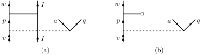
Figure 1: Second order MBPT diagram where interaction Hamiltonian $H_{\rm PNC}^{\rm NSD}$ operates on the particle state $p$. (a) Diagrammatic representation of $H_{\rm PNC}^{\rm NSD}$ in the electronic and nuclear spin space. (b) Diagrammatic representation within the electronic space only where the PNC interaction Hamiltonian is $H_{\rm elec}^{\rm NSD}$. Line terminated with square represents the PNC interaction.

In Fig. 1(a) we show an MBPT wave function diagram of $\Omega_{v,1}^{(1)}$ arising from the second term in Eq. (18). The algebraic expression of the diagram is

$$\frac{G_{\rm F}\mu^{\prime}_{W}}{\sqrt{2}}\sum_{p}|wqI\rangle\frac{\langle wI|\bm{\alpha}\cdot\mathbf{I}\rho_{\rm{N}}(r)|pI\rangle\langle pqI|V_{\rm res}|vaI\rangle}{(\epsilon_{w}-\epsilon_{p})(\epsilon_{v}+\epsilon_{a}-\epsilon_{p}-\epsilon_{q})},$$ (19)

where $\epsilon_{i}$ are the orbital energies. The states $|\cdots I\rangle$ represent uncoupled atomic states comprising of electronic and nuclear states.

Figure 2: Angular reduction of the second order MBPT diagram. The remnant angular momentum diagram on the right is representative of the multipole structure of PRCC double excitation cluster operators $T_{2}^{(1)}$ and $S_{2}^{(1)}$.

On closer examination, the component of $H_{\rm PNC}^{\rm NSD}$ which operates in the nuclear subspace is diagonal. So, for further calculations, we separate out the matrix elements in the electronic subspace and combine with the nuclear part at the end of the calculations. For the MBPT diagram considered earlier Fig. 1(a), the electronic part is as shown in Fig. 1(b). The corresponding algebraic expression is

$$\frac{G_{\rm F}\mu^{\prime}_{W}}{\sqrt{2}}\sum_{p}\frac{\langle w|\bm{\alpha}\rho_{\rm{N}}(r)|p\rangle\langle pq|V|va\rangle}{(\epsilon_{w}-\epsilon_{p})(\epsilon_{v}+\epsilon_{a}-\epsilon_{p}-\epsilon_{q})}.$$ (20)

Details of the angular reduction when electronic state is coupled with the nuclear state are discussed in the later sections of the paper. Like wise, the perturbed cluster operators $\mathbf{T}^{(1)}$, as defined earlier operate only in the electronic. For this consider the angular part of the matrix elements in Eq. (20), the diagrammatic representation is shown in Fig. 2. The angular diagrams are based on the conventions used in Lindgren and Morrison lindgren-85 and the same is followed in the remaining of the paper while referring to angular momentum diagrams. In the figure, the angular diagram on the right hand side indicates the multipole structure of the $T^{(1)}_{2}$ and like the electron-electron Coulomb interaction

$$\mathbf{T}^{(1)}_{2}=\sum_{abpq}\sum_{l,k_{2}}\tau_{ab}^{pq}(l,k_{2})\{\mathbf{C}_{l}(\hat{r}_{1})\mathbf{C}_{k_{2}}(\hat{r}_{2})\}^{1},$$ (21)

where $\mathbf{C}_{i}$ are c-tensor operators and $\{\cdots\}^{1}$ indicates the two c-tensor operators couple to a rank one tensor operator. Following general rules of coupling tensor operators, the rank of the tensor operators must satisfy the triangular conditions $|j_{w}-j_{v}|\leqslant l\leqslant(j_{w}+j_{v})$, $|j_{a}-j_{q}|\leqslant k_{2}\leqslant(j_{a}+j_{q})$ and $|l-k_{2}|\leqslant 1\leqslant(l+k_{2})$. Effectively, $\mathbf{T}^{(1)}$ is a rank one operator in the electronic subspace and forms a scalar operator after coupling with $\mathbf{I}$. The other important difference from the $T^{(0)}$ is the parity selection rule at the vertices. The combined parities at the vertices are opposite $(-1)^{l_{w}+l_{v}}=-(-1)^{l_{a}+l_{q}}$ . After a similar analysis, the singles operator is

$$\mathbf{T}^{(1)}_{1}=\sum_{ap}\tau_{a}^{p}\mathbf{C}_{1}(\hat{r}).$$ (22)

Based on the multipole structures, the perturbed cluster operators are diagrammatically represented as shown in Fig. 3. For the doubles $\mathbf{T}^{(1)}_{2}$, to indicate the multipole structure, an additional line is added to the interaction line.

III.3 Closed-shell systems

The mixed parity states, eigenstates of $H_{\rm A}$, in the perturbed relativistic coupled-cluster (PRCC) is as given in Eq. (11). However, as $H_{\rm PNC}^{\rm NSD}$ is considered to first order only, it is sufficient to consider up to linear terms in the expansion of $e^{\lambda\mathbf{T}^{(1)}\cdot\mathbf{I}}$. The PRCC atomic state is then

$$|\widetilde{\Psi}_{0}\rangle=e^{T^{(0)}}\left[1+\lambda\mathbf{T}^{(1)}\cdot\mathbf{I}\right]|\Phi_{0}\rangle.$$ (23)

The cluster operator $\mathbf{T}^{(1)}$, as described earlier, incorporates ${\mathbf{H}}_{\rm elec}^{\rm NSD}$ to first order and residual Coulomb interaction to all order.

Figure 3: Diagrammatic representation of the single and double excitation perturbed cluster operators in closed shell and one-valence sectors. The extra line in the $T_{2}^{(1)}$ and $S_{2}^{(1)}$ is to indicate the multipole structure of the operators.

The closed-shell equivalent of Eq. (8), the mixed parity eigenvalue equation, is

$$\left(H^{\rm DC}+\lambda{\mathbf{H}}_{\rm elec}^{\rm NSD}\cdot\mathbf{I}\right)|\widetilde{\Psi}_{0}\rangle=E_{0}|\widetilde{\Psi}_{0}\rangle.$$ (24)

From the definition of the coupled-cluster mixed parity state in Eq. (23), the eigen value equation in terms of the coupled-cluster wavefunction is

$$\left(H^{\rm DC}+\lambda{\mathbf{H}}_{\rm elec}^{\rm NSD}\cdot\mathbf{I}\right)e^{T^{(0)}}\left[1+\lambda\mathbf{T}^{(1)}\cdot\mathbf{I}\right]|\Phi_{0}\rangle$$

$$=E_{0}e^{T^{(0)}}\left[1+\lambda\mathbf{T}^{(1)}\cdot\mathbf{I}\right]|\Phi_{0}\rangle.$$ (25)

In terms of $H_{N}$, defined earlier, the eigenvalue equation is simplified to

$$\left(H_{\rm N}+\lambda{\mathbf{H}}_{\rm elec}^{\rm NSD}\right)e^{T^{(0)}}\left[1+\lambda\mathbf{T}^{(1)}\cdot\mathbf{I}\right]|\Phi_{0}\rangle$$

$$=\Delta E_{0}e^{T^{(0)}}\left[1+\lambda\mathbf{T}^{(1)}\cdot\mathbf{I}\right]\Phi_{0}\rangle,$$ (26)

where $\Delta E_{0}=E_{0}-\langle\Phi_{0}|H|\Phi_{0}\rangle$ is the closed-shell correlation energy. Retaining terms which are first-order in $\lambda$, we get

$$\left[H_{\rm N}\mathbf{T}^{(1)}\cdot\mathbf{I}+{\mathbf{H}}_{\rm elec}^{\rm NSD}\cdot\mathbf{I}\right]e^{T^{(0)}}|\Phi_{0}\rangle=\Delta E_{0}\mathbf{T}^{(1)}\cdot\mathbf{I}e^{T^{(0)}}|\Phi_{0}\rangle.$$ (27)

From here on, for simplicity, we drop the nuclear spin operator $\mathbf{I}$ and work only in the electronic space. At a later stage of the calculations the electronic part is coupled with the nuclear spin. Operating with $e^{-T^{(0)}}$ and projecting on singly and doubly excited states $\langle\Phi^{p}_{a}|$ and $\langle\Phi^{pq}_{ab}|$, respectively, we get the CC equations for singles and doubles perturbed cluster amplitudes as

$$\langle\Phi^{p}_{a}|\{\mathchoice{\vbox{\hbox to0.0pt{\kern 0.0pt\kern 4.56248pt\hbox{\vrule width=0.50003pt,height=0.0pt,depth=4.30554pt\vrule width=12.3788pt,height=0.0pt,depth=0.50003pt\vrule width=0.50003pt,height=0.0pt,depth=4.30554pt}\hss}\vskip 2.15277pt\vskip 6.83331pt}}{\vbox{\hbox to0.0pt{\kern 0.0pt\kern 4.56248pt\hbox{\vrule width=0.50003pt,height=0.0pt,depth=4.30554pt\vrule width=12.3788pt,height=0.0pt,depth=0.50003pt\vrule width=0.50003pt,height=0.0pt,depth=4.30554pt}\hss}\vskip 2.15277pt\vskip 6.83331pt}}{\vbox{\hbox to0.0pt{\kern 0.0pt\kern 3.19374pt\hbox{\vrule width=0.50003pt,height=0.0pt,depth=4.30554pt\vrule width=8.72516pt,height=0.0pt,depth=0.50003pt\vrule width=0.50003pt,height=0.0pt,depth=4.30554pt}\hss}\vskip 2.15277pt\vskip 4.78333pt}}{\vbox{\hbox to0.0pt{\kern 0.0pt\kern 2.28123pt\hbox{\vrule width=0.50003pt,height=0.0pt,depth=4.30554pt\vrule width=7.0894pt,height=0.0pt,depth=0.50003pt\vrule width=0.50003pt,height=0.0pt,depth=4.30554pt}\hss}\vskip 2.15277pt\vskip 3.41666pt}}\bar{\mathbf{H}}_{\rm N}\mathbf{T}^{(1)}\}|\Phi_{0}\rangle=-\langle\Phi^{p}_{a}|\bar{\mathbf{H}}_{\rm elec}^{\rm NSD}|\Phi_{0}\rangle,$$ (28a)

$$\langle\Phi^{pq}_{ab}|\{\mathchoice{\vbox{\hbox to0.0pt{\kern 0.0pt\kern 4.56248pt\hbox{\vrule width=0.50003pt,height=0.0pt,depth=4.30554pt\vrule width=12.3788pt,height=0.0pt,depth=0.50003pt\vrule width=0.50003pt,height=0.0pt,depth=4.30554pt}\hss}\vskip 2.15277pt\vskip 6.83331pt}}{\vbox{\hbox to0.0pt{\kern 0.0pt\kern 4.56248pt\hbox{\vrule width=0.50003pt,height=0.0pt,depth=4.30554pt\vrule width=12.3788pt,height=0.0pt,depth=0.50003pt\vrule width=0.50003pt,height=0.0pt,depth=4.30554pt}\hss}\vskip 2.15277pt\vskip 6.83331pt}}{\vbox{\hbox to0.0pt{\kern 0.0pt\kern 3.19374pt\hbox{\vrule width=0.50003pt,height=0.0pt,depth=4.30554pt\vrule width=8.72516pt,height=0.0pt,depth=0.50003pt\vrule width=0.50003pt,height=0.0pt,depth=4.30554pt}\hss}\vskip 2.15277pt\vskip 4.78333pt}}{\vbox{\hbox to0.0pt{\kern 0.0pt\kern 2.28123pt\hbox{\vrule width=0.50003pt,height=0.0pt,depth=4.30554pt\vrule width=7.0894pt,height=0.0pt,depth=0.50003pt\vrule width=0.50003pt,height=0.0pt,depth=4.30554pt}\hss}\vskip 2.15277pt\vskip 3.41666pt}}\bar{\mathbf{H}}_{\rm N}\mathbf{T}^{(1)}\}|\Phi_{0}\rangle=-\langle\Phi^{pq}_{ab}|\bar{\mathbf{H}}_{\rm elec}^{\rm NSD}|\Phi_{0}\rangle$$ (28b)

Where, $\bar{\mathbf{H}}_{\rm elec}^{\rm NSD}=e^{-T^{(0)}}{\mathbf{H}}_{\rm elec}^{\rm NSD}e^{T^{(0)}}$, is the similarity transformed PNC interaction Hamiltonian in the electronic subspace. The perturbed cluster operators are solutions of these coupled linear equations. However, the equations are nonlinear in the unperturbed cluster operators $T^{(0)}$. The advantage of separating the cluster operators into two categories $T^{(0)}$ and $\mathbf{T}^{(1)}$ is, the two sets of equations can be solved sequentially. As the $T^{(0)}$ has no dependence on $\mathbf{T}^{(1)}$, the $T^{(0)}$ equations are solved first and then the $\mathbf{T}^{(1)}$ equations are solved. An approximate form of Eq. (28a) and (28b), but which contains all the important many-body effects, are the linearized cluster equations. This is obtained by considering

$$\mathchoice{\vbox{\hbox to0.0pt{\kern 0.0pt\kern 4.56248pt\hbox{\vrule width=0.50003pt,height=0.0pt,depth=4.30554pt\vrule width=12.3788pt,height=0.0pt,depth=0.50003pt\vrule width=0.50003pt,height=0.0pt,depth=4.30554pt}\hss}\vskip 2.15277pt\vskip 6.83331pt}}{\vbox{\hbox to0.0pt{\kern 0.0pt\kern 4.56248pt\hbox{\vrule width=0.50003pt,height=0.0pt,depth=4.30554pt\vrule width=12.3788pt,height=0.0pt,depth=0.50003pt\vrule width=0.50003pt,height=0.0pt,depth=4.30554pt}\hss}\vskip 2.15277pt\vskip 6.83331pt}}{\vbox{\hbox to0.0pt{\kern 0.0pt\kern 3.19374pt\hbox{\vrule width=0.50003pt,height=0.0pt,depth=4.30554pt\vrule width=8.72516pt,height=0.0pt,depth=0.50003pt\vrule width=0.50003pt,height=0.0pt,depth=4.30554pt}\hss}\vskip 2.15277pt\vskip 4.78333pt}}{\vbox{\hbox to0.0pt{\kern 0.0pt\kern 2.28123pt\hbox{\vrule width=0.50003pt,height=0.0pt,depth=4.30554pt\vrule width=7.0894pt,height=0.0pt,depth=0.50003pt\vrule width=0.50003pt,height=0.0pt,depth=4.30554pt}\hss}\vskip 2.15277pt\vskip 3.41666pt}}\bar{H}_{\rm N}\mathbf{T}^{(1)} \approx \mathchoice{\vbox{\hbox to0.0pt{\kern 0.0pt\kern 4.56248pt\hbox{\vrule width=0.50003pt,height=0.0pt,depth=4.30554pt\vrule width=12.3788pt,height=0.0pt,depth=0.50003pt\vrule width=0.50003pt,height=0.0pt,depth=4.30554pt}\hss}\vskip 2.15277pt\vskip 6.83331pt}}{\vbox{\hbox to0.0pt{\kern 0.0pt\kern 4.56248pt\hbox{\vrule width=0.50003pt,height=0.0pt,depth=4.30554pt\vrule width=12.3788pt,height=0.0pt,depth=0.50003pt\vrule width=0.50003pt,height=0.0pt,depth=4.30554pt}\hss}\vskip 2.15277pt\vskip 6.83331pt}}{\vbox{\hbox to0.0pt{\kern 0.0pt\kern 3.19374pt\hbox{\vrule width=0.50003pt,height=0.0pt,depth=4.30554pt\vrule width=8.72516pt,height=0.0pt,depth=0.50003pt\vrule width=0.50003pt,height=0.0pt,depth=4.30554pt}\hss}\vskip 2.15277pt\vskip 4.78333pt}}{\vbox{\hbox to0.0pt{\kern 0.0pt\kern 2.28123pt\hbox{\vrule width=0.50003pt,height=0.0pt,depth=4.30554pt\vrule width=7.0894pt,height=0.0pt,depth=0.50003pt\vrule width=0.50003pt,height=0.0pt,depth=4.30554pt}\hss}\vskip 2.15277pt\vskip 3.41666pt}}{H}_{\rm N}\mathbf{T}^{(1)},$$ (29a)

$$\bar{\mathbf{H}}_{\rm elec}^{\rm NSD} \approx \mathbf{H}_{\rm elec}^{\rm NSD}+\mathchoice{\vbox{\hbox to0.0pt{\kern 0.0pt\kern 4.56248pt\hbox{\vrule width=0.50003pt,height=0.0pt,depth=4.30554pt\vrule width=17.20103pt,height=0.0pt,depth=0.50003pt\vrule width=0.50003pt,height=0.0pt,depth=4.30554pt}\hss}\vskip 2.15277pt\vskip 6.83331pt}}{\vbox{\hbox to0.0pt{\kern 0.0pt\kern 4.56248pt\hbox{\vrule width=0.50003pt,height=0.0pt,depth=4.30554pt\vrule width=17.20103pt,height=0.0pt,depth=0.50003pt\vrule width=0.50003pt,height=0.0pt,depth=4.30554pt}\hss}\vskip 2.15277pt\vskip 6.83331pt}}{\vbox{\hbox to0.0pt{\kern 0.0pt\kern 3.19374pt\hbox{\vrule width=0.50003pt,height=0.0pt,depth=4.30554pt\vrule width=12.16959pt,height=0.0pt,depth=0.50003pt\vrule width=0.50003pt,height=0.0pt,depth=4.30554pt}\hss}\vskip 2.15277pt\vskip 4.78333pt}}{\vbox{\hbox to0.0pt{\kern 0.0pt\kern 2.28123pt\hbox{\vrule width=0.50003pt,height=0.0pt,depth=4.30554pt\vrule width=10.53383pt,height=0.0pt,depth=0.50003pt\vrule width=0.50003pt,height=0.0pt,depth=4.30554pt}\hss}\vskip 2.15277pt\vskip 3.41666pt}}{\mathbf{H}}_{\rm elec}^{\rm NSD}T^{(0)}.$$ (29b)

The diagrams in the singles and doubles equation arising from $\mathchoice{\vbox{\hbox to0.0pt{\kern 0.0pt\kern 4.56248pt\hbox{\vrule width=0.50003pt,height=0.0pt,depth=4.30554pt\vrule width=12.3788pt,height=0.0pt,depth=0.50003pt\vrule width=0.50003pt,height=0.0pt,depth=4.30554pt}\hss}\vskip 2.15277pt\vskip 6.83331pt}}{\vbox{\hbox to0.0pt{\kern 0.0pt\kern 4.56248pt\hbox{\vrule width=0.50003pt,height=0.0pt,depth=4.30554pt\vrule width=12.3788pt,height=0.0pt,depth=0.50003pt\vrule width=0.50003pt,height=0.0pt,depth=4.30554pt}\hss}\vskip 2.15277pt\vskip 6.83331pt}}{\vbox{\hbox to0.0pt{\kern 0.0pt\kern 3.19374pt\hbox{\vrule width=0.50003pt,height=0.0pt,depth=4.30554pt\vrule width=8.72516pt,height=0.0pt,depth=0.50003pt\vrule width=0.50003pt,height=0.0pt,depth=4.30554pt}\hss}\vskip 2.15277pt\vskip 4.78333pt}}{\vbox{\hbox to0.0pt{\kern 0.0pt\kern 2.28123pt\hbox{\vrule width=0.50003pt,height=0.0pt,depth=4.30554pt\vrule width=7.0894pt,height=0.0pt,depth=0.50003pt\vrule width=0.50003pt,height=0.0pt,depth=4.30554pt}\hss}\vskip 2.15277pt\vskip 3.41666pt}}{H}_{\rm N}\mathbf{T}^{(1)}$ are shown in Fig. 4 and 5, respectively.

Figure 4: Diagrams which contribute to the linearized perturbed coupled-cluster equations of the singly excited cluster operator $T_{1}^{(1)}$.

Figure 5: Diagrams which contribute to the closed-shell linearized perturbed coupled-cluster equations of the doubly excited cluster operator $T_{2}^{(1)}$.

The other form of Eq. (29) is to write the equation in terms of specific cluster amplitudes. The singles equation is then,

$$(\epsilon_{a}- \epsilon_{p} )\bm{\tau}^{p}_{a}=\bm{h}_{pa}+\sum_{q}\bm{h}_{pq}t^{q}_{a}-\sum_{b}\bm{h}_{ba}t^{p}_{b}+\sum_{bq}\bm{h}_{bq}\widetilde{t}^{qp}_{ba}$$ (30)

$$+\sum_{bq}{\widetilde{g}}_{bpqa}\bm{\tau}^{q}_{b}+\sum_{bqr}{\widetilde{g}}_{bpqr}\bm{\tau}^{qr}_{ba}-\sum_{bcq}g_{bcqa}\bm{\widetilde{\tau}}^{qp}_{bc},$$

where $g_{ijkl}$ and $\bm{h}_{ij}$, are the matrix elements $\langle ij|V|kl\rangle$ and $\langle i|\mathbf{H}_{\rm elec}^{\rm NSD}|j\rangle$, respectively, and $t^{i}_{j}$ and $t^{ij}_{kl}$ are the unperturbed single and double excitation RCC amplitudes, respectively. For compact notation, we have defined ${\widetilde{g}}_{ijkl}=g_{ijkl}-g_{ijlk}$. Similarly, ${\widetilde{t}}^{ij}_{kl}$ and ${\widetilde{\bm{\tau}}}^{ij}_{kl}$ are the antisymmetized unperturbed and perturbed CC amplitudes respectively. The equation of the double excitation perturbed cluster amplitudes is

$$(\epsilon_{a}+ \epsilon_{b} -\epsilon_{p}-\epsilon_{q})\bm{\tau}^{pq}_{ab}=\left(\sum_{r}\bm{h}_{pr}t^{rq}_{ab}-\sum_{c}\bm{h}_{ca}t^{pq}_{cb}\right.$$ (34)

$$+\sum_{r}g_{pqrb}\bm{\tau}^{r}_{a}-\sum_{c}g_{cqab}\bm{\tau}^{p}_{c}+\sum_{rc}g_{pcar}\bm{\widetilde{\tau}}^{rq}_{cb}$$

$$\left.-\sum_{rc}g_{pcrb}\bm{\tau}^{rq}_{ac}-\sum_{rc}g_{cpar}\bm{\tau}^{rq}_{cb}\right)+\left(\begin{array}[]{c}p\leftrightarrow q\\ a\leftrightarrow b\end{array}\right)$$

$$+\sum_{rs}g_{pqrs}\bm{\tau}^{rs}_{ab}+\sum_{cd}g_{cdab}\bm{\tau}^{pq}_{cd}.$$

where $\bigl{(}\begin{smallmatrix}p\leftrightarrow q\\ a\leftrightarrow b\end{smallmatrix}\bigr{)}$ represents terms similar to those within parenthesis but with the combined permutations $p\leftrightarrow q$ and $a\leftrightarrow b$. These equations are similar to the unperturbed cluster equations in Ref. lindgren-85 . There is, however, a major difference from the all-order equations of unperturbed cluster operators used in other works blundell-89a ; blundell-89b which use antisymmetized cluster operators. Here, all order is the same as the linearized coupled-cluster theory and in the antisymmetized representation $t_{ab}^{pq}=-t_{ba}^{pq}$. For our work, which is based on diagrammatic evaluation of angular factors, the representation without anti-symmetrization is preferable as it follows directly from the diagrams. To solve Eq. (30) and (34), the expressions of $\bm{\tau}_{ab}^{pq}$ are separated into multipole components and the angular factor of each terms in the two equations are given in the Appendix.

III.4 One-valence systems

From Eq. (24), we may write the perturbed eigenvalue equation of the one-valence system as

$$\left(H^{\rm DC}+\lambda{\mathbf{H}}_{\rm elec}^{\rm NSD}\cdot\mathbf{I}\right)|\widetilde{\Psi}_{v}\rangle=E_{v}|\widetilde{\Psi}_{v}\rangle.$$ (35)

As defined earlier, $E_{v}$ is the energy of the one-valence system. Similar to the closed-shell case, the perturbed wavefunction in CC theory is

$$|\widetilde{\Psi}_{v}\rangle=e^{T^{(0)}}\left[1+\lambda\mathbf{T}^{(1)}\cdot\mathbf{I}\right]\left[1+S^{(0)}+\lambda\mathbf{S}^{(1)}\cdot\mathbf{I}\right]|\Phi_{v}\rangle,$$ (36)

where $\mathbf{S}^{(1)}$ is the perturbed CC operator of the one-valence part. The diagrammatic representation of the valence single and double perturbed cluster operators $\mathbf{S}^{(1)}_{1}$ and $\mathbf{S}^{(1)}_{2}$, respectively, are shown in Fig. 3. These are topologically equivalent to the diagrams of the closed-shell operators $\mathbf{T}^{(1)}_{1}$ and $\mathbf{T}^{(1)}_{2}$, however, with one of the core lines rotated. The Eq. (36) in terms of the PRCC wavefunction is

$$\left(H+\lambda{\mathbf{H}}_{\rm elec}^{\rm NSD}\cdot\mathbf{I}\right)e^{T^{(0)}}\left[1+\lambda\mathbf{T}^{(1)}\cdot\mathbf{I}\right]\left[1+S^{(0)}\right.$$

$$\left.+\lambda\mathbf{S}^{(1)}\cdot\mathbf{I}\right]|\Phi_{v}\rangle=E_{v}e^{T^{(0)}}\left[1+\lambda\mathbf{T}^{(1)}\cdot\mathbf{I}\right]\left[1+S^{(0)}\right.$$

$$\left.+\lambda\mathbf{S}^{(1)}\cdot\mathbf{I}\right]|\Phi_{v}\rangle.$$ (37)

To derive the $\mathbf{S}^{(1)}$ equations, like in the closed-shell case, project the above equation on $e^{-T}$ and retain the terms linear in $\lambda$. For further simplification, use normal-ordered form of the Hamiltonian, which for the one-valence system is $H_{\rm N}=H-\langle\Phi_{v}|H|\Phi_{v}\rangle$. After these sequence of operations, and retaining only the electronic part like in the closed-shell case, the eigen value equation is modified to

$$\left[\bar{H}_{\rm N}\mathbf{S}^{(1)}+\bar{H}_{\rm N}\mathbf{T}^{(1)}(1+S)+\bar{\mathbf{H}}_{\rm elec}^{\rm NSD}(1+S)\right]|\Phi_{v}\rangle$$

$$=\left[\Delta E_{v}\mathbf{S}^{(1)}+\Delta E_{v}\mathbf{T}^{(1)}(1+S)\right]|\Phi_{v}\rangle,$$ (38)

where $\Delta E_{v}=E_{v}-\langle\Phi_{v}|H|\Phi_{v}\rangle$, is the correlation energy of the one-valence system. Projecting Eq. (38) with the excited determinants $\langle\Phi^{p}_{v}|$ and $\langle\Phi^{pq}_{va}|$, we get the perturbed CC equations of the singles and doubles respectively, in the form

$$\langle\Phi^{p}_{v}|\{\mathchoice{\vbox{\hbox to0.0pt{\kern 0.0pt\kern 4.56248pt\hbox{\vrule width=0.50003pt,height=0.0pt,depth=4.30554pt\vrule width=12.11664pt,height=0.0pt,depth=0.50003pt\vrule width=0.50003pt,height=0.0pt,depth=4.30554pt}\hss}\vskip 2.15277pt\vskip 6.83331pt}}{\vbox{\hbox to0.0pt{\kern 0.0pt\kern 4.56248pt\hbox{\vrule width=0.50003pt,height=0.0pt,depth=4.30554pt\vrule width=12.11664pt,height=0.0pt,depth=0.50003pt\vrule width=0.50003pt,height=0.0pt,depth=4.30554pt}\hss}\vskip 2.15277pt\vskip 6.83331pt}}{\vbox{\hbox to0.0pt{\kern 0.0pt\kern 3.19374pt\hbox{\vrule width=0.50003pt,height=0.0pt,depth=4.30554pt\vrule width=8.54164pt,height=0.0pt,depth=0.50003pt\vrule width=0.50003pt,height=0.0pt,depth=4.30554pt}\hss}\vskip 2.15277pt\vskip 4.78333pt}}{\vbox{\hbox to0.0pt{\kern 0.0pt\kern 2.28123pt\hbox{\vrule width=0.50003pt,height=0.0pt,depth=4.30554pt\vrule width=6.95831pt,height=0.0pt,depth=0.50003pt\vrule width=0.50003pt,height=0.0pt,depth=4.30554pt}\hss}\vskip 2.15277pt\vskip 3.41666pt}}\bar{H}_{\rm N}\mathbf{S}^{(1)}\}+\{\mathchoice{\vbox{\hbox to0.0pt{\kern 0.0pt\kern 4.56248pt\hbox{\vrule width=0.50003pt,height=0.0pt,depth=4.30554pt\vrule width=12.11664pt,height=0.0pt,depth=0.50003pt\vrule width=0.50003pt,height=0.0pt,depth=4.30554pt}\hss}\vskip 2.15277pt\vskip 6.83331pt}}{\vbox{\hbox to0.0pt{\kern 0.0pt\kern 4.56248pt\hbox{\vrule width=0.50003pt,height=0.0pt,depth=4.30554pt\vrule width=12.11664pt,height=0.0pt,depth=0.50003pt\vrule width=0.50003pt,height=0.0pt,depth=4.30554pt}\hss}\vskip 2.15277pt\vskip 6.83331pt}}{\vbox{\hbox to0.0pt{\kern 0.0pt\kern 3.19374pt\hbox{\vrule width=0.50003pt,height=0.0pt,depth=4.30554pt\vrule width=8.54164pt,height=0.0pt,depth=0.50003pt\vrule width=0.50003pt,height=0.0pt,depth=4.30554pt}\hss}\vskip 2.15277pt\vskip 4.78333pt}}{\vbox{\hbox to0.0pt{\kern 0.0pt\kern 2.28123pt\hbox{\vrule width=0.50003pt,height=0.0pt,depth=4.30554pt\vrule width=6.95831pt,height=0.0pt,depth=0.50003pt\vrule width=0.50003pt,height=0.0pt,depth=4.30554pt}\hss}\vskip 2.15277pt\vskip 3.41666pt}}\bar{H}_{\rm N}\mathbf{T}^{(1)}\}+\{\mathchoice{\vbox{\hbox to0.0pt{\kern 0.0pt\kern 4.56248pt\hbox{\vrule width=0.50003pt,height=0.0pt,depth=4.30554pt\vrule width=12.3788pt,height=0.0pt,depth=0.50003pt\vrule width=0.50003pt,height=0.0pt,depth=4.30554pt}\hss}\vskip 2.15277pt\vskip 6.83331pt}}{\vbox{\hbox to0.0pt{\kern 0.0pt\kern 4.56248pt\hbox{\vrule width=0.50003pt,height=0.0pt,depth=4.30554pt\vrule width=12.3788pt,height=0.0pt,depth=0.50003pt\vrule width=0.50003pt,height=0.0pt,depth=4.30554pt}\hss}\vskip 2.15277pt\vskip 6.83331pt}}{\vbox{\hbox to0.0pt{\kern 0.0pt\kern 3.19374pt\hbox{\vrule width=0.50003pt,height=0.0pt,depth=4.30554pt\vrule width=8.72516pt,height=0.0pt,depth=0.50003pt\vrule width=0.50003pt,height=0.0pt,depth=4.30554pt}\hss}\vskip 2.15277pt\vskip 4.78333pt}}{\vbox{\hbox to0.0pt{\kern 0.0pt\kern 2.28123pt\hbox{\vrule width=0.50003pt,height=0.0pt,depth=4.30554pt\vrule width=7.0894pt,height=0.0pt,depth=0.50003pt\vrule width=0.50003pt,height=0.0pt,depth=4.30554pt}\hss}\vskip 2.15277pt\vskip 3.41666pt}}\mathchoice{\vbox{\hbox to0.0pt{\kern 0.0pt\kern 4.02777pt\hbox{\vrule width=0.50003pt,height=0.0pt,depth=6.45831pt\vrule width=25.97014pt,height=0.0pt,depth=0.50003pt\vrule width=0.50003pt,height=0.0pt,depth=6.45831pt}\hss}\vskip 2.15277pt\vskip 6.83331pt}}{\vbox{\hbox to0.0pt{\kern 0.0pt\kern 4.02777pt\hbox{\vrule width=0.50003pt,height=0.0pt,depth=6.45831pt\vrule width=25.97014pt,height=0.0pt,depth=0.50003pt\vrule width=0.50003pt,height=0.0pt,depth=6.45831pt}\hss}\vskip 2.15277pt\vskip 6.83331pt}}{\vbox{\hbox to0.0pt{\kern 0.0pt\kern 2.81944pt\hbox{\vrule width=0.50003pt,height=0.0pt,depth=6.45831pt\vrule width=18.34131pt,height=0.0pt,depth=0.50003pt\vrule width=0.50003pt,height=0.0pt,depth=6.45831pt}\hss}\vskip 2.15277pt\vskip 4.78333pt}}{\vbox{\hbox to0.0pt{\kern 0.0pt\kern 2.01389pt\hbox{\vrule width=0.50003pt,height=0.0pt,depth=6.45831pt\vrule width=15.41838pt,height=0.0pt,depth=0.50003pt\vrule width=0.50003pt,height=0.0pt,depth=6.45831pt}\hss}\vskip 2.15277pt\vskip 3.41666pt}}\bar{H}_{\rm N}\mathbf{T}^{(1)}S^{(0)}\}+\bar{\mathbf{H}}_{\rm elec}^{\rm NSD}$$

$$+\{\mathchoice{\vbox{\hbox to0.0pt{\kern 0.0pt\kern 4.56248pt\hbox{\vrule width=0.50003pt,height=0.0pt,depth=4.30554pt\vrule width=16.93887pt,height=0.0pt,depth=0.50003pt\vrule width=0.50003pt,height=0.0pt,depth=4.30554pt}\hss}\vskip 2.15277pt\vskip 6.83331pt}}{\vbox{\hbox to0.0pt{\kern 0.0pt\kern 4.56248pt\hbox{\vrule width=0.50003pt,height=0.0pt,depth=4.30554pt\vrule width=16.93887pt,height=0.0pt,depth=0.50003pt\vrule width=0.50003pt,height=0.0pt,depth=4.30554pt}\hss}\vskip 2.15277pt\vskip 6.83331pt}}{\vbox{\hbox to0.0pt{\kern 0.0pt\kern 3.19374pt\hbox{\vrule width=0.50003pt,height=0.0pt,depth=4.30554pt\vrule width=11.98607pt,height=0.0pt,depth=0.50003pt\vrule width=0.50003pt,height=0.0pt,depth=4.30554pt}\hss}\vskip 2.15277pt\vskip 4.78333pt}}{\vbox{\hbox to0.0pt{\kern 0.0pt\kern 2.28123pt\hbox{\vrule width=0.50003pt,height=0.0pt,depth=4.30554pt\vrule width=10.40274pt,height=0.0pt,depth=0.50003pt\vrule width=0.50003pt,height=0.0pt,depth=4.30554pt}\hss}\vskip 2.15277pt\vskip 3.41666pt}}\bar{\mathbf{H}}_{\rm elec}^{\rm NSD}{S}^{(0)}\}|\Phi_{v}\rangle=\Delta E_{v}\langle\Phi^{p}_{v}|\mathbf{S}^{(1)}_{1}|\Phi_{v}\rangle,$$ (39a)

$$\langle\Phi^{pq}_{vb}|\{\mathchoice{\vbox{\hbox to0.0pt{\kern 0.0pt\kern 4.56248pt\hbox{\vrule width=0.50003pt,height=0.0pt,depth=4.30554pt\vrule width=12.11664pt,height=0.0pt,depth=0.50003pt\vrule width=0.50003pt,height=0.0pt,depth=4.30554pt}\hss}\vskip 2.15277pt\vskip 6.83331pt}}{\vbox{\hbox to0.0pt{\kern 0.0pt\kern 4.56248pt\hbox{\vrule width=0.50003pt,height=0.0pt,depth=4.30554pt\vrule width=12.11664pt,height=0.0pt,depth=0.50003pt\vrule width=0.50003pt,height=0.0pt,depth=4.30554pt}\hss}\vskip 2.15277pt\vskip 6.83331pt}}{\vbox{\hbox to0.0pt{\kern 0.0pt\kern 3.19374pt\hbox{\vrule width=0.50003pt,height=0.0pt,depth=4.30554pt\vrule width=8.54164pt,height=0.0pt,depth=0.50003pt\vrule width=0.50003pt,height=0.0pt,depth=4.30554pt}\hss}\vskip 2.15277pt\vskip 4.78333pt}}{\vbox{\hbox to0.0pt{\kern 0.0pt\kern 2.28123pt\hbox{\vrule width=0.50003pt,height=0.0pt,depth=4.30554pt\vrule width=6.95831pt,height=0.0pt,depth=0.50003pt\vrule width=0.50003pt,height=0.0pt,depth=4.30554pt}\hss}\vskip 2.15277pt\vskip 3.41666pt}}\bar{H}_{\rm N}\mathbf{S}^{(1)}\}+\{\mathchoice{\vbox{\hbox to0.0pt{\kern 0.0pt\kern 4.56248pt\hbox{\vrule width=0.50003pt,height=0.0pt,depth=4.30554pt\vrule width=12.11664pt,height=0.0pt,depth=0.50003pt\vrule width=0.50003pt,height=0.0pt,depth=4.30554pt}\hss}\vskip 2.15277pt\vskip 6.83331pt}}{\vbox{\hbox to0.0pt{\kern 0.0pt\kern 4.56248pt\hbox{\vrule width=0.50003pt,height=0.0pt,depth=4.30554pt\vrule width=12.11664pt,height=0.0pt,depth=0.50003pt\vrule width=0.50003pt,height=0.0pt,depth=4.30554pt}\hss}\vskip 2.15277pt\vskip 6.83331pt}}{\vbox{\hbox to0.0pt{\kern 0.0pt\kern 3.19374pt\hbox{\vrule width=0.50003pt,height=0.0pt,depth=4.30554pt\vrule width=8.54164pt,height=0.0pt,depth=0.50003pt\vrule width=0.50003pt,height=0.0pt,depth=4.30554pt}\hss}\vskip 2.15277pt\vskip 4.78333pt}}{\vbox{\hbox to0.0pt{\kern 0.0pt\kern 2.28123pt\hbox{\vrule width=0.50003pt,height=0.0pt,depth=4.30554pt\vrule width=6.95831pt,height=0.0pt,depth=0.50003pt\vrule width=0.50003pt,height=0.0pt,depth=4.30554pt}\hss}\vskip 2.15277pt\vskip 3.41666pt}}\bar{H}_{\rm N}\mathbf{T}^{(1)}\}+\{\mathchoice{\vbox{\hbox to0.0pt{\kern 0.0pt\kern 4.56248pt\hbox{\vrule width=0.50003pt,height=0.0pt,depth=4.30554pt\vrule width=12.3788pt,height=0.0pt,depth=0.50003pt\vrule width=0.50003pt,height=0.0pt,depth=4.30554pt}\hss}\vskip 2.15277pt\vskip 6.83331pt}}{\vbox{\hbox to0.0pt{\kern 0.0pt\kern 4.56248pt\hbox{\vrule width=0.50003pt,height=0.0pt,depth=4.30554pt\vrule width=12.3788pt,height=0.0pt,depth=0.50003pt\vrule width=0.50003pt,height=0.0pt,depth=4.30554pt}\hss}\vskip 2.15277pt\vskip 6.83331pt}}{\vbox{\hbox to0.0pt{\kern 0.0pt\kern 3.19374pt\hbox{\vrule width=0.50003pt,height=0.0pt,depth=4.30554pt\vrule width=8.72516pt,height=0.0pt,depth=0.50003pt\vrule width=0.50003pt,height=0.0pt,depth=4.30554pt}\hss}\vskip 2.15277pt\vskip 4.78333pt}}{\vbox{\hbox to0.0pt{\kern 0.0pt\kern 2.28123pt\hbox{\vrule width=0.50003pt,height=0.0pt,depth=4.30554pt\vrule width=7.0894pt,height=0.0pt,depth=0.50003pt\vrule width=0.50003pt,height=0.0pt,depth=4.30554pt}\hss}\vskip 2.15277pt\vskip 3.41666pt}}\mathchoice{\vbox{\hbox to0.0pt{\kern 0.0pt\kern 4.02777pt\hbox{\vrule width=0.50003pt,height=0.0pt,depth=6.45831pt\vrule width=25.97014pt,height=0.0pt,depth=0.50003pt\vrule width=0.50003pt,height=0.0pt,depth=6.45831pt}\hss}\vskip 2.15277pt\vskip 6.83331pt}}{\vbox{\hbox to0.0pt{\kern 0.0pt\kern 4.02777pt\hbox{\vrule width=0.50003pt,height=0.0pt,depth=6.45831pt\vrule width=25.97014pt,height=0.0pt,depth=0.50003pt\vrule width=0.50003pt,height=0.0pt,depth=6.45831pt}\hss}\vskip 2.15277pt\vskip 6.83331pt}}{\vbox{\hbox to0.0pt{\kern 0.0pt\kern 2.81944pt\hbox{\vrule width=0.50003pt,height=0.0pt,depth=6.45831pt\vrule width=18.34131pt,height=0.0pt,depth=0.50003pt\vrule width=0.50003pt,height=0.0pt,depth=6.45831pt}\hss}\vskip 2.15277pt\vskip 4.78333pt}}{\vbox{\hbox to0.0pt{\kern 0.0pt\kern 2.01389pt\hbox{\vrule width=0.50003pt,height=0.0pt,depth=6.45831pt\vrule width=15.41838pt,height=0.0pt,depth=0.50003pt\vrule width=0.50003pt,height=0.0pt,depth=6.45831pt}\hss}\vskip 2.15277pt\vskip 3.41666pt}}\bar{H}_{\rm N}\mathbf{T}^{(1)}S^{(0)}\}+\bar{\mathbf{H}}_{\rm elec}^{\rm NSD}$$

$$+\{\mathchoice{\vbox{\hbox to0.0pt{\kern 0.0pt\kern 4.56248pt\hbox{\vrule width=0.50003pt,height=0.0pt,depth=4.30554pt\vrule width=16.93887pt,height=0.0pt,depth=0.50003pt\vrule width=0.50003pt,height=0.0pt,depth=4.30554pt}\hss}\vskip 2.15277pt\vskip 6.83331pt}}{\vbox{\hbox to0.0pt{\kern 0.0pt\kern 4.56248pt\hbox{\vrule width=0.50003pt,height=0.0pt,depth=4.30554pt\vrule width=16.93887pt,height=0.0pt,depth=0.50003pt\vrule width=0.50003pt,height=0.0pt,depth=4.30554pt}\hss}\vskip 2.15277pt\vskip 6.83331pt}}{\vbox{\hbox to0.0pt{\kern 0.0pt\kern 3.19374pt\hbox{\vrule width=0.50003pt,height=0.0pt,depth=4.30554pt\vrule width=11.98607pt,height=0.0pt,depth=0.50003pt\vrule width=0.50003pt,height=0.0pt,depth=4.30554pt}\hss}\vskip 2.15277pt\vskip 4.78333pt}}{\vbox{\hbox to0.0pt{\kern 0.0pt\kern 2.28123pt\hbox{\vrule width=0.50003pt,height=0.0pt,depth=4.30554pt\vrule width=10.40274pt,height=0.0pt,depth=0.50003pt\vrule width=0.50003pt,height=0.0pt,depth=4.30554pt}\hss}\vskip 2.15277pt\vskip 3.41666pt}}\bar{\mathbf{H}}_{\rm elec}^{\rm NSD}{S}^{(0)}\}|\Phi_{v}\rangle=\Delta E_{v}\langle\Phi^{pq}_{vb}|\mathbf{S}^{(1)}_{2}|\Phi_{v}\rangle.$$ (39b)

Where, we have used the relations

$$\langle\Phi^{p}_{v}|\mathbf{T}^{(1)}|\Phi_{v}\rangle=0,\text{ and }\langle\Phi^{p}_{v}|\mathbf{T}^{(1)}S|\Phi_{v}\rangle=0,$$ (40)

as $\mathbf{T}^{(1)}$, being the cluster operator of closed-shell sector, does not contribute to the CC equation of $\mathbf{S}^{(1)}_{1}$ and $\mathbf{S}^{(1)}_{2}$. In terms of specific components, as in Eq. (30), the single excitation perturbed cluster amplitude equation is

$$(\epsilon_{v}+ \Delta E_{v} -\epsilon_{p})\bm{\tau}^{p}_{v}=\bm{h}_{pv}+\sum_{q}\bm{h}_{pq}t^{q}_{v}-\sum_{b}\bm{h}_{bv}t^{p}_{b}$$ (41)

$$+\sum_{bq}\bm{h}_{bq}\widetilde{t}^{qp}_{bv}+\sum_{bq}{\widetilde{g}}_{bpqv}\bm{\tau}^{q}_{b}+\sum_{bqr}{\widetilde{g}}_{bpqr}\bm{\tau}^{qr}_{bv}$$

$$-\sum_{bcq}g_{bcqv}\bm{\widetilde{\tau}}^{qp}_{bc}.$$

This is Eq. (30) with two important modifications. First, the valence orbital $v$ replaces the orbital $a$ and second, the single particle energy of $v$ is modified to include the correlation energy. Following similar modifications, the equation of the double excitation cluster amplitudes is

$$(\epsilon_{v}+ \Delta E_{v} +\epsilon_{b}-\epsilon_{p}-\epsilon_{q})\bm{\tau}^{pq}_{vb}=\left(\sum_{r}\bm{h}_{pr}t^{rq}_{vb}-\sum_{c}\bm{h}_{cv}t^{pq}_{cb}\right.$$ (45)

$$+\sum_{r}g_{pqrb}\bm{\tau}^{r}_{v}-\sum_{c}g_{cqvb}\bm{\tau}^{p}_{c}+\sum_{rc}g_{pcvr}\bm{\widetilde{\tau}}^{rq}_{cb}$$

$$\left.-\sum_{rc}g_{pcrb}\bm{\tau}^{rq}_{vc}-\sum_{rc}g_{cpvr}\bm{\tau}^{rq}_{cb}\right)+\left(\begin{array}[]{c}p\leftrightarrow q\\ v\leftrightarrow b\end{array}\right)$$

$$+\sum_{rs}g_{pqrs}\bm{\tau}^{rs}_{vb}+\sum_{cd}g_{cdvb}\bm{\tau}^{pq}_{cd}.$$

Angular factors obtained from the closed-shell sector, with replacement of $a$ by $v$, can be used to rewrite the cluster equations in terms specific multipole components from these equations. With these modifications, the same methods used to solve the $T^{(1)}$ are used to calculate the $S^{(1)}$ cluster amplitudes. The fore going derivations shows that PRCC equations of one-valence sector are not very different from the closed-shell equations. But the same rationale does not apply to two-valence PRCC equations. For two-valence systems, even at the level of RCC, require due considerations on the nature of model space. Properties calculations from the RCC wave functions is another level of sophistication, these and related issues on RCC calculations of two-valence systems is explored in one of our recent works mani-11a .

IV $E1_{\rm elec}^{\rm NSD}$ calculation

In this section, as prelude to the calculation of $E1_{\rm elec}^{\rm NSD}$ from the PRCC states, the details of $E1_{\rm PNC}^{\rm NSD}$ calculation with MBPT is discussed at the beginning. The MBPT calculation, however, is in the hyperfine states and is equivalent to the PRCC expressions of $E1_{\rm elec}^{\rm NSD}$ after coupling with the nuclear states.

IV.1 From MBPT wavefunction

To calculate the $H_{\rm PNC}^{\rm NSD}$ induced electric dipole transition amplitude $E1_{\rm PNC}^{\rm NSD}$ with MBPT, we use the wavefunction in Eq. (16). For the purpose of using MBPT calculations as the basics of analyzing the PRCC, it is sufficient to consider the total wave operator

$$\Omega=\Omega_{v,0}^{(1)}+\Omega_{v,1}^{(0)}.$$ (46)

The PNC induced $E1$ transition amplitude is then

$$E1_{\rm PNC}^{\rm NSD} = \langle\Phi_{w}|\!|\left[1+\Omega_{w,0}^{(1)}+\lambda\Omega^{(0)}_{w,1}\right]^{\dagger}\mathbf{D}$$ (47)

$$\left[1+\Omega^{(1)}_{v,0}+\lambda\Omega^{(0)}_{v,1}\right]|\!|\Phi_{v}\rangle.$$

The expressions arising from these terms contain all the symmetry information to describe the properties of $T^{(1)}$. Consider terms linear in $\lambda$,

$$E1_{\rm PNC}^{\rm NSD} = \langle\Phi_{w}|\!|\mathbf{D}\Omega^{(0)}_{v,1}+{\Omega^{(0)}_{w,1}}^{\dagger}\mathbf{D}+$$ (48)

$${\Omega^{(1)}_{v,0}}^{\dagger}\mathbf{D}\Omega^{(0)}_{v,1}+{\Omega^{(0)}_{w,1}}^{\dagger}\mathbf{D}\Omega^{(1)}_{v,0}|\!|\Phi_{v}\rangle.$$

This is the MBPT expression of $E1_{\rm PNC}^{\rm NSD}$, which has one order each of $H_{\rm PNC}^{\rm NSD}$ and residual Coulomb interactions. The diagrams which arises from $\mathbf{D}\Omega^{(0)}_{v,1}$ and ${\Omega^{(1)}_{w,0}}^{\dagger}\mathbf{D}\Omega^{(0)}_{v,1}$ are shown in Fig. 6. A similar set of diagrams, which arise from ${\Omega^{(0)}_{w,1}}^{\dagger}\mathbf{D}$ and ${\Omega^{(0)}_{w,1}}^{\dagger}\mathbf{D}\Omega^{(1)}_{v,0}$, are obtained from interchanging $H_{\rm PNC}^{\rm NSD}$ and $\mathbf{D}$ vertices in the diagrams.

Figure 6: $E1_{\rm elec}^{\rm PNC}$ diagrams which arise from the MBPT terms $\mathbf{D}\Omega^{(0)}_{v,1}$ and ${\Omega^{(1)}_{v,0}}^{\dagger}\mathbf{D}\Omega^{(0)}_{v,1}$. These are the first and third terms of the Eq. (48). In the diagrams interaction lines terminated with circle and rectangle represent $\mathbf{D}$ and $H_{\rm elec}^{\rm PNC}$, respectively.

Besides providing insights on the nature of perturbed cluster operators, detailed MBPT calculations serve another valuable purpose. These serve as reference calculations to validate the PRCC implementations.

IV.2 From PRCC wavefunction

Like in MBPT, from the expression of the PRCC wave function in Eq. (36), the $H_{\rm PNC}^{\rm NSD}$ induced $E1$ transition amplitude is

$$E1_{\rm PNC}^{\rm NSD} =\langle\Phi_{w}|\!|{e^{T}}^{\dagger}\left[1+\lambda\mathbf{T}^{(1)}\cdot\mathbf{I}\right]^{\dagger}\left[1+S+\lambda\mathbf{S}^{(1)}\cdot\mathbf{I}\right]^{\dagger}\mathbf{D}$$ (49)

$$\times e^{T}\left[1+\lambda\mathbf{T}^{(1)}\cdot\mathbf{I}\right]\left[1+S+\lambda\mathbf{S}^{(1)}\cdot\mathbf{I}\right]|\!|\Phi_{v}\rangle.$$

Retain terms linear in $\lambda$ as the remaining are zero from parity selection rule. Considering only the electronic component, like in the calculation of the cluster amplitudes $\mathbf{T}^{(1)}$ and $\mathbf{S}^{(1)}$, define $E1_{\rm elec}^{\rm NSD}$ as the $H_{\rm elec}^{\rm NSD}$ induced $E1$ amplitude in the electronic space. From the commutation relation of the cluster-operators, the expression is reduced to

$$E1_{\rm elec}^{\rm NSD} = \langle\Phi_{w}|\!|\bar{\mathbf{D}}\left[\mathbf{T}^{(1)}+\mathbf{S}^{(1)}+\mathbf{T}^{(1)}S\right]+\left[\mathbf{T}^{(1)}+\mathbf{S}^{(1)}\right.$$ (50)

$$\left.+\mathbf{T}^{(1)}S\right]^{\dagger}\bar{\mathbf{D}}+S^{\dagger}\bar{\mathbf{D}}\left[\mathbf{T}^{(1)}+\mathbf{S}^{(1)}+\mathbf{T}^{(1)}S\right]$$

$$+\left[\mathbf{T}^{(1)}+\mathbf{S}^{(1)}+\mathbf{T}^{(1)}S\right]^{\dagger}\bar{\mathbf{D}}S|\!|\Phi_{v}\rangle,$$

where $\bar{\mathbf{D}}={e^{T}}^{\dagger}\bm{\mathbf{D}}e^{T},$ is the dressed electric dipole operator. It is evident that $\bar{\mathbf{D}}$ is a non-terminating series of the closed-shell cluster operators. It is non-trivial to incorporate $T$ to all orders in numerical computations. For this reason $\bar{\mathbf{D}}$ approximated as

$$\bar{\mathbf{D}}\approx\mathbf{D}+\mathbf{D}T^{(0)}+{T^{(0)}}^{\dagger}\mathbf{D}+{T^{(0)}}^{\dagger}\mathbf{D}T^{(0)}.$$ (51)

This captures all the important contributions arising from the core-polarization and pair-correlation effects. Terms not included in this approximation are terms which are third and higher order in $T^{(0)}$. The expression used in our calculations is then

$$E1_{\rm elec}^{\rm NSD} \approx \langle\Phi_{w}|\!|\mathbf{D}\mathbf{T}^{(1)}+{T^{(0)}}^{\dagger}\mathbf{D}\mathbf{T}^{(1)}+{\mathbf{T}^{(1)}}^{\dagger}\mathbf{D}T^{(0)}$$ (52)

$$+{\mathbf{T}^{(1)}}^{\dagger}\mathbf{D}+\mathbf{D}\mathbf{T}^{(1)}S^{(0)}+{\mathbf{T}^{(1)}}^{\dagger}{S^{(0)}}^{\dagger}\mathbf{D}$$

$$+{S^{(0)}}^{\dagger}\mathbf{D}\mathbf{T}^{(1)}+{\mathbf{T}^{(1)}}^{\dagger}\mathbf{D}S^{(0)}+\mathbf{D}\mathbf{S}^{(1)}+{\mathbf{S}^{(1)}}^{\dagger}\mathbf{D}$$

$$+{S^{(0)}}^{\dagger}\mathbf{D}\mathbf{S}^{(1)}+{\mathbf{S}^{(1)}}^{\dagger}\mathbf{D}S^{(0)}|\!|\Phi_{v}\rangle.$$

The Eq. (52), as mentioned earlier, includes term up to second order in cluster amplitudes. From our previous study of properties calculations mani-10 , we conclude that the contributions from the higher order are negligible. Selected diagrams from the leading-order and next to leading order terms of Eq. (52) are shown in the Fig. 7.

Figure 7: Few of the leading order PRCC diagrams which contribute to the $E1_{\rm elec}^{\rm PNC}$ of one-valence atoms.

V Coupling with nuclear spin

The PRCC diagrams of $E1_{\rm elec}^{\rm NSD}$ in Fig. 7 are, as explained earlier, defined in the electronic subspace. To calculate $E1_{\rm PNC}^{\rm NSD}$, the nuclear spin part of the operator is coupled with $E1_{\rm elec}^{\rm NSD}$. The $E1_{\rm PNC}^{\rm NSD}$ diagrams must then include a vertex which operates on the nuclear spin states. This is evident from the example MBPT diagram in Fig. 1$(a)$. Although complicated, the coupling with the nuclear part of the operator require only angular integration, where as the evaluation in the electronic space involves radial integrals. In our calculations, we use diagrammatic to carry out the angular integrals and as mentioned earlier, we follow the conventions of Lindgren and Morrison lindgren-85 .

To elaborate on the coupling schemes, we discuss specific cases involving single and double PRCC operators. For the former, we select the topologically simplest, and for the later, one of the more complicated one. So that, these represent the range of topology and complexity of the diagrams. In each of these the main objective is to reduce the electronic part to a form common to a set of diagrams. And then, combine with the nuclear part.

Figure 8: Angular factor calculation of the $E1_{\rm PNC}^{\rm NSD}$ diagram shown in Fig. 7(a) and it arises from the term $DS^{(1)}_{1}$. The portion within the rectangle in dashed line indicate the electronic part. Remaining portion is from the nuclear spin and hyperfine coupling.

V.1 Singles PRCC operator

To define the coupling of singles diagrams, either $\mathbf{T}^{(1)}_{1}$ or $\mathbf{S}^{(1)}_{1}$, with nuclear spin part consider the diagram in Fig. 7(a). It represents the Dirac-Fock contribution and is perhaps the simplest diagram. But it is the most dominant and naturally the most important. It is one of the diagrams arising from $D\mathbf{S}^{(1)}_{1}$ in the PRCC calculations. The angular diagram for the electronic part of this diagram has same topology as in Fig. 7(a). However, the orbitals lines are replaced by angular momentum lines and arrows on appropriate lines to represent phase factors. The angular momentum diagram, which includes coupling with the nuclear spin, is shown in Fig. 8. The electronic part is the portion enclosed with the dashed line rectangle.

In the diagram, $j_{v}$ and $j_{w}$ are the total angular momentum of the single particle states of the initial and final one-valance atomic states, respectively. The line $k_{1}$ represents a rank one multipole line and denotes the angular part of the dipole operator. The multipole line $k_{2}$ is the all important representation of $H_{\rm PNC}^{\rm NSD}$, it is rank one multipole in electronic part as well as the nuclear part. In the electronic part, it represents the angular part of operator $\bm{\alpha}$ and produces a transition from $j_{v}$ to $j_{p}$. Here, $j_{p}$ is the total angular momentum of the intermediate single particle state. On the other hand, in the nuclear sector, $k_{2}$ represents the operator $\mathbf{I}$. Since it is diagonal operator of the nuclear spin state $|I\rangle$, the $k_{2}$ line does not change the nuclear spin.

The last step in the angular momentum diagram representation is to coupled the electron and nuclear momenta to form the total angular momentum of the hyperfine states. The initial and final hyperfine states are $|F_{v}\rangle$ and $|F_{w}\rangle$, respectively. The lines marked as $F_{v}$ and $F_{w}$ represent the angular momenta of the hyperfine states in the diagram. Using Wigner-Eckert theorem, we can write algebraic equivalent of the diagram as

$$\langle F_{w}m_{w}|D\mathbf{S}^{(1)}_{1}\cdot\mathbf{I}|F_{v}m_{v}\rangle = (-1)^{F_{w}-m_{w}}\left(\begin{array}[]{ccc}F_{w}&1&F_{v}\\ -m_{w}&q&m_{v}\end{array}\right)$$ (56)

$$\times\langle F_{w}|\!|D_{\rm eff}|\!|F_{v}\rangle,$$

where $D_{\rm eff}=D\mathbf{S}^{(1)}_{1}\cdot\mathbf{I}$ is a rank one operator, $m_{i}$ are the hyperfine magnetic quantum numbers and $q$ is the component of $D_{\rm eff}$. The phase factor and $3j$-symbol in the above expression are the free lines in the right hand side of the diagrammatic equation in Fig. 8. Remaining expression on the right hand side, phase factor and $6j$-symbols, is the $m$ independent angular component of $\langle F_{w}|\!|D_{\rm eff}|\!|F_{v}\rangle$.

Figure 9: Angular momentum diagram representation of a PRCC $E1_{\rm elec}^{\rm NSD}$ diagram. (a) Exchange of the diagram shown in Fig. 7(j). (b) The corresponding angular momentum diagram.

V.2 Doubles PRCC operator

For the coupling with nuclear spin involving either $\mathbf{T}^{(1)}_{1}$ or $\mathbf{S}^{(1)}_{1}$, consider a more complicated diagram as shown in Fig. 9(a). It is the exchange of diagram in Fig. 7(j) and arises from the term ${T_{2}^{(0)}}^{\dagger}D\mathbf{S}^{(1)}_{2}$ in the PRCC expression of $E_{\rm elec}^{\rm NSD}$. The angular momentum diagram is shown in Fig. 9(b) and note that the angular momentum representation of $\mathbf{S}^{(1)}_{2}$ is as described in Section. III. The labels of the lines are different from the one in Fig. 2, however, these are dummy labels and same selection rules apply to $l_{1}$ and $l_{2}$, and $k_{2}$ represents a rank one multipole line. It has the same role in the electronic sector as $k_{2}$ of the diagram in Fig. 8.

Figure 10: Angular momentum diagram of $E1_{\rm PNC}^{\rm NSD}$ in the hyperfine states involving double excitation cluster operator $S_{2}^{(1)}$. The diagram arises from the term ${S_{2}^{(0)}}^{\dagger}\mathbf{D}S_{2}^{(1)}$ and the portion within the rectangle in dashed lines indicate the portion arising from the electronic sector.

To demonstrate the non-trivial angular integration in the calculations with hyperfine atomic states, the angular momentum diagram of $\langle F_{w}m_{w}|{T_{2}^{(0)}}^{\dagger}D\mathbf{S}^{(1)}_{2}\cdot\mathbf{I}|f_{v}m_{v}\rangle$, of the diagram in Fig. 9, is shown in Fig. 10. The portion of the diagram within the rectangle in dashed-line is the angular momentum part of the electronic sector and except for the topological rotation of the ($l_{1}$, $l_{2}$, $k_{2}$ ) vertex, it is identical to the diagram in Fig. 9(b).

Figure 11: Angular factor reduction in the electronic sector. The angular momentum diagram on the left hand side is the portion within rectangle in Fig. 10. On the right hand side, the angular momentum diagram with free lines represents the effective part coupled to the nuclear spin.

The evaluation of the angular integral of the electronic sector, for the example considered, is shown in Fig. 11. Important point to be observed is the structure of the free part in the right hand side of the diagrammatic equation in Fig. 11. Although the multipole lines of $D$ and $\bm{\alpha}$, $k_{1}$ and $k_{2}$ respectively, are coupled to an effective multipole $l_{4}$, the $k_{1}$ and $k_{2}$ are present as free lines. The effective multipole $l_{4}$ operates on $j_{v}$ and transforms it to $j_{w}$. In terms of Wigner-Eckert theorem, the diagram is equivalent to

$$\langle j_{w}m_{w}|\sum_{l_{4}}\left\{{T_{2}^{(0)}}^{\dagger}\mathbf{D}\mathbf{S}^{(1)}_{1}\right\}^{l_{4}}|j_{v}m_{v}\rangle=(-1)^{j_{w}-m_{w}}$$

$$\times\left(\begin{array}[]{ccc}j_{w}&l_{4}&j_{v}\\ -m_{w}&q&m_{v}\end{array}\right)\langle j_{w}|\!|\left\{{T_{2}^{(0)}}^{\dagger}\mathbf{D}\mathbf{S}^{(1)}_{1}\right\}^{l_{4}}|\!|j_{v}\rangle,$$ (59)

where $\{\ldots\}^{l_{4}}$ represents coupling of rank one tensor operators $\mathbf{D}$ and $\mathbf{S}^{(1)}$ to an operator of rank $l_{4}$. This coupling is a structure common to any PRCC term of $E1_{\rm elec}^{\rm NSD}$. That is, for any term, the angular integral in the electronic sector is reducible to a form where the free lines is similar to the one on the right hand side of Fig. 11.

Figure 12: Angular factor reduction of the coupling between the electronic sector with the nuclear spin of a diagram arising from ${S^{(0)}}^{\dagger}_{2}DS^{(1)}_{2}$. The electronic sector of the diagram is shown in Fig. 11.

From the triangular condition, $l_{4}=0,1,2$ are the allowed values, however, what values of $l_{4}$ contribute depends on $j_{v}$ and $j_{w}$. For example, $l_{4}=0,1$ contribute in the PNC $6\;^{2}S_{1/2}\rightarrow 7\;^{2}S_{1/2}$ transition of atomic Cs wood-97 , where as only $l_{4}=2$ contributes to the proposed PNC $6\;^{2}S_{1/2}\rightarrow 5\;^{2}D_{5/2}$ transition in Ba⁺ fortson-93 .

The form of the free lines in the Fig. 11 require one due consideration while combining with the nuclear part. It is the multipole line $k_{2}$, inherited from $\mathbf{T}^{(1)}$ or $\mathbf{S}^{(1)}$, which couples with the operator $\mathbf{I}$ to form a scalar operator. The diagrammatic representation is shown on the left side of Fig. 12. After evaluation, it reduces to a $9j$-symbol and free line part. From Wigner-Eckert theorem, the matrix element in the hyperfine states is

$$\sum_{l_{4}}\langle F_{w}m_{w}|\left\{\left[{T_{2}^{(0)}}^{\dagger}\mathbf{D}\mathbf{S}^{(1)}_{1}\right]^{l_{4}}\mathbf{I}\right\}^{1}|F_{v}m_{v}\rangle=(-1)^{F_{w}-m_{w}}$$

$$\times\left(\begin{array}[]{ccc}F_{w}&1&F_{v}\\ -m_{w}&q&m_{v}\end{array}\right)\langle F_{w}|\!|D_{\rm eff}|\!|F_{v}\rangle,$$ (62)

where

$$D_{\rm eff}=\left\{\left[{T_{2}^{(0)}}^{\dagger}\mathbf{D}\mathbf{S}^{(1)}_{1}\right]^{l_{4}}\mathbf{I}\right\}^{1},$$ (63)

is the effective dipole operator in the hyperfine states. It is of the same form as the effective operator in Eq. (56). However, the coupling sequence in Eq. (62) is general and applies to all the terms in the $E1_{\rm PNC}^{\rm NSD}$.

VI Validation of PRCC

The RCC method described so far involves intricate but tractable angular momentum coupling and most of the calculations are in the configuration space of reduced dimension, namely of the electrons. Considering the complexity of the method, it is desirable to validate the method with few selected terms before a full scale implementation. Here, we present a method of validation by comparing with dominant third order MBPT diagrams. This is possible as we solve the PRCC equations iteratively with the first order MBPT wave functions as the initial guess. In particular, we evaluate the $E1^{\rm NSD}_{\rm PNC}$ of the transition $6s\rightarrow 7s$ in ¹³³Cs.

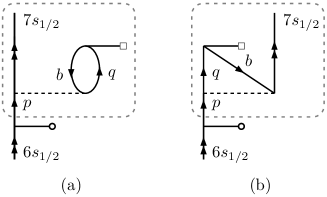
Figure 13: MBPT $E1_{\rm PNC}^{\rm NSD}$ diagrams used in the validation of the the singles PRCC amplitudes $S_{1}^{(1)}$.

VI.1 Single excitation operator $S_{1}^{(1)}$

To check the PRCC equation and angular momentum coupling in the calculations of $S_{1}^{(1)}$, consider the term ${S_{1}^{(1)}}^{\dagger}D$ in $E^{\rm NSD}_{\rm PNC}$. Two of the third order MBPT diagrams, which are equivalent to the ${S_{1}^{(1)}}^{\dagger}D$ at the first iteration of the PRCC equation are shown in Fig. 13. In the figure, the portion of the diagrams within the rectangle of dashed-line arises from the second order wave operator ${\Omega_{7s,1}^{(1)}}^{\dagger}$ define in Eq. (17). As for the solutions of linearized PRCC equations, the initial guess is the first order MBPT wave function $\Omega_{7s,1}^{(0)}$. Single excitation cluster amplitudes $\bm{\tau}$ are then calculated iteratively from Eq. (30). At the first iteration of the linearized PRCC equation, the diagram within the dashed rectangle in Fig. 13(a) is equal to the one valence version of the diagram in Fig. 4(c). And, the diagram Fig. 13(b) is the exchange counterpart. These MBPT diagrams are the dominant ones after the DF and other theories like the PRCC must be able to reproduce matching results.

Table 1: Validation of singles PRCC amplitudes. The values listed are in units of $iea_{0}\mu{{}^{\prime}}_{w}$. Numbers in the square bracket represent the power of 10.

Orbital ($p$,$q$)	MBPT	PRCC
$6p_{1/2}$	$3.80237[-15]$	$3.80237[-15]$
$7p_{1/2}$	$-4.42335[-16]$	$-4.42335[-16]$
$8p_{1/2}$	$1.08456[-16]$	$1.08456[-16]$
$9p_{1/2}$	$1.88997[-16]$	$1.88997[-16]$
$10p_{1/2}$	$8.66134[-17]$	$8.66134[-17]$
$11p_{1/2}$	$2.41491[-18]$	$2.41491[-18]$

For comparison, $E1_{\rm PNC}^{\rm NSD}$ contribution from the two diagrams in Fig. 4 from MBPT and results from the equivalent PRCC calculations are listed in Table. 1. The specific orbital wise contributions, for better comparison, of the dominant contributions are listed in the table. It is evident that there is excellent agreement between the MBPT and PRCC results.

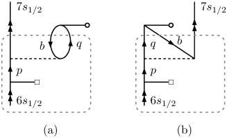
Figure 14: MBPT $E1_{\rm PNC}^{\rm NSD}$ diagrams used in the validation of the doubles PRCC amplitudes $S_{2}^{(1)}$.

VI.2 Double excitation operator $S_{2}^{(1)}$

Like in the case of $S_{1}^{(1)}$, consider two MBPT diagrams which are equivalent to the $S_{2}^{(1)}$ diagram after the first iteration and are shown in Fig. 14. In the figure, the portion of the diagrams within the rectangle in dashed-lines are equivalent to the $S_{2}^{(1)}$ diagram in Fig. 5(a) but adapted for one-valence systems. However, there is a major difference from the $S_{1}^{(1)}$. As $H_{\rm PNC}^{\rm NSD}$ is a single particle operator, the double excitation cluster operator at one order of $H_{\rm PNC}^{\rm NSD}$ is zero and the initial guess value is set to zero. To provide a wider test sample, for the double excitation the MBPT diagrams considered are equivalent to the term $DS_{2}^{(1)}$ in PRCC. Another variation is, the two diagrams considered in $S_{1}^{(1)}$ arise from topologically different diagrams, in the present case, the two diagrams in Fig. 14 arise from the same $S_{2}^{(1)}$ but different cluster amplitudes.

Table 2: Validation of doubles PRCC amplitudes. The values listed are in units of $iea_{0}\mu{{}^{\prime}}_{w}$. Numbers in the square bracket represent the power of 10.

Orbital ($p,q$)	MBPT	PRCC
$6p_{1/2}$	$6.53322[-17]$	$6.53322[-17]$
$7p_{1/2}$	$2.35102[-17]$	$2.35102[-17]$
$8p_{1/2}$	$3.20651[-16]$	$3.20651[-16]$
$9p_{1/2}$	$2.02539[-15]$	$2.02539[-15]$
$10p_{1/2}$	$8.67435[-16]$	$8.67435[-16]$
$11p_{1/2}$	$3.02443[-17]$	$3.02443[-17]$

The results from the MBPT and PRCC calculations are listed in Table. 2. Here too, the results from the two calculations are in excellent agreement. Perhaps, it must be mentioned that, the angular momentum factor calculations of the MBPT and PRCC diagrams are done in very different steps. Electronic part of the portion within the rectangle in dashed-line in Fig. 14 are evaluated to reduce to the representation of $S_{2}^{(1)}$ as discussed in Section. III.2. MBPT diagrams, on the other hand, may be evaluated without the need to associate with an effective operator of specific form.

VII Conclusions

The relativistic coupled-cluster method we have developed to incorporate a nuclear spin-dependent perturbation is an apt one to calculate nuclear spin-dependent parity non-conservation in atoms and ions. The representation of the cluster amplitude within the electronic sector as a tensor operator of rank one and coupling with the nuclear spin part at a later stage of property calculation leads to simplification of the calculations. Otherwise, the entire calculation must be done with hyperfine states, which involves complicated angular momentum couplings at all stages of the calculations. The proposed scheme, on the other hand, introduces the nuclear spin coupling is with a simplified effective operator in the electronic sector. The validity of the representation is explicitly tested and verified with selected diagrams. Although limited in number, the diagrams and terms selected in the sample test calculations are varied enough to account for complex as well as subtle issues related to the method. Based on the results presented, we conclude that the method works and in future publications we shall report results of sophisticated and large scale calculations using PRCC.

*

Appendix A Angular factors of PRCC equation

Here, we give the linearized PRCC equations of the closed-shell sector, Eqs. (30) and (34), after angular integration. The one-valence cluster amplitude equations can be obtained after suitable modifications.

A.1 Single excitation cluster operator

The angular reduction of each diagram is such that the free parts are reduced to the form in Fig. 3(a). The free part is common to all the diagrams and is avoided in the computational implementation. So, solutions of the PRCC equations are the cluster amplitudes in reduced matrix form. For $T_{1}^{(1)}$ and $S_{1}^{(1)}$, the rank of the operator, and hence the free part, is one. For convenience, the representation of $T_{2}^{(1)}$ is redefined as

$$\mathbf{T}^{(1)}_{2}=\sum_{abpq}\sum_{l_{1},l_{2}}\tau_{ab}^{pq}(l_{1},l_{2})\{\mathbf{C}_{l_{1}}(\hat{r}_{1})\mathbf{C}_{l_{2}}(\hat{r}_{2})\}^{1}.$$ (64)

Like the PRCC operators, we use $t^{p}_{a}$ and $t^{pq}_{ab}$ to represent the unperturbed single and double excitation amplitudes, respectively. The tensor operator structure of $T^{(0)}_{2}$ is

$$T^{(0)}_{2}=\sum_{abpq}\sum_{k}t_{ab}^{pq}(k)\mathbf{C}_{k}(\hat{r}_{1})\cdot\mathbf{C}_{k}(\hat{r}_{2}).$$ (65)

For the Slater integrals, the reduced matrix element is

$$X_{k}(abcd)=(-1)^{k}\langle\kappa_{a}|\!|\mathbf{C}^{k}|\!|\kappa_{c}\rangle\langle\kappa_{b}|\!|\mathbf{C}^{k}|\!|\kappa_{d}\rangle R_{k}(abcd),$$ (66)

where, $R_{k}(abcd)$ is the radial part of the Slater integral. With these definitions, the Eq. (30) is written in terms of reduced matrix elements and appropriate angular factors.

$$(\epsilon_{a}- \epsilon_{p} )\bm{\tau}^{p}_{a}=\bm{h}_{pa}+\sum_{q}\frac{\delta{(j_{a},j_{q}})}{\sqrt{(2j_{a}+1)}}\bm{h}_{pq}t^{q}_{a}-\sum_{b}\frac{\delta{(j_{b},j_{p}})}{\sqrt{(2j_{b}+1)}}\bm{h}_{ba}t^{p}_{b}+\sum_{bqk_{2}}\bm{h}_{bq}\left[\frac{\delta{(k_{1},k_{2}})}{\sqrt{(2k_{1}+1)}}(-1)^{j_{q}-j_{b}+k_{1}}t^{qp}_{ba}(k_{2})\right.$$ (87)

$$-(-1)^{j_{b}+j_{q}+k_{1}}\left\{\begin{array}[]{ccc}j_{b}&j_{q}&k_{1}\\ j_{a}&j_{p}&k_{2}\end{array}\right\}t^{qp}_{ab}(k_{2})\Bigg{]}+\sum_{bqk_{2}}\bm{\tau}^{q}_{b}\Bigg{[}\frac{\delta{(k_{1},k_{2}})}{\sqrt{(2k_{1}+1)}}(-1)^{j_{q}-j_{b}+k_{1}}X_{k_{2}}(bpqa)$$

$$-(-1)^{j_{b}+j_{q}+k_{1}}\left\{\begin{array}[]{ccc}j_{a}&j_{b}&k_{2}\\ j_{q}&j_{p}&k_{1}\end{array}\right\}X_{k_{2}}(bpaq)\Bigg{]}+\sum_{bqrk_{2}}\sum_{l_{1}l_{2}}\bm{\tau}^{qr}_{ba}(l_{1},l_{2})\Bigg{[}\frac{\delta{(k_{2},l_{2}})}{\sqrt{(2k_{2}+1)}}(-1)^{j_{q}-j_{b}+j_{a}+j_{p}+l_{1}}$$

$$\times\;\left\{\begin{array}[]{ccc}j_{r}&j_{a}&l_{1}\\ k_{1}&k_{2}&j_{p}\end{array}\right\}X_{k_{2}}(bpqr)-(-1)^{j_{a}+j_{p}+j_{b}+j_{q}+l_{1}}\left\{\begin{array}[]{ccc}j_{b}&k_{2}&j_{r}\\ j_{p}&l_{2}&j_{q}\end{array}\right\}\left\{\begin{array}[]{ccc}j_{r}&j_{a}&l_{1}\\ k_{1}&l_{2}&j_{p}\end{array}\right\}X_{k_{2}}(bprq)\Bigg{]}$$

$$-\sum_{bcqk_{2}}\sum_{l_{1}l_{2}}X_{k_{2}}(bcqa)\Bigg{[}\frac{\delta{(k_{2},l_{2}})}{\sqrt{(2k_{2}+1)}}(-1)^{j_{a}-j_{b}+j_{p}+j_{q}+k_{1}+k_{2}}\left\{\begin{array}[]{ccc}j_{p}&l_{1}&j_{c}\\ k_{2}&j_{a}&k_{1}\end{array}\right\}\bm{\tau}^{qp}_{bc}(l_{1},l_{2})$$

$$-(-1)^{j_{q}+j_{c}+j_{a}+j_{p}+k_{1}+l_{2}}\left\{\begin{array}[]{ccc}k_{2}&j_{a}&j_{c}\\ l_{2}&j_{q}&j_{b}\end{array}\right\}\left\{\begin{array}[]{ccc}j_{b}&j_{p}&l_{1}\\ k_{1}&l_{2}&j_{a}\end{array}\right\}\bm{\tau}^{qp}_{cb}(l_{1},l_{2})\Bigg{]}.$$

A.2 Double excitation cluster operator

For the double excitation PRCC operator $T_{2}^{(1)}$, the common free part of the angular factors in Eq. (34) is as shown in Fig. 3(b). In the angular factors, the multipoles $k_{1}$, $k_{2}$, $l_{1}$ and $l_{2}$ have the same interpretations as in the singles. Multipoles $l_{3}$ and $l_{4}$ are, however, arise from coupling $(j_{a},j_{p})$ and $(j_{b},j_{q})$, respectively. The double excitation cluster equation obtained from the projection on $\langle\Phi_{ab}^{pq}|$ along with appropriate angular factors is

$$(\epsilon_{a}+ \epsilon_{b} -\epsilon_{p}-\epsilon_{q})\bm{\tau}^{pq}_{ab}(l_{1},l_{2})=\Bigg{[}\sum_{r}(2l_{1}+1)(-1)^{j_{a}+j_{p}+k_{1}+l_{2}}\left\{\begin{array}[]{ccc}k_{1}&j_{p}&j_{r}\\ j_{a}&l_{2}&l_{1}\end{array}\right\}\bm{h}_{pr}t^{rq}_{ab}(l_{2})-\sum_{c}(2l_{1}+1)$$ (129)

$$\times\;(-1)^{j_{a}+j_{p}+l_{1}}\left\{\begin{array}[]{ccc}k_{1}&j_{a}&j_{c}\\ j_{p}&l_{2}&l_{1}\end{array}\right\}\bm{h}_{ca}t^{pq}_{cb}(l_{2})+\sum_{r}(2l_{1}+1)(-1)^{j_{a}+j_{p}+l_{1}}\left\{\begin{array}[]{ccc}l_{2}&j_{p}&j_{r}\\ j_{a}&k_{1}&l_{1}\end{array}\right\}X_{l_{2}}(pqrb)\bm{\tau}^{r}_{a}$$

$$-\sum_{c}(2l_{1}+1)(-1)^{j_{a}+j_{p}+k_{1}+l_{2}}\left\{\begin{array}[]{ccc}l_{2}&j_{a}&j_{c}\\ j_{p}&k_{1}&l_{1}\end{array}\right\}X_{l_{2}}(cqab)\bm{\tau}^{p}_{c}+\sum_{rc}\frac{1}{(2l_{1}+1)}(-1)^{j_{r}-j_{c}+l_{1}}$$

$$\times X_{k_{2}}(pcar)\bm{\tau}^{rq}_{cb}(l_{1},l_{2})-\sum_{rc}\sum_{l_{3}l_{4}}(2l_{2}+1)(-1)^{j_{c}-j_{q}+k_{1}+l_{3}}\left\{\begin{array}[]{ccc}j_{r}&l_{3}&j_{b}\\ j_{c}&l_{4}&j_{q}\\ l_{1}&k_{1}&l_{2}\end{array}\right\}X_{l_{1}}(pcar)\bm{\tau}^{rq}_{bc}(l_{3},l_{4})$$

$$-\sum_{rck_{2}}\sum_{l_{3}l_{4}}(2l_{1}+1)(2l_{2}+1)(-1)^{j_{a}+j_{p}+j_{b}+j_{q}+k_{1}}\left\{\begin{array}[]{ccc}k_{2}&j_{p}&j_{r}\\ j_{a}&l_{3}&l_{1}\end{array}\right\}\left\{\begin{array}[]{ccc}l_{2}&l_{1}&k_{1}\\ l_{3}&l_{4}&k_{2}\end{array}\right\}\left\{\begin{array}[]{ccc}k_{2}&j_{c}&j_{b}\\ j_{q}&l_{2}&l_{4}\end{array}\right\}X_{k_{2}}(pcrb)$$

$$\times\bm{\tau}^{rq}_{ac}(l_{3},l_{4})-\sum_{rck_{2}}(-1)^{j_{c}+j_{r}+l_{3}}\left\{\begin{array}[]{ccc}j_{a}&j_{c}&k_{2}\\ j_{r}&j_{p}&l_{1}\end{array}\right\}X_{k_{2}}(cpar)\bm{\tau}^{rq}_{cb}(l_{1},l_{2}),\Bigg{]}+\Bigg{[}\begin{array}[]{c}p\leftrightarrow q\\ a\leftrightarrow b\end{array}\Bigg{]}$$

$$+\sum_{rsk_{2}}\sum_{l_{3}l_{4}}(2l_{1}+1)(2l_{2}+1)(-1)^{j_{a}+j_{p}+j_{b}+j_{q}+k_{1}+k_{2}+l_{4}+l_{2}}\left\{\begin{array}[]{ccc}k_{2}&j_{p}&j_{r}\\ j_{a}&l_{3}&l_{1}\end{array}\right\}\left\{\begin{array}[]{ccc}l_{1}&l_{3}&k_{2}\\ l_{4}&l_{2}&k_{1}\end{array}\right\}\left\{\begin{array}[]{ccc}k_{2}&j_{s}&j_{q}\\ j_{b}&l_{2}&l_{4}\end{array}\right\}$$

$$\times X_{k_{2}}(pqrs)\bm{\tau}^{rs}_{ab}(l_{3},l_{4})+\sum_{cdk_{2}}\sum_{l_{3}l_{4}}(2l_{1}+1)(2l_{2}+1)(-1)^{j_{a}+j_{p}+j_{b}+j_{q}+k_{1}+k_{2}+l_{3}+l_{1}}\left\{\begin{array}[]{ccc}k_{2}&j_{a}&j_{c}\\ j_{p}&l_{3}&l_{1}\end{array}\right\}$$

$$\times\left\{\begin{array}[]{ccc}l_{2}&l_{1}&k_{1}\\ l_{3}&l_{4}&k_{2}\end{array}\right\}\left\{\begin{array}[]{ccc}k_{2}&j_{d}&j_{b}\\ j_{q}&l_{2}&l_{4}\end{array}\right\}X_{k_{2}}(cdab)\bm{\tau}^{pq}_{cd}(l_{3},l_{4}).$$

References

- (1) Y. Zel’dovich, JETP 6, 1184 (1958).
- (2) C. S. Wood, et al. Science 275, 1759 (1997).
- (3) N. Fortson, Phys. Rev. Lett. 70, 2383 (1993).
- (4) K. Tsigutkin, D. Dounas-Frazer, A. Family, J. E. Stalnaker, V. V. Yashchuk, and D. Budker, Phys. Rev. Lett. 103, 071601 (2009); Phys. Rev. A 81, 032114 (2010).
- (5) B. K. Sahoo, P. Mandal and M. Mukherjee, Phys. Rev. A 83 , 030502 (2011).
- (6) V. A. Dzuba and V. V. Flambaum, Phys. Rev. A 83, 042514 (2011).
- (7) V. A. Dzuba, V. V. Flambaum, and M. G. Kozlov, Phys. Rev. A 54, 3948 (1996).
- (8) S. G. Porsev, M. G. Kozlov, and Yu. G. Rakhlina, Hyperfine Interact. 127, 395 (2000).
- (9) V. A. Dzuba, V. V. Flambaum, arXiv:1104.0086.
- (10) K. P. Geetha, A. D. Singh, B. P. Das, and C. S. Unnikrishnan, Phys. Rev. A 58, R16 (1998).
- (11) A. D. Singh and B. P. Das, J. Phys. B 32, 4905 (1999).
- (12) B. K. Mani and D. Angom, arXiv:1104.3473v1.
- (13) F. Coester, Nucl. Phys. 7, 421 (1958).
- (14) F. Coester and H. Kümmel, Nucl. Phys. 17, 477 (1960).
- (15) R. Pal, M. S. Safronova, W. R. Johnson, A. Derevianko, and S. G. Porsev, Phys. Rev. A 75, 042515 (2007).
- (16) B. K. Sahoo, L. W. Wansbeek, K. Jungmann, and R. G. E. Timmermans, Phys. Rev. A 79, 052512 (2009).
- (17) H. S. Nataraj, B. K. Sahoo, B. P. Das, and D. Mukherjee, Phys. Rev. Lett. 101, 033002 (2008).
- (18) K. V. P. Latha, D. Angom, B. P. Das, and D. Mukherjee, Phys. Rev. Lett. 103, 083001 (2009).
- (19) C. Thierfelder and P. Schwerdtfeger, Phys. Rev. A 79, 032512 (2009).
- (20) B. K. Sahoo, B. P. Das, and D. Mukherjee, Phys. Rev. A 79, 052511 (2009).
- (21) L. W. Wansbeek, B. K. Sahoo, R. G. E. Timmermans, K. Jungmann, B. P. Das, and D. Mukherjee, Phys. Rev. A 78, 050501(R) (2008).
- (22) R. Pal, D. Jiang, M. S. Safronova, and U. I. Safronova, Phys. Rev. A 79, 062505 (2009).
- (23) S. G. Porsev, K. Beloy, and A. Derevianko, Phys. Rev. D 82, 036008 (2010).
- (24) B. K. Mani, K. V. P. Latha, and D. Angom, Phys. Rev. A 80, 062505 (2009).
- (25) B. K. Mani and D. Angom, Phys. Rev. A 81, 042514 (2010).
- (26) B. K. Sahoo and B. P. Das, Phys. Rev. A 77, 062516 (2008).
- (27) K. V. P. Latha, D. Angom, R. K. Chaudhari, B. P. Das and D. Mukherjee, J. Phys. B. 41, 035005 (2008).
- (28) I. Lindgren and J. Morrison, Atomic Many-Body Theory, edited by G. Ecker, P. Lambropoulos, and H. Walther (Springer-Verlag, 1985).
- (29) S. A. Blundell, W. R. Johnson, Z. W. Liu and J. Sapirstein, Phys. Rev. A 39, 3768 (1989).
- (30) S. A. Blundell, W. R. Johnson, Z. W. Liu and J. Sapirstein, Phys. Rev. A 40, 2233 (1989).
- (31) B. K. Mani and D. Angom, Phys. Rev. A 83, 012501 (2011).