Observation of Evolutionary Velocity Field in Matching Pennies Game

Abstract

Matching pennies game is the simplest game in game theory. In data from laboratory experimental economics, with the metric for an instantaneous velocity measurement, we report the first observation of the evolutionary velocity field in the population strategy state space of the game.

Background: In evolutionary game theory (EGT), an evolutionary dynamic equation describes the velocity field. A velocity field quantifies the direction and the magnitude of the populations’ strategy state change ($\triangle x$) in a unit of time ($\triangle t$) at each given state $x$ in the populations’ strategy state space $\mathbb{X}$ Traulsen and Hauert (2010); Weibull (1997); Bowles (2004); Sigmund (2010).

Laboratory experimental economics removes EGT from its abstract setting and links the theory to observed behavior Samuelson (2002). The observed populations behavior in the experiments are systematic, replicable, and roughly consistent with the dynamical systems approach Crawford (1991); Binmore et al. (1993); Van Huyck et al. (1995); Binmore et al. (2001); Battalio et al. (2001); Cason et al. (2005). The evolutionary velocity field has never before been obtained empirically. In this letter, we will use a laboratory matching pennies game (MPG) to experimentally obtain the the evolutionary velocity field.

Space, State and Time: In EGT analogy Sigmund (2010), without loss of generality, we use a two-population MPG as an example. In the first population $X$, the strategy set is $\{X_{1}$,$X_{2}\}$ for each agent; similarly, in the second population $Y$, it is $\{Y_{1}$,$Y_{2}\}$. The payoff matrix is in shown Table 1 . If there are 4 agents in each population, an observable instantaneous populations strategy state should be $x$:=$(p,q)\in\mathbb{X}$. $\mathbb{X}$ is the populations strategy state space and $\mathbb{X}$=$\{0,\frac{1}{4},\frac{2}{4},\frac{3}{4},1\}\bigotimes\{0,\frac{1}{4},\frac{2}{4},\frac{3}{4},1\}$, and $p$ ($q$) is the density of $X_{1}$ ($Y_{1}$) in $X$ ($Y$). Figure 1 is an illustration, in which the square $5\times 5$ lattice (gray dots) is the space $\mathbb{X}$ and $x_{A}$=($\frac{1}{4},\frac{3}{4}$) is a state.

In experimental economics, the time $t$ is the label along the repeated rounds in a session. At each round $t$, there is one observation of $x_{t}$ in $\mathbb{X}$. Therefore, the smallest tick $\triangle t$ is $1$ and is the time interval between two successive rounds.

Table 1: Payoff matrix of the MPG

	$Y_{1}$	$Y_{2}$
$~{}X_{1}~{}$	$~{}5~{}~{}~{}~{}~{}$	$~{}0~{}~{}~{}~{}~{}$
	$~{}~{}~{}~{}~{}0~{}$	$~{}~{}~{}~{}~{}5~{}$
$~{}X_{2}~{}$	$~{}0~{}~{}~{}~{}~{}$	$~{}5~{}~{}~{}~{}~{}$
	$~{}~{}~{}~{}~{}5~{}$	$~{}~{}~{}~{}~{}0~{}$

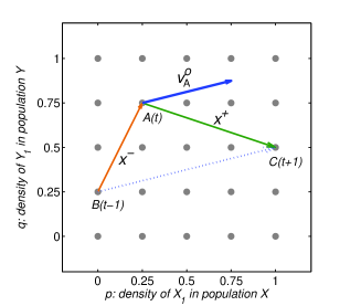
Figure 1: Schematic diagram for an observation of an instantaneous velocity $v^{o}_{pq}$. The $5\times 5$ Lattice (in gray dots) is the population strategy state space $\mathbb{X}$ of the two populations MPG. $x_{A}$ is one of the states in $\mathbb{X}$ and $x_{A}$=$(0.25,0.75)$. Suppose that, during a microscope process $\mathbb{P}$ including both a forward change ($x^{+}$) and a backward chang ($x^{-}$), the observed state at $t$ is $x_{A}$, and at ($t-1$) is $x_{B}$ and at ($t+1$) is $x_{C}$, by Eq. (1), $v^{o}_{A}$=$(x_{C}-x_{B})/2$ (arrow in blue) is an instantaneous velocity at $x_{A}$.

Metric for Velocity: Figure 1 shows a microscopic process $\mathbb{P}$ from which one observation of an instantaneous velocity, $\upsilon^{o}_{pq}$, can be defined Xu and Wang (2011). From $t$ to $t$+$1$, the forward change at a given state $(p,q)$ is described as $x^{+}$=$x_{t+1}-x_{t}$. From $t$-$1$ to $t$, the backward change is $x^{-}$=$x_{t}-x_{t-1}.$ Hence, at a given state $(p,q)$, we define, $\upsilon^{o}_{pq}$, as

$$\upsilon^{o}_{pq}:=\left(x^{+}+x^{-}\right)/(2\triangle t).$$ (1)

Practically, in experimental economics, $\triangle t$=1. In Eq.(1), $\upsilon^{o}_{pq}$ satisfies two requirements for the measurement of instantaneous velocity (1) instantaneous: time interval is practically the smallest; (2) time odd: it is time reversal asymmetric . Then, the mean velocity vector at the $(p,q)$ can be computed as

$$\overline{\upsilon}_{pq}=\frac{1}{\Omega_{pq}}\sum_{o}\upsilon^{o}_{pq},$$ (2)

where $\Omega_{pq}$ is the total observation of the state $(p,q)$ and the summation is carried over all of the rounds whenever the observed state is $(p,q)$. A practical numeric example for calculation of a $\overline{\upsilon}_{pq}$ is shown in the S2 in electronic supplementary materials.

Experiment: This experiment uses the traditional experimental setting for social evolution Crawford (1991); Binmore et al. (1993); Van Huyck et al. (1995); Binmore et al. (2001); Battalio et al. (2001); Cason et al. (2005); Selten and Chmura (2008). We employed the MPG among two populations with the payoff matrix in Table 1. Each population includes 4 subjects. There are 12 independent sessions and each session includes 300 rounds repeated with random matching protocol. For more details, see S1 in the electronic supplementary materials.

Results: Figure 2 shows the main results from our experimental data for the MPG. The mean observation of density is $x^{*}$=$(0.510,0.490)$. For each state, Figure 2 shows the total number of observation $\Omega_{pq}$ and the mean velocity vector $\overline{\upsilon}_{pq}$. Globally, a significant cyclic velocity field pattern is observed.

For state $(p,q)$, the normal vector is defined as $r_{pq}$:=$x_{pq}-x^{*}$. Our results show a statistically significant positive correlation between $|\overline{\upsilon}_{pq}|$ and $|r_{pq}|$ ($p$=0.000); The angle from $\overline{\upsilon}_{pq}$ to $r_{pq}$ is a right angle ($\pm 7\%$) .

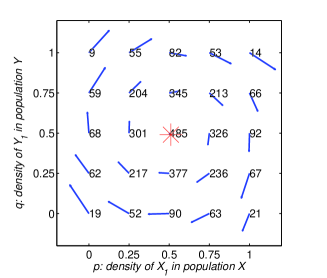
Figure 2: Obtained evolutionary velocity field in laboratory MPG. The red star ($\ast$) indicates the mean observation of density. The numeric label indicates the observed occupation $\Omega_{pq}$ of each state. The blue arrow from each state indicates the direction and the magnitude of mean velocity $\overline{\upsilon}_{pq}$. The plotting ratio is $1:1$.

Summary: In our data of MPG, statistically, the larger the magnitude of the normal vector, the faster the evolution should be. Meanwhile, the direction of the evolution is perpendicular to the normal vector. In the full population strategy state space, the evolutionary velocity field pattern is cyclic and clockwise.

The existence of the velocity pattern is not observed only in our data. Using the same experimetrics as above and the data from ref. Selten and Chmura (2008) and ref. Binmore et al. (2001), which contains 19 different payoff matrix treatments of 2$\times$2 games of laboratory experimental economics, results of the significant cyclic velocity fields are als observed. For more details see S3 in the electronic supplementary materials.

The matching pennies game is the simplest model in game theory Von Neumann and Morgenstern (1944) and the evolution dynamical pattern can be modeled theoretically Weibull (1997); Sandholm (2011). In this letter, we report the first empirical observation of the evolutionary velocity field.

Acknowledgment: Thanks to B. O’Neill, K. Binmore, Y. Chen, R. Selten, S. Sunder, T. N. Cason, A. Roth, S. J. Goerg, H. Wu, Y. Jia, Z. Dong, J. Wooders and Q. Cheng for the valuable comments and/or providing data. Comments from ESA-PA 2011, ESA-EU 2011 conference and EEF Workshop in Xiamen University 2010 were helpful.

References

- Traulsen and Hauert (2010) A. Traulsen and C. Hauert, Stochastic Evolutionary Game Dynamics, Reviews of Nonlinear Dynamics and Complexity (Wiley-VCH Verlag GmbH & Co. KGaA, 2010).
- Weibull (1997) J. Weibull, Evolutionary game theory (The MIT press, 1997).
- Bowles (2004) S. Bowles, Microeconomics: behavior, institutions, and evolution (Princeton University Press, 2004).
- Sigmund (2010) K. Sigmund, The calculus of selfishness (Princeton Univ Pr, 2010).
- Samuelson (2002) L. Samuelson, The Journal of Economic Perspectives 16, 47 (2002).
- Crawford (1991) V. Crawford, Games and Economic Behavior 3, 25 (1991).
- Binmore et al. (1993) K. Binmore, J. Swierzbinski, S. Hsu, and C. Proulx, International Journal of Game Theory 22, 381 (1993).
- Van Huyck et al. (1995) J. Van Huyck, R. Battalio, S. Mathur, P. Van Huyck, and A. Ortmann, International Journal of Game Theory 24, 187 (1995).
- Binmore et al. (2001) K. Binmore, J. Swierzbinski, and C. Proulx, The Economic Journal 111, 445 (2001).
- Battalio et al. (2001) R. Battalio, L. Samuelson, and J. Van Huyck, Econometrica 69, 749 (2001).
- Cason et al. (2005) T. Cason, D. Friedman, and F. Wagener, Journal of Economic Dynamics and Control 29, 801 (2005), ISSN 0165-1889.
- Xu and Wang (2011) B. Xu and Z. Wang, Evolutionary Dynamical Pattern of ”Coyness and Philandering”: Evidence from Experimental Economics, vol. 3 (p1313-1326, NECSI Knowledge Press, ISBN 978-0-9656328-4-3., 2011).
- Selten and Chmura (2008) R. Selten and T. Chmura, The American Economic Review 98, 938 (2008).
- Von Neumann and Morgenstern (1944) J. Von Neumann and O. Morgenstern, Theory of games and economic behavior. (Princeton University Press, 1944).
- Sandholm (2011) W. Sandholm, Population games and evolutionary dynamics (MIT press Cambridge, MA:, 2011).
- Meijer and Bauer (2004) P. Meijer and E. Bauer, Group theory: the application to quantum mechanics (Dover Pubns, 2004).