Recursive Bias Estimation for multivariate regression smoothers

Abstract

This paper presents a practical and simple fully nonparametric multivariate smoothing procedure that adapts to the underlying smoothness of the true regression function. Our estimator is easily computed by successive application of existing base smoothers (without the need of selecting an optimal smoothing parameter), such as thin-plate spline or kernel smoothers. The resulting smoother has better out of sample predictive capabilities than the underlying base smoother, or competing structurally constrained models (GAM) for small dimension ($3\leq d\leq 7$) and moderate sample size $n\leq 800$. Moreover our estimator is still useful when $d>10$ and to our knowledge, no other adaptive fully nonparametric regression estimator is available without constrained assumption such as additivity for example. On a real example, the Boston Housing Data, our method reduces the out of sample prediction error by 20%. An R package ibr, available at CRAN, implements the proposed multivariate nonparametric method in R.

, and

1 Introduction

Regression is a fundamental data analysis tool for uncovering functional relationships between pairs of observations $(X_{i},Y_{i}),i=1,\ldots,n$. The traditional approach specifies a parametric family of regression functions to describe the conditional expectation of the response variable $Y$ given the independent multivariate variables $X\in\mathbb{R}^{d}$, and estimates the free parameters by minimizing the squared error between the predicted values and the data. An alternative approach is to assume that the regression function varies smoothly in the independent variable $x$ and then estimate locally the conditional expectation $m(x)={\mathbb{E}}[Y|X=x]$. This results in nonparametric regression estimators. We refer the interested reader to Eubank (1999), Fan and Gijbels (1996) and Simonoff (1996) for a more in depth treatment of various classical regression smoothers. The vector of predicted values $\widehat{Y}_{i}$ at the observed covariates $X_{i}$ from a nonparametric regression is called a regression smoother, or simply a smoother, because the predicted values $\widehat{Y}_{i}$ are less variable than the original observations $Y_{i}$. Operationally, linear smoothers can be written as

$$\widehat{m}=SY,$$

where $S$ is a $n\times n$ smoothing matrix. Smoothing matrices $S$ (or $S_{\lambda}$) typically depend on a tuning parameter, which we denote by $\lambda$, that governs the tradeoff between the smoothness of the estimate and the goodness-of-fit of the smoother to the data, by controlling the effective size of the local neighborhood of the explanatory variable over which the responses are averaged. We parameterize the smoothing matrix such that large values of $\lambda$ will produce very smooth curves while small $\lambda$ will produce a more wiggly curve that wants to interpolate the data. For example, the tuning parameter $\lambda$ is the bandwidth for kernel smoother, the span size for running-mean smoother, and the scalar that governs the smoothness penalty term for thin plate splines (TPS).

It is well known that given $n$ uniformly distributed points in the unit cube $[-1,1]^{d}$, the expected number of points that are covered by a ball centered at the origin with radius $\varepsilon<1$, scales as $n\varepsilon^{d}$. This is to say that covariates in high dimensions are typically sparse. This phenomenon is sometimes called the curse of dimensionality. As a consequence, nonparametric smoothers must average over larger neighborhoods, which in turn produces more heavily biased smoothers. Optimally selecting the smoothing parameter does not alleviate this problem. Indeed, when the regression function $m$ mapping ${\mathbb{R}}^{d}$ to ${\mathbb{R}}$ belongs to some finite smoothness functional classes (Hölder, Sobolev, Besov) the optimal mean squared error rate of convergence is $n^{-2\nu/(2\nu+d)}$ where $\nu$ is the smoothing index (see for example Tsybakov, 2009). Common wisdom suggest avoiding general nonparametric smoothing in moderate dimensions (say $d>5$) and focus instead on fitting structurally constrained regression models, such as additive (Hastie and Tibshirani, 1995; Linton and Nielsen, 1995; Hengartner and Sperlich, 2005) and projection pursuit models (Friedman and Stuetzle, 1981). The popularity of additive models stems in part from the interpretability of the individual estimated additive components, and from the fact that the estimated regression function converges to the best additive approximation of the true regression function at the optimal univariate mean squared error rate of $n^{-2\nu/(2\nu+1)}$. While additive models do not estimate the true underlying regression function, one hopes for the approximation error to be small enough so that for moderate sample sizes, the prediction mean square error of the additive model is less than the prediction error of a fully nonparametric regression model.

The impact of the curse of dimensionality is lessened for very smooth regression functions. For regression functions with $\nu=2d$ continuous derivatives, the optimal rate is $n^{-4/5}$, a value recognized as the optimal mean squared error of estimates for twice differentiable univariate regression functions. The difficulty is that in practice, the smoothness of the regression function is typically unknown. Nevertheless, there are large potential gains (in terms of rates of convergence) if one considers multivariate smoothers that adapt to the smoothness of the regression function. Since the pioneer work of Lepski (1991), adaptive nonparametric estimation became a major topic in mathematical statistics (see for example Gyorfi et al. 2002 or Tsybakov 2009). Adaptive nonparametric estimator can be achieve either by direct estimation (see Lepski’s method and related papers) or by aggregation of different procedures (see Yang, 2000). This paper presents a practical and simple nonparametric multivariate smoothing procedure that adapts to the underlying smoothness of the true regression function. Our estimator is easily computed by successive application of existing smoothers, such as Thin Plate Spline or kernel smoother. Thanks to adaptivity (proven for TPS smoother), our estimator behaves nicely in small dimension ($3\leq d\leq 7$) with moderate sample size $n\leq 800$ and remains useful when $d>10$.

Section 2 introduces our procedure and motivates it as repeated corrections to the bias of a smoother, where at each step, the bias is estimated by smoothing the residuals. We use the Generalized Cross-Validation (GCV) criteria to stop our iterative procedure when the prediction error of our estimate is nearly minimized. The idea of estimating the bias from residuals to correct a pilot estimator of a regression function goes back to the concept of twicing introduced by Tukey (1977) to estimate bias of misspecified multivariate regression models. Numerous authors have shown the benefits of various bias reduction techniques in nonparametric regression, including He and Huang (2009); Choi et al. (2000); Choi and Hall (1998); Hengartner et al. (2010); Hirukawa (2010).

The idea of iterative debiasing regression smoothers is already present in Breiman (1999) in the context of the bagging algorithm. More recently, the interpretation of the $L_{2}$-boosting algorithm as an iterative bias correction scheme was alluded to in Ridgeway (2000)’s discussion of Friedman et al. (2000) paper on the statistical interpretation of boosting. Bühlmann and Yu (2003) present the statistical properties of the $L_{2}$-boosted univariate smoothing splines and proposed an additive procedure to deal with multivariate data. Di Marzio and Taylor (2008) describes the behavior of univariate kernel smoothers after a single bias-correction iteration.

Section 3 applies the iterative bias reduction procedure to multivariate Thin Plate Spline smoothers. TPS smoothers have attractive theoretical properties that facilitate our proofs of the adaptation to the unknown smoothness of our procedure. However, implementation of the TPS is limited by the need of the sample size to be larger than size of its parametric component. The latter grows exponentially with the dimension of the covariates $d$. For practical considerations, we consider, in Section 4, the iterative bias reduction procedure using kernel smoothers that can be applied more generally than TPS. We discuss the use of different kernels since the choice of the kernel is important for the iterative bias reduction procedure.

The simulation results presented in Section 5 show that for moderate dimensions of the covariates (eg. $3\leq d\leq 7$), and sample sizes ranging from $n=50$ to $n=800$, our iterated smoother has significantly smaller prediction error than the base smoother with using an “optimal smoothing” parameter. We end this section with the prediction of the classical Boston housing data set ($n=506$ and $d=13$). The interested reader can download an R implementation of our procedure with optimized computations for moderate sample size (Cornillon et al., 2010).

Finally, the proofs are gathered in the Appendix.

2 Iterative bias reduction

This section presents the general iterative bias reduction framework for linear regression smoothers and shows that the resulting smoother, when combined with GCV, adapts to the underlying smoothness of the regression function. The advantage of our smoother is its simplicity: we only need to repeatedly smooth residuals using existing multivariate smoothers. The cost of adaptation is an increase in computational complexity.

2.1 Preliminaries

Suppose that the pairs $(X_{i},Y_{i})\in{\mathbb{R}}^{d}\times{\mathbb{R}}$ are related through the regression model

$$Y_{i} = m(X_{i})+\varepsilon_{i},\quad i=1,\ldots,n,$$ (1)

where $m(\cdot)$ is an unknown smooth function, and the disturbances $\varepsilon_{i}$ are independent mean zero and variance $\sigma^{2}$ random variables that are independent of all the covariates $(X_{1},\ldots,X_{n})$. It is helpful to rewrite Equation (1) in vector form by setting $Y=(Y_{1},\ldots,Y_{n})^{\prime}$, $m=(m(X_{1}),\ldots,m(X_{n}))^{\prime}$ and $\varepsilon=(\varepsilon_{1},\ldots,\varepsilon_{n})^{\prime}$, to get

$$Y = m+\varepsilon.$$ (2)

Linear smoothers can be written as

$$\widehat{m}=S_{\lambda}Y,$$ (3)

where $S_{\lambda}$ is an $n\times n$ smoothing matrix and $\widehat{m}=(\widehat{Y}_{1},\ldots,\widehat{Y}_{n})^{\prime}$, denotes the vector of fitted values. From now on, we denote the smoothing matrix by $S$. Let $I$ be the $n\times n$ identity matrix. The bias of the linear smoother (3), conditionally on the observed values of the covariates $X_{1}^{n}=(X_{1},\ldots,X_{n})$, is

$$\mathbb{E}[\widehat{m}|X_{1}^{n}]-m = (S-I)m=-\mathbb{E}[(I-S)Y|X_{1}^{n}].$$ (4)

2.2 Bias reduction of linear smoothers

Expression (4) for the bias suggests that it can be estimated by smoothing the negative residuals $-R=-(Y-\widehat{m})=-(I-S)Y$. An alternative approach is to estimate the bias by plugging in an estimator for the regression function $m$ into the expression (4). The resulting estimators are different except if we consider using the same smoother for estimating the bias and for estimating the initial smoother. From now on, we consider using the same smoother. The initial estimator is given by

$$\hat{m}_{1} = SY:=S_{1}Y.$$

Smoothing the residuals

$$\hat{b}_{1}:=-SR_{1}=-S(I-S_{1})Y$$

estimates the bias. Correcting the initial smoother $\widehat{m}_{1}$ by subtracting $\hat{b}_{1}$ yields a bias corrected smoother

$$\widehat{m}_{2} = S_{1}Y-\hat{b}_{1}$$

$$= S_{1}Y+S(I-S_{1})Y:=S_{2}Y.$$

Since $\hat{m}_{2}$ is itself a linear smoother, it is possible to correct its bias as well. Repeating the bias reduction step $k-1$ times produces the linear smoother at iteration $k$:

$$\widehat{m}_{k} = S_{k-1}Y+S(I-S_{k-1})Y:=S_{k-1}Y-\hat{b}_{k-1}:=S_{k}Y$$

The resulting $k^{th}$ iterated bias corrected smoother becomes

$$\hat{m}_{k}=[I-(I-S)^{k}]Y:=S_{k}Y.$$ (5)

In the univariate case, smoothers of the form (5) arise from the $L_{2}$-boosting algorithm when setting the convergence factor $\mu_{k}$ of that algorithm to one. Thus we can interpret the $L_{2}$-boosting algorithm as an iterative bias reduction procedure. From that interpretation, it follows that the $L_{2}$-boosting of projection smoothers, as is the case for polynomial regression, bin smoothers and regression splines, is ineffective since the estimated bias

$$\hat{b}=S(I-S)Y=0.$$

2.3 Predictive smoothers

Our smoothers predict the conditional expectation of responses only at the design points. It is useful to extend regression smoothers to enable predictions at arbitrary locations $x\in{\mathbb{R}}^{d}$ of the covariates. Such an extension allows us to assess and compare the quality of various smoothers by how well the smoother predicts new observations. To this end, write the prediction of the linear smoother $S$ at an arbitrary location $x$ as

$$\hat{m}(x)=S(x)^{\prime}Y,$$

where $S(x)$ is a vector of size $n$ whose entries are the weights for predicting $m(x)$. The vector $S(x)$ is readily computed for many of the smoothers used in practice. Next, writing the iterative bias corrected smoother $\widehat{m}_{k}$ as

$$\widehat{m}_{k} = \widehat{m}_{1}-\widehat{b}_{1}+\dots-\widehat{b}_{k-1}$$

$$= S[I+(I-S)+(I-S)^{2}+\dots+(I-S)^{k-1}]Y$$

$$= S\widehat{\beta}_{k},$$

it follows that we can predict $m(x)$ by

$$\widehat{m}_{k}(x)=S(x)^{\prime}\widehat{\beta}_{k}.$$ (6)

2.4 Properties of iterative bias corrected smoothers

The squared bias and variance of the $k^{th}$ iterated bias corrected smoother $\widehat{m}_{k}$ (5) are

$$\left(\mathbb{E}[\hat{m}_{k}|X_{1}^{n}]-m\right)^{2} = m^{\prime}\left((I-S)^{k}\right)^{\prime}(I-S)^{k}m$$

$$\mathrm{var}(\hat{m}_{k}|X_{1}^{n}) = \sigma^{2}(I-(I-S)^{k})\left((I-(I-S)^{k})\right)^{\prime},$$

This shows that the qualitative behavior of the sequence of iterative bias corrected smoothers $\widehat{m}_{k}$ can be related to the spectrum of $I-S$. The next proposition collects the various results for sequence of iterated bias corrected linear smoothers.

Proposition 1

Suppose that the singular values $\lambda_{j}$ of $I-S$ satisfy

$$0\leq\lambda_{j}\leq 1\quad\mbox{for}\quad j=1,\ldots,n.$$ (7)

Then we have that

$$\|\hat{b}_{k}\|<\|\hat{b}_{k-1}\|\quad\mbox{ and }\quad\lim_{k\rightarrow\infty}\hat{b}_{k}=0,$$

$$\lim_{k\rightarrow\infty}\widehat{m}_{k}=Y\quad\mbox{ and }\quad\lim_{k\rightarrow\infty}{\mathbb{E}}[\|\widehat{m}_{k}-m\|^{2}|X_{1}^{n}]=n\sigma^{2}.$$

The assumption that for all $j$, the singular values $0\leq\lambda_{j}\leq 1$ implies that $I-S$ is a contraction, so that $\|(I-S)Y\|<\|Y\|$. This condition however does not imply that the smoother $S$ is itself a shrinkage smoother as defined by Buja et al. (1989). Conversely, not all shrinkage smoothers satisfy condition (7) of the theorem. In Sections 3 and 4, we give examples of common shrinkage smoothers for which $\lambda_{j}>1$, and show numerically that for these shrinkage smoothers, the iterative bias correction scheme fails.

The proposition indicates that the number of iterations of the bias correction scheme is analogous to smoothing parameters of more classical smoothers: For small numbers of iterations, the smoother is very smooth, becoming increasingly wiggly as the number of iterations increases, to ultimately interpolate the data. Smoothers at either extreme (oversmoothing or interpolating the data) may have large prediction errors, and the presumptions is that along the sequence of bias corrected smoother smoothers, there will be smoothers that have significantly smaller prediction errors. In Section 3, we show no only that this fact holds for thin plate smoothing splines, but that there exists smoothers in that sequence that ”adapts to the unknown smoothness” of the regression function and achieves the optimal rate of convergence. Since standard thin plate spline smoothers are not adaptive, this demonstrates the usefulness of iterative bias correction.

2.5 Data-driven selection of the number of steps

The choice of the number of iterations is crucial since each iteration of the bias correction algorithm reduces the bias and increases the variance. Often a few iterations of the bias correction scheme will improve upon the pilot smoother. This brings up the important question of how to decide when to stop the iterative bias correction process.

Viewing the latter question as a model selection problem suggests stopping rules for the number of iterations based on Akaike Information Criteria (AIC) (Akaike, 1973), modified AIC (Hurvich et al., 1998), Bayesian Information Criterion (BIC) (Schwarz, 1978), cross-validation, L-fold cross-validation, Generalized cross validation (Craven and Wahba, 1979), and data splitting (Hengartner et al., 2002). Each of these data-driven model selection methods estimate an optimum number of iterations $k$ of the iterative bias correction algorithm by minimizing estimates for the expected squared prediction error of the smoothers over some pre-specified set ${\mathcal{K}_{n}}=\{1,2,\ldots,M_{n}\}$ for the number of iterations.

Extensive simulations of the above mentioned model selection criteria, both in the univariate and the multivariate settings (Cornillon et al., 2008) have shown that GCV

$$\hat{k}_{GCV} = \arg\min_{k\in\mathcal{K}}\left\{\log{\widehat{\sigma_{k}}^{2}}-2\log{\left(1-\frac{\mathrm{trace}(S_{k})}{n}\right)}\right\}$$

is a good choice, both in terms of computational efficiencies and of producing good final smoothers and asymptotic results (cf Theorem 2). At each iteration, $\widehat{\sigma_{k}}^{2}$ corresponds to the estimated variance of the current residuals.

Strongly related to the number of iteration is the smoothness of the pilot smoother, since the smoother the pilot is, the bigger is the number of iteration. This point and the algorithm used to select the number of iteration are not developed in this paper but are presented in greater detail in the companion paper related to the R-package. However, one has to be sure that the pilot smoother oversmooths. We will discuss that point in the simulation part, since it depends on the type of smoother (thin plate spline, kernel).

3 Iterative bias reduction of multivariate thin-plate splines smoothers

We study the statistical properties of the iterative bias reduction of multivariate thin-plate spline smoothers. Given a smoothing parameter $\lambda$, the thin-plate smoother of degree $\nu_{0}$ minimizes

$$\min_{f}\sum_{i=1}^{n}\left(Y_{i}-f(X_{i})\right)^{2}+\lambda\left[\sum_{\tiny\begin{array}[]{c}i_{1},\ldots,i_{d}\geq 0\\ i_{1}+\dots+i_{d}\leq\nu_{0}\end{array}}\int_{\mathbb{R}^{d}}\left|\frac{\partial^{i_{1}+\dots+i_{d}}}{\partial x_{i_{1}}\ldots\partial x_{i_{\nu_{0}}}}f(x)\right|^{2}dx\right].$$ (10)

Thin-plate smoothing splines are an attractive class of multivariate smoothers for two reasons: first, the solution of (10) is numerically tractable (see Gu, 2002), and second, the eigenvalues of the smoothing matrix are approximatively known (see Utreras, 1988).

3.1 Numerical example

The eigenvalues of the associated smoothing matrix lie between zero and one. In light of proposition 1, the sequence of bias corrected thin-plate spline smoothers, starting from a pilot that oversmooths the data, will converge to an interpolant of the raw data. As a result, we anticipate that after some suitable number of bias correction steps, the resulting bias corrected smoother will be a good estimate for the true underlying regression function. This behavior is confirmed numerically in the following pedagogical example of a bivariate regression problem: Figure 1 graphs Wendelberger’s test function (Wendelberger, 1982)

$$\!\!\!\!\!\!m(x,y) = \frac{3}{4}\exp\left(-\frac{(9x-2)^{2}+(9y-2)^{2}}{4}\right)+\frac{3}{4}\exp\left(-\frac{(9x+1)^{2}}{49}+\frac{(9y+1)^{2}}{10}\right)$$ (11)

$$\!\!\!\!+\frac{1}{2}\exp\left(-\frac{(9x-7)^{2}+(9y-3)^{2}}{4}\right)-\frac{1}{5}\exp\left(-(9x-4)^{2}-(9y-7)^{2}\right)$$

that is sampled at 100 locations on the regular grid $\{0.05,0.15,\ldots,0.85,0.95\}^{2}$. The disturbances are mean zero Gaussian with variance producing a signal to noise ratio of five.

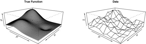
Figure 1: True regression function $m(x_{1},x_{2})$ (11) on the square $[0,1]\times[0,1]$ used in our numerical examples and a sample of size 100 with errors and a sample of 100 points

Figure 2 shows the evolution of the bias corrected smoother, starting from a nearly linear pilot smoother in panel (a). At iteration $k=500$ (or 499 iterative bias reduction steps), the smoother shown in panel (b) is visually close to the original regression function. Continuing the bias correction scheme will eventually lead to a smoother that interpolates the raw data. This example shows the importance of suitably selecting the number of bias correction iterations.

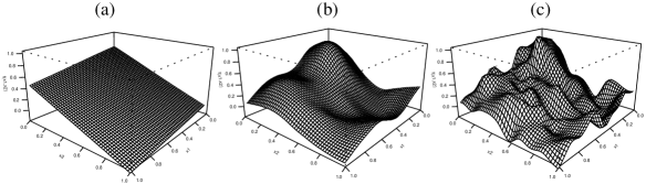
Figure 2: TPS regression smoothers from $100$ noisy observations from (11) (see Figure 1) evaluated on a regular grid on $[0,1]\times[0,1]$. Panel (a) shows the pilot smoother, panel (b) graphs the bias corrected smoother after 500 iterations and panel (c) graphs the smoother after 50000 iterations of the bias correction scheme.

3.2 Adaptation to smoothness of the regression function

Let $\Omega$ be an open bounded subset of $\mathbb{R}^{d}$ and suppose that the unknown regression function $m$ belongs to the Sobolev space $\mathcal{H}^{(\nu)}(\Omega)=\mathcal{H}^{(\nu)}$, where $\nu$ is an integer such that $\nu>d/2$. Let $S$ denote the smoothing matrix of a thin-plate spline of order $\nu_{0}\leq\nu$ (in practice we will take the smallest possible value $\nu_{0}=\lfloor d/2\rfloor+1$) and fix the smoothing parameter $\lambda_{0}>0$ to some reasonably large value. Our next theorem states that there exists a number of iterations $k=k(n)$, depending on the sample size, for which the resulting estimate $\widehat{m}_{k}$ achieves the optimal rate of convergence. In light of that theorem, we expect that an iterative bias corrected smoother, with the number of iterations selected by GCV, will achieve the optimal rate of convergence.

Theorem 1

Assume that the design $X_{i}\in\Omega$, $i=1,\ldots,n$ satisfies the following assumption: Define

$$h_{max}(n)=\sup_{x\in\Omega}\inf_{i=1,\ldots,n}|x-X_{i}|,\mbox{ and }h_{min}(n)=\min_{i\neq j}|X_{i}-X_{j}|,$$

and assume that there exists a constant $B>0$ such that

$$\frac{h_{max}(n)}{h_{min}(n)}\leq B\quad\forall n.$$

Suppose that the true regression function $m\in\mathcal{H}^{(\nu)}$.

If the initial estimator $\hat{m}_{1}=SY$ is obtained with $S$ a thin-plate spline of degree $\nu_{0}$, with $\lceil d/2\rceil\leq\nu_{0}<\nu$ and a fixed smoothing parameter $\lambda_{0}>0$ not depending on the sample size $n$, then there is an optimal number of iterations $k(n)$ such that the resulting smoother $\widehat{m}_{k}$ satisfies

$$\mathbb{E}\left[\left(\frac{1}{n}\sum_{j=1}^{n}(\hat{m}_{k}(X_{j})-m(X_{j})\right)^{2}\right]=O\left(n^{-2\nu/(2\nu+d)}\right),$$

which is the optimal rate of convergence for $m\in\mathcal{H}^{(\nu)}$.

While adaptation of the $L_{2}$-boosting algorithm applied to univariate smoothing splines was proven by Bühlmann and Yu (2003), the application of bias reduction to achieve adaptation to the smoothness of multivariate regression function has not been previously exploited. Rate optimality of the smoother $\hat{m}_{k}$ is achieved by suitable selection of the number of bias correcting iterations, while the smoothing parameter $\lambda_{0}$ remains unchanged. That is, the effective size of the neighborhoods the smoother averages over remains constant. Selecting the optimal number of iterations is important and we prove that result with GCV criterion using Theorem 3.2 of Li (1987).

Theorem 2

Let $\hat{k}_{GCV}\in\mathcal{K}_{n}=\{1,\ldots,\lfloor n^{\gamma}\rfloor\}$, $1\leq\gamma\leq(2\nu_{0})/d$, denote the index in the sequence of bias corrected smothers whose associated smoother minimize the generalized cross-validation criteria. Suppose that the noise $\varepsilon$ in (1) has finite $4q^{th}$ absolute moment, where $q>\gamma(2\nu/d+1)$, that is, ${\mathbb{E}}[|\varepsilon|^{4q}]<\infty$. Then as the sample size $n$ grows to infinity,

$$\frac{\|\hat{m}_{\hat{k}_{GCV}}-m\|^{2}}{\inf_{k\in\mathcal{K}_{n}}\|\hat{m}_{k}-m\|^{2}}\longrightarrow 1,\quad\hbox{in probability}.$$

The moment condition is satisfied for Gaussian or subgaussian errors.

4 Iterative bias reduction of kernel smoothers

The matrix $S$ of thin plate spline is symmetric and has eigenvalues in $(0,1]$ (see for example Utreras, 1988). In particular, the first $M_{0}={\nu_{0}+d-1\choose\nu_{0}-1}$ eigenvalues are all equal to one, corresponding to the parametric component of the smoothing spline. The sample size $n$ needs to be at least $M_{0}$, and since from Theorem 1 we want $\nu_{0}>d/2$, it follows that $M_{0}$ grows exponentially fast in the number of covariates $d$. In particular the dimension of the parametric component of freedom is $5,28,165,1001$ for $d=4,6,8,10$, respectively, and more generally, $M_{0}$ grows like $3^{d/2}\times(3/2)^{d}$ for large $d$. This feature limits the practical usefulness of TPS smoothers. For example, the regression model in Section 5 for the Boston housing data set that has $13$ covariates can not be fit with a TPS because its sample size $n=506<27500\approx M_{0}$.

A possible resolution to this problem is to approximate the TPS smoother with a kernel smoother, with an appropriate kernel (see Silverman, 1984; Messer, 1991). In this section, we discuss kernel based smoothers in general, and we give a necessary and sufficient condition on the kernel that ensures that the iterative bias correction scheme is well behaved. We supplement our theorems with numerical examples of both good and bad behavior of our scheme.

4.1 Kernel type smoothers

The matrix $S$ of kernel estimators has entries $S_{ij}=K(d_{h}(X_{i},X_{j}))/\sum_{k}K(d_{h}(X_{i},X_{j}))$, where $K(.)$ is typically a symmetric function in ${\mathbb{R}}$ (e.g., uniform, Epanechnikov, Gaussian), and $d_{h}(x,y)$ is a weighted distance between two vectors $x,y\in{\mathbb{R}}^{d}$. The particular choice of the distance $d(\cdot,\cdot)$ determines the shape of the neighborhood. For example, the weighted Euclidean norm

$$d_{h}(x,y)=\sqrt{\sum_{j=1}^{d}\frac{(x_{j}-y_{j})^{2}}{h_{j}^{2}}},$$

where $h=(h_{1},\ldots,h_{d})$ denotes the bandwidth vector, gives rise to elliptic neighborhoods.

4.2 Spectrum of kernel smoothers

While the smoothing matrix $S$ is not symmetric, it has a real spectrum. Write $S=D\mathbb{K}$, where $\mathbb{K}$ is symmetric matrix with general element ${\mathbb{K}}_{ij}=K(d_{h}(X_{i},X_{j}))$ and $D$ is diagonal matrix with elements $D_{ii}=1/\sum_{j}K(d_{h}(X_{i},X_{j}))$. If $q$ is an eigenvector of $S$ associated to the eigenvalue $\lambda$, then

$$Sq=D{\mathbb{K}}q=D^{1/2}\left(D^{1/2}{\mathbb{K}}D^{1/2}\right)D^{-1/2}q=\lambda q,$$

and hence

$$\left(D^{1/2}{\mathbb{K}}D^{1/2}\right)\left(D^{-1/2}q\right)=\lambda\left(D^{-1/2}q\right).$$

Hence the symmetric matrix $A=D^{1/2}{\mathbb{K}}D^{1/2}$ has the same spectrum as $S$. Since $S$ is row-stochastic, all its eigenvalues are bounded by one. Thus, in light of Theorem 1, we seek conditions on the kernel $K$ to ensure that its spectrum is non-negative. Necessary and sufficient conditions on the smoothing kernel $K$ for $S$ to have a non-negative spectrum are given in the following Theorem.

Theorem 3

If the inverse Fourier-Stieltjes transform of a kernel $K(\cdot)$ is a real positive finite measure, then the spectrum of the Nadaraya-Watson kernel smoother lies between zero and one.

Conversely, suppose that $X_{1},\ldots,X_{n}$ are an independent $n$-sample from a density $f$ (with respect to Lebesgue measure) that is bounded away from zero on a compact set strictly included in the support of $f$. If the inverse Fourier-Stieltjes transform of a kernel $K(\cdot)$ is not a positive finite measure, then with probability approaching one as the sample size $n$ grows to infinity, the maximum of the spectrum of $I-S$ is larger than one.

Remark 1: The assumption that the inverse Fourier-Stieltjes transform of a kernel $K(\cdot)$ is a real positive finite measure is equivalent to the kernel $K(\cdot)$ being positive-definite function, that is, for any finite set of points $x_{1},\ldots,x_{m}$, the matrix

$$\left(\begin{array}[]{ccccc}K(0)&K(d_{h}(x_{1},x_{2}))&K(d_{h}(x_{1},x_{3}))&\dots&K(d_{h}(x_{1},x_{m}))\\ K(d_{h}(x_{2},x_{1}))&K(0)&K(d_{h}(x_{2},x_{3}))&\dots&K(d_{h}(x_{2},x_{m}))\\ \vdots&&&&\vdots\\ K(d_{h}(x_{m},x_{1}))&K(d_{h}(x_{m},x_{2}))&K(d_{h}(x_{m},x_{3}))&\dots&K(0)\end{array}\right)$$

is positive definite. We refer to Schwartz (1993) for a detailed study of positive definite functions.

Remark 2: Di Marzio and Taylor (2008) proved the first part of the theorem in the context of univariate smoothers. Our proof of the converse shows that for large enough sample sizes, most configurations from a random design lead to smoothing matrix $S$ with negative singular values.

Iterative smoothing of the residuals can be computationally burdensome. To derive an alternative, and computationally more efficient representation of the iterative bias corrected smoother, observe that

$$\hat{m}_{k} = [I-D^{1/2}(I-D^{1/2}\mathbb{K}D^{1/2})^{k}D^{-1/2}]Y$$

$$= D^{1/2}[I-(I-A)^{k}]D^{-1/2}Y.$$

Writing $A=D^{1/2}\mathbb{K}D^{1/2}=P_{A}\Lambda_{A}P_{A}^{t}$, where $P_{A}$ is the orthonormal matrix of eigenvectors and $\Lambda_{A}$ diagonal matrix of their associated eigenvalues, we obtain a computationally efficient representation for the smoother

$$\hat{m}_{k} = D^{1/2}P_{A}[I-(I-\Lambda_{A})^{k}]P_{A}^{t}D^{-1/2}Y.$$

Note that the eigenvalue decomposition of $A$ needs only to be computed once, and hence leads to a fast implementation for calculating the sequence of bias corrected smoothers.

The Gaussian and triangular kernels are positive definite kernels (they are the Fourier transform of a finite positive measure, (Feller, 1966)). In light of Theorem 3, the iterative bias correction of Nadaraya-Watson kernel smoothers with these kernels produces a sequence of well behavior smoother.

The anticipated behavior of iterative bias correction for Gaussian kernel smoothers is confirmed in our numerical example. Figure 3 shows the progression of the sequence of bias corrected smoothers starting from a very smooth surface (see panel (a)) that is nearly constant. Fifty iterations (see panel (b)) produces a fit that is visually similar to the original function. Continued bias corrections then slowly degrades the fit as the smoother starts to over-fit the data. Continuing the bias correction scheme will eventually lead to a smoother that interpolates the data. This example hints at the potential gains that can be realized by suitably selecting the number of bias correction steps.

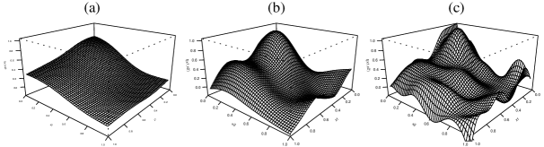
Figure 3: Gaussian kernel smoother of $m(x_{1},x_{2})$ from $n=100$ equidistributed points on $[0,1]\times[0,1]$, evaluated on a regular grid with (a) $k=1$, (b) 50 and (c) 10000 iterations.

The uniform and the Epanechnikov kernels are not positive definite. Theorem 3 states that for large enough samples, we expect with high probability that $I-S$ has at least one eigenvalue larger than one. When this occurs, the sequence of iterative bias corrected smoothers will behave erratically and eventually diverge. Proposition 2 below strengthens this result by giving an explicit condition on the configurations of the design points for which the largest singular value of $I-S$ is always larger than one.

Proposition 2

Denote by ${\mathcal{N}}_{i}$ the following set: $\{X_{j}:K(d_{h}(X_{j},X_{i}))>0\}$.

If there exists a set ${\mathcal{N}}_{i}$ which contains (at least) two points $X_{j},X_{k}$ different of $X_{i}$ such that $d_{h}(X_{i},X_{j})<1$, $d_{h}(X_{i},X_{k})<1$ and $d_{h}(X_{j},X_{k})>1$, then the smoothing matrix $S$ for the uniform kernel smoother has at least one negative eigenvalue.

If there exits a set ${\mathcal{N}}_{i}$ that contains (at least) two points $X_{j},X_{k}$ ifferent of $X_{i}$ that satisfy

$$d_{h}(X_{j},X_{k})>\min\{d_{h}(X_{i},X_{j}),d_{h}(X_{i},X_{k})\},$$

then the smoothing matrix $S$ for the Epanechnikov kernel smoother has at least one negative eigenvalue.

The failure of the iterated bias correction scheme using Epanechnikov kernel smoothers is illustrated in the numerical example shown in Figure 4. As for the Gaussian smoother, the initial smoother (panel (a)) is nearly constant. After five iterations (panel (b)) some of the features of the function become visible. Continuing the bias corrections scheme produces an unstable smoother. Panel (c) shows that after only 25 iterations, the smoother becomes noisy. Nevertheless, when comparing panel (a) with panel (b), we see that some improvement is possible from a few iterations of the bias reduction scheme.

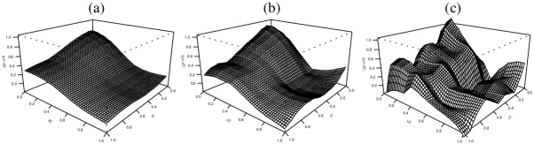
Figure 4: Epanechnikov kernel smoother of $m(x_{1},x_{2})$ from $n=100$ equidistributed points on $[0,1]\times[0,1]$, evaluated on a regular grid with (a) $k=1$, (b) 5 and (c) 25 iterations.

5 Simulations and a real example

This section presents the results of a modest simulation study to compare the empirical mean squared error

$$MSE = \frac{1}{n}\sum_{i=1}^{n}(\hat{m}(X_{i})-m(X_{i}))^{2}$$ (12)

of our procedure to its competitors for two functions, in dimensions $d=3,5,7$ and sample sizes $n=50,100,200,500,800$, with a noise to signal ratio of $10\%$. In order to exploit our theoretical result, the pilot smoother has to oversmooth otherwise the pilot smoother will have no bias and our iterative debiasing procedure has no more justification. So starting with a small $\lambda$ will lead to zero or a small number of iterations. Oppositely, starting with a big $\lambda$ will normally lead to a large number of iterations. We decide in this section to use the values by default in the ibr R-package. The thin plate spline is govern by a single parameter $\lambda$ that weights the contribution of the roughness penalty. For estimating a $d$-valued regression function, the parametric component is $M_{0}={\nu_{0}+d-1\choose\nu_{0}-1}$ and we choose $\lambda$ such that the initial degree of freedom of the pilot smoother equals equals $1.5M_{0}$. The implementation for the kernel smoother is different since we could choose a different bandwidth for each explanatory variables. We choose one bandwidth for each explanatory variable $X_{i}$ such as the effective degree of freedom for the one-dimensional smoothing matrix related to $X_{i}$ has a trace equal to 1.1 (more degree than a constant but less than a linear model). For such values, the pilot smoothers always oversmooth.

Our simulations was designed to allow us to investigate three aspects: First, compare the performance of the thin plate spline with smoothing parameter selected by GCV with the IBR smoother using a thin plate spline with a large smoothing parameter. We expect that adaptation of our method will translate into a better performance of our smoother over the optimal TPS smoother. Second, to compare the performance between IBR smoother using either TPS and kernel based smoothers. Since kernel smoothers do not have a parametric component (which may, or may not, be needed to fit the data), we believe that kernel smoothers use more effectively their degree of freedom, which translates into better performance. Third, we want to compare the performance of fully nonparametric smoothers and additive smoothers. While with additive models we estimate an approximation of the true regression function, it is generally believed that the approximation error of an additive model is smaller than the estimation error of a fully multivariate smoother even for dimensions for small sample sizes, e.g. $n=50,100$, and moderate dimensions of the covariates, e.g. $d=5$. The results of our study are summarized in Table 1 and Figure 5.

Figure 5 shows nine panels each containing the boxplots of the MSE from 500 simulations, on a logarithmic scale on the $y$-axis. Moving from top to bottom ranges the regression functions from the function of three variables $\sin(2\pi(x_{1}x_{2})^{1/2})+\cos(2\pi(x_{2}x_{3})^{1/2})$, to the function of five variables $\sin(2\pi(x_{1}x_{2}x_{3})^{1/3})+\cos(2\pi(x_{3}x_{4}x_{5})^{1/3})$ and to the function of seven variables $\sin(2\pi(x_{1}x_{2}x_{3}x_{4})^{1/4})+\cos(2\pi(x_{4}x_{5}x_{6}x_{7})^{1/4})$. All the covariates are i.i.d. uniforms on the interval $(1,2)$. Moving from left to right changes the sample size from $n=50,200,800$. Within each panel, the boxplot of MSE is shown, in the order from left to right, of additive models using the function gam from the R package mgcv , TPS with optimal smoothing parameter using the function Tps from the R package fields, iterative bias reduction with TPS smoother using the function ibr from the ibr R package and iterative bias reduction with kernel smoothers, using again the ibr function. For reasons explained in Section 4, no TPS smoothers can be evaluated for the $d=7$, $n=50$ panel.

Figure 5 shows that a fully nonparametric smoother is always preferred to an additive smoother, even for relative small sample sizes and moderate dimensions.

Figure 5: Boxplot of Mean Squared Error (MSE) of smoothers for the regression functions (from top to bottom) of three variables $\sin(2\pi(x_{1}x_{2})^{1/2})+\cos(2\pi(x_{2}x_{3})^{1/2})$, five variables $\sin(2\pi(x_{1}x_{2}x_{3})^{1/3})+\cos(2\pi(x_{3}x_{4}x_{5})^{1/3})$ and seven variables $\sin(2\pi(x_{1}x_{2}x_{3}x_{4})^{1/4})+\cos(2\pi(x_{4}x_{5}x_{6}x_{7})^{1/4})$, and of sample size (from left to right) of $n=50,200,800$. Each panel shows the boxplot of the MSE of a GAM smoother, TPS smoother, IBR with TPS smoother and IBR with kernel smoother.

In extensive simulations, to be reported in a follow-on paper, we observe that this qualitative conclusion holds over a wide variety of regression functions. Generally, as expected, the TPS with optimal smoothing parameter has a somewhat worse performance than the TPS IBR smoother. And finally, the kernel based IBR smoother is slightly better than the TPS based IBR smoother, especially in higher dimensions.

Table 1 gives further insight into the performance of the various smoothers. Our table presents the ratio of the median MSE (in 500 simulation runs) of various smoothers to the median MSE of the kernel based IBR smoother. Since all the entries are larger than one, we conclude that kernel based IBR consistently outperforms the other smoothing procedures over the range of sample size, number of covariates and regression functions we considered in our study.

function	$n$	gam	tps	ibr-tps	ibr-k
	50	2.59	1.63	1.39	1
	100	4.59	1.89	1.58	1
$x_{1}x_{2}x_{3}$	200	8.38	2.14	1.73	1
	500	17.9	2.56	2.08	1
	800	27.4	2.82	2.39	1
	50	6.72	1.70	1.09	1
	100	12.0	1.80	1.19	1
$\sin(2\pi(x_{1}x_{2})^{1/2})+\cos(2\pi(x_{2}x_{3})^{1/2})$	200	22.3	1.91	1.27	1
	500	46.2	1.99	1.45	1
	800	67.3	2.04	1.51	1
	50	2.16	1.60	1.47	1
	100	3.83	1.42	1.39	1
$x_{1}x_{2}x_{3}x_{4}x_{5}$	200	6.64	1.28	1.24	1
	500	13.17	1.24	1.22	1
	800	19.44	1.26	1.23	1
	50	3.62	1.26	1	1
	100	6.32	1.76	1.15	1
$\sin(2\pi(x_{1}x_{2}x_{3})^{1/3})+\cos(2\pi(x_{3}x_{4}x_{5})^{1/3})$	200	10.0	1.95	1.31	1
	500	18.6	2.06	1.38	1
	800	26.5	2.18	1.46	1
	50	2.05	-	-	1
	100	3.11	-	-	1
$x_{1}x_{2}x_{3}x_{4}x_{5}x_{6}x_{7}$	200	5.26	3.53	3.17	1
	500	9.85	2.46	2.45	1
	800	13.8	2.07	2.07	1
	50	3.16	-	-	1
	100	4.38	-	-	1
$\sin(2\pi(x_{1}x_{2}x_{3}x_{4})^{1/4})+\cos(2\pi(x_{4}x_{5}x_{6}x_{7})^{1/4})$	200	6.43	1.78	1.57	1
	500	11.1	1.37	1.31	1
	800	14.9	1.27	1.22	1

Table 1: Ratio of median MSE over 500 simulations of a smoother and the median MSE over 500 simulations of the kernel based IBR smoother. The smoothers, from left to right, are Generalized Additive Model (GAM), TPS with optimally selected smoothing parameter (tps), TPS based IBR (ibr-tps) and kernel based IBR (ibr-k).

The improvement over a GAM model ranges from 100% to 6000%. This reinforces our conclusions that fully nonparametric regressions are practical for moderately large number of covariates, even for sample sizes as small as $n=50$.

The other notable observation is that the values in the ibr-tps column are always less than those in the tps column, showing that consistently, the TPS based IBR smoother has better performance than TPS with optimal smoothing parameter. In our simulation study, the typical improvement is of 20%.

5.1 Boston housing data

We apply our method on the Boston housing data. This dataset, created by Harrison and Rubinfeld (1978) has been extensively to showcase the performance and behavior of nonparametric multivariate smoothers, see for example Breiman and Friedman (1995) and more recently by Di Marzio and Taylor (2008). The data contains 13 explanatory variables describing each of 506 census tracts in the Boston area taken from the 1970 census, together with the median value of owner-occupied homes in $1000’s. The sample size of the data is $n=506$ and the number of explanatory variables $d=13$.

We compare our method with the MARS algorithm of Friedman (1991) as implemented in the R package mda, with projection pursuit regression (function ppr), additive models using the backfitting algorithm of Hastie and Tibshirani (1995) as implemented in the R package mgcv, and additive Boosting Bühlmann and Yu (2003) from the R package mboost.

The predicted mean squared error is estimated by randomly splitting 30 times the data into training sets (size $n=350$) and testing sets ($n=156$). We summarize the results of our analysis in the following table:

Table 2: Predicted mean Squared Error on test observations for Boston housing data.

Method	Mean Predicted Squared Error
Multivariate regression	20.09
$L_{2}$Boost with component-wise spline	9.59
additive model (backfitted with R)	11.77
Projection pursuit (with R)	12.64 (4)
MARS (with R)	10.54
IBR with GCV stopping rule
and multivariate Gaussian kernel with
1.1 initial DDL per variable and 1230 iterations	7.35

Table 2 again supports our claim that the fully multivariate method presented in the paper leads to a reduction of more than 30% in the prediction mean squared error over competing state-of-the-art multivariate smoothing methods. A similar comparison for responses on the logarithmic scale reveals the even larger reduction of 40% in the prediction mean squared error. Since our fully nonparametric regression smoother has substantially smaller prediction error over additive linear models and low-order interaction models, we conclude that there exist higher order interactions in that data that are significant.

6 Conclusion

This paper introduces a fully multivariate regression smoother for estimating the regression function $m(X_{1},\ldots,X_{d})$ obtained by successive bias correction from a very smooth (biased) pilot smoother. We show that the resulting smoother is adaptive to the underlying smoothness (see theorems 1 and 2). This adaptation to the underlying smoothness partially mitigates the effect from the curse of dimensionality in many practical examples, and make it practical to use fully nonparametric smoother in moderate dimensions, even for smaller sample sizes.

As in $L_{2}$ boosting, the proposed iterative bias correction scheme needs a weak learner as a base smoother $S$, but all weak learners are not suitable (see theorem 1). For instance, Epanechnikov kernel smoothers are not interesting (see Theorem 3). We further note that one does not need to keep the same smoother throughout the iterative bias correcting scheme. We conjecture that there are advantages to using weaker smoothers later in the iterative scheme, and shall investigate this in a forthcoming paper.

Finally, the R package ibr available at CRAN implements the proposed multivariate nonparametric method in R.

Appendix

Proof of Proposition 1

$$\|\hat{b}_{k}\|^{2} = \|-(I-S)^{k-1}SY\|^{2}$$

$$= \|(I-S)(I-S)^{k-2}SY\|^{2}\leq\|(I-S)\|^{2}\|\hat{b}_{k-1}\|^{2}$$

$$\leq \|\hat{b}_{k-1}\|^{2},$$

where the last inequality follows from the assumptions on the spectrum of $I-S$.
Proof of Theorem 1 Let $\nu_{0}<\nu$ and fix the smoothing parameter $\lambda_{0}$. Define $S=S_{\nu_{0},\lambda_{0}}$. The eigen decomposition of $S$ [Utreras, 1988] gives

$$\lambda_{1}=\cdots=\lambda_{M_{0}}=1\quad\hbox{and}\quad\frac{\alpha_{j}}{1+\lambda_{0}j^{2\nu_{0}/d}}\leq\lambda_{j}\leq\frac{\beta_{j}}{1+\lambda_{0}j^{2\nu_{0}/d}},$$

where $M_{0}=\choose{}^{d+\nu_{0}-1}_{\nu_{0}-1}$ and $\alpha_{j}$ and $\beta_{j}$ are two positive constants. We decide to simplify the notation using

$$\lambda_{j}\approx\frac{1}{1+\lambda_{0}j^{2\nu_{0}/d}}$$

Let us evaluate the variance of the estimator:

$$V(\hat{m}_{k},\lambda_{0},\nu_{0}) \approx \sigma^{2}\frac{M_{0}}{n}+\frac{\sigma^{2}}{n}\sum_{j=M_{0}+1}^{n}\left[\left(1-(1-\frac{1}{1+\lambda_{0}j^{2\nu_{0}/d}})^{k}\right)\right]^{2}.$$

Choose $J_{n}$ in $j=M_{0},\ldots,n$, and split the sum in two parts. Then bound the summand of the first sum by one to get

$$V(\hat{m}_{k},\lambda_{0},\nu_{0}) \leq \sigma^{2}\frac{M_{0}}{n}+\sigma^{2}\frac{J_{n}-M_{o}}{n}+\frac{\sigma^{2}}{n}\sum_{j=J_{n}+1}^{n}\left[\left(1-(1-\frac{1}{1+\lambda_{0}j^{2\nu_{0}/d}})^{k}\right)\right]^{2}.$$

As the function $1-(1-u)^{k}\leq ku$ for $u\in[0,1]$, we have

$$V(\hat{m}_{k},\lambda_{0},\nu_{0}) \leq \sigma^{2}\frac{J_{n}}{n}+k^{2}\frac{\sigma^{2}}{n}\sum_{j=J_{n}+1}^{n}\left(\frac{1}{1+\lambda_{0}j^{2\nu_{0}/d}}\right)^{2}$$

$$\leq \sigma^{2}\frac{J_{n}}{n}+k^{2}\frac{\sigma^{2}}{n}\sum_{j=J_{n}+1}^{n}\frac{1}{\lambda_{0}^{2}j^{4\nu_{0}/d}}.$$

Bounding the sum by the integral and evaluate the latter, one has

$$V(\hat{m}_{k},\lambda_{0},\nu_{0}) \leq \sigma^{2}\frac{J_{n}}{n}+k^{2}\frac{\sigma^{2}}{n}\frac{1}{\lambda^{2}(4\nu_{0}/d-1)}J_{n}^{-4\nu_{0}/d+1}.$$

If we want to balance the two terms of the variance, one has to choose the following number of iterations $K_{n}=O(J_{n}^{2\nu_{0}/d})$. For such a choice the variance is of order

$$V(\hat{m}_{k},\lambda_{0},\nu_{0}) = O\left(\frac{J_{n}}{n}\right).$$

Let us evaluate the squared bias of $\hat{m}_{k}$. Recall first the decomposition of $S_{\nu_{0},\lambda_{0}}=P_{\nu_{0}}\Lambda P^{\prime}_{\nu_{0}}$ and denote by $\mu_{j,\nu_{0}}=[P^{\prime}_{\nu_{0}}]_{j}m$ the coordinate of $m$ in the eigen vector space of $S_{\nu_{0},\lambda_{0}}$.

$$b(\hat{m}_{k},\lambda_{0},\nu_{0}) = \frac{1}{n}\sum_{j=1}^{n}\left(1-\lambda_{j}\right)^{2k}\mu_{j,\nu_{0}}^{2}$$

$$= \frac{1}{n}\sum_{j=M_{0}+1}^{j_{n}}\left(1-\lambda_{j}\right)^{2k}\mu_{j,\nu_{0}}^{2}+\frac{1}{n}\sum_{j=j_{n}+1}^{n}\left(1-\lambda_{j}\right)^{2k}\mu_{j,\nu_{0}}^{2}$$

If $m$ belongs to $\mathcal{H}^{(\nu)}$ it belongs to $\mathcal{H}^{(\nu_{0})}$ and we have the following relation by property of $\mathcal{H}^{(\nu_{0})}$

$$\frac{1}{n}\sum_{j=M_{0}+1}^{n}j^{2\nu_{0}/d}\mu_{j,\nu_{0}}^{2}\leq M<\infty.$$ (13)

Using the fact that $\lambda_{j}>0$, we have:

$$b(\hat{m}_{k},\lambda_{0},\nu_{0}) \leq \frac{1}{n}\sum_{j=M_{0}+1}^{j_{n}}j_{n}^{-2\nu/d}j_{n}^{2\nu/d}\mu_{j,\nu_{0}}^{2}+\frac{1}{n}\sum_{j=j_{n}+1}^{n}j^{-2\nu/d}j^{2\nu/d}\mu_{j,\nu_{0}}^{2}$$

$$b(\hat{m}_{k},\lambda_{0},\nu_{0}) \leq j_{n}^{-2\nu/d}\sum_{j=M_{0}+1}^{j_{n}}j_{n}^{2\nu/d}\mu_{j,\nu_{0}}^{2}+j_{n}^{-2\nu/d}\frac{1}{n}\sum_{j=j_{n}+1}^{n}j^{2\nu/d}\mu_{j,\nu_{0}}^{2}$$

Using the same type of bound as in equation (13) we get

$$b(\hat{m}_{k},\lambda_{0},\nu_{0}) \leq j_{n}^{-2\nu/d}M^{\prime}+j_{n}^{-2\nu/d}M^{\prime\prime}.$$

Thus the bias is of order $O(j_{n}^{-2\nu/d})$.
Balancing the squared bias and the variance lead to the choice

$$J_{n} = O(n^{1/(1+2\nu/d)})$$

and we obtain the desired optimal rate.


Proof of Theorem 2 We show that conditions (A.1) to (A.7) given by Li [1987], in theorem 3.2 are satisfied. To make the proof self contained, we recall briefly these conditions: $(A.1)\ \lim_{n\rightarrow\infty}\sup_{k\in\mathcal{K}_{n}}\lambda(S_{k})<\infty,\ \ (A.2)\ E(\varepsilon^{4m})<\infty,\ \ (A.3)\ \sum_{k\in\mathcal{K}_{n}}(nR_{n}(k))^{-m}\rightarrow 0,$
where $R_{n}(k)=\mathbb{E}(\|m_{n}-\hat{m}_{k,n}\|^{2})/n$,   $(A.4):\inf_{k\in\mathcal{K}_{n}}n^{-1}\|\hat{m}_{k}-m\|^{2}\rightarrow 0,$ in probability.
$(A.5)$ for any sequence $\{k_{n}\in\mathcal{K}_{n}\}$ such that $n^{-1}\mathrm{trace}(S_{k_{n}}S^{\prime}_{k_{n}})\rightarrow 0$ we have
$\{n^{-1}\mathrm{trace}(S_{k_{n}})\}^{2}/\{n^{-1}\mathrm{trace}(S_{k_{n}}S^{\prime}_{k_{n}})\}\rightarrow 0,$ $(A.6)\ \sup_{k\in\mathcal{K}_{n}}n^{-1}\mathrm{trace}(S_{k})\leq\gamma_{1}\mbox{ for some }1>\gamma_{1}>0,$
$(A.7)\ \sup_{k\in\mathcal{K}_{n}}\{n^{-1}\mathrm{trace}(S_{k})\}^{2}/\{n^{-1}\mathrm{trace}(S_{k}S^{\prime}_{k})\}\leq\gamma_{2}\mbox{ for some }1>\gamma_{2}>0.$

Conditions (A.1) to (A.4)
The eigen values of $S_{k}$ (denoted as $\lambda(S_{k})$) are between 0 and 1 $\forall n$, thus the condition (A.1) is fulfilled. To fulfill condition (A.3) we need to calculate $\sum_{k\in\mathcal{K}_{n}}nR_{n}(k)^{-m}$, where $m$ is an integer to be found, $m_{n}=(m(X_{1}),\ldots,m(X_{n}))^{\prime}$ and $\hat{m}_{k,n}=S_{k}Y$. Using Theorem 1 we have that for an optimal choice of $k$, $R_{n}(k)=\mathcal{O}(n^{d/(2\nu+d)})$. Let us choose $\mathcal{K}_{n}$ such that its cardinal is of order $n^{\gamma}$ ($1\leq\gamma\leq(2\nu_{0})/d$), we get the order of an upper bound of $\sum_{k\in\mathcal{K}}nR_{n}(k)^{-m}$ is $n^{\gamma-\frac{md}{2\nu+d}}$. To have (A.3) fulfilled we need that $\gamma-\frac{md}{2\nu+d}<0$, that is $m>\gamma(2\nu/d+1)$. Condition (A.4) is satisfied because of Theorem 1.

Conditions (A.5) to (A.7) are related the trace of the matrix $S_{k}$ and of $S_{k}^{2}$. Let us recall first some general remarks

$$\frac{1}{n}\mathrm{trace}(S_{k}) = \frac{1}{n}\left(M_{0}+\sum_{j=M_{0}+1}^{n}\left[1-(1-\lambda_{j})^{k}\right]\right)$$

where the eigen values $\lambda_{j}$ are less than 1, bigger than 0 and decreasing. So $\mathrm{trace}(S_{k})$ and $\mathrm{trace}(S_{k}^{2})$ are increasing with $k$. By proposition 1, $\lim_{k_{n}\rightarrow\infty}\left(\frac{1}{n}\mathrm{trace}(S_{k_{n}})\right)=1$ and the same is true for $\mathrm{trace}(S_{k_{n}}^{2})$ so the choice of the maximal value of $k_{n}$ is important as it will be emphasize in the proof. The last general remark is the following

$$\left(\frac{1}{n}\mathrm{trace}S_{k}\right)^{2}\leq\frac{1}{n}\mathrm{trace}S_{k}^{2}\leq\frac{1}{n}\mathrm{trace}S_{k}\leq 1.$$

Thanks to Utreras [1988], we know that

$$\lambda_{j} \approx \frac{1}{1+\lambda_{0}j^{\alpha_{0}}},\quad\alpha_{0}=\frac{2\nu_{0}}{d}>1.$$

Let us write

$$(1-\lambda_{j})^{k} = \left[\frac{\lambda_{0}j^{\alpha_{0}}}{1+\lambda_{0}j^{\alpha_{0}}}\right]^{k}=\left(1+\lambda_{0}^{-1}j^{-\alpha_{0}}\right)^{-k}$$

So we have

$$\frac{1}{n}\mathrm{trace}(S_{k}) \approx \frac{1}{n}M_{0}+\frac{1}{n}\sum_{j=M_{0}+1}^{n}\left(1-\left[1+\lambda_{0}^{-1}j^{-\alpha_{0}}\right]^{-k}\right)$$

$$\approx \frac{1}{n}M_{0}+\sum_{j=M_{0}+1}^{n}g_{k}(j).$$

We can write

$$g_{k}(j_{n}) = 1-\left[1+\lambda_{0}^{-1}j_{n}^{-\alpha_{0}}\right]^{-k}$$

$$= 1-\exp{[-k\ln{(1+\lambda_{0}^{-1}j_{n}^{-\alpha_{0}})}]}$$

$$= 1-\exp{[-k\lambda_{0}^{-1}j_{n}^{-\alpha_{0}}]}.$$

Let us consider the case where $j_{n}$ tends to infinity. We want to ensure the following condition: $-k_{n}j_{n}^{-\alpha_{0}}$ tends to zero. Since $k_{n}=n^{\gamma}$ consider $\varepsilon>0$ such that $\varepsilon<\alpha_{0}-\gamma$ and assume that

$$j_{n}=O(n^{(\gamma+\varepsilon)/\alpha_{0}}),$$

then $-k\lambda_{0}^{-1}j_{n}^{-\alpha_{0}}\rightarrow 0$ even when $k$ is at maximum rate of order $n^{\gamma}$. Thus when $n$ grows to infinity, $\forall j\geq j_{n}$ we have the following approximation for $g_{k}(j)$:

$$g_{k}(j)\approx kj^{-\alpha_{0}}\lambda_{0}^{-1}.$$ (14)

Order of an upper bound of $\mathrm{trace}(S_{k})/n$
$\forall k\in\mathcal{K}_{n}$, we have when $n$ grows to infinity:

$$\frac{1}{n}\mathrm{trace}(S_{k}) \approx \frac{M_{0}}{n}+\frac{1}{n}\sum_{j=M_{0}+1}^{j_{n}}{g_{k}(j)}+\frac{1}{n}\sum_{j=j_{n}+1}^{n}{g_{k}(j)}$$

$$\leq \frac{j_{n}}{n}+\frac{1}{n}\int_{j_{n}}^{n}g_{k}(j)dj$$

$$\leq \frac{j_{n}}{n}+\frac{kj_{n}^{1-\alpha_{0}}}{n(\alpha_{0}-1)}\lambda_{0}^{-1}$$

with the last approximation which follows from equation (14). Using the fact that the maximum rate for $k_{n}$ is $O(n^{\gamma})$ and that $(\gamma,\varepsilon)$ are chosen such that $\gamma+\varepsilon<\alpha_{0}$ we have that an upper bound of $\mathrm{trace}(S_{k})/n$ is of order of $n^{\frac{\gamma+\varepsilon}{\alpha_{0}}-1}$.

Order of a lower bound of $\mathrm{trace}(S_{k}^{2})/n$
$\forall k\in\mathcal{K}_{n}$, we have when $n$ grows to infinity:

$$\frac{1}{n}\mathrm{trace}(S_{k}^{2}) \approx \frac{M_{0}}{n}+\frac{1}{n}\sum_{j=M_{0}+1}^{j_{n}}{g_{k}^{2}(j)}+\frac{1}{n}\sum_{j=j_{n}+1}^{n}{g_{k}^{2}(j)}$$

$$\geq \frac{M_{0}}{n}+\frac{g_{k}^{2}(j_{n})}{n}(j_{n}-M_{0})+\frac{1}{n}\int_{j_{n}+1}^{n+1}g^{2}_{k}(j)dj$$

$$\approx \frac{M_{0}}{n}+\frac{j_{n}-M_{0}}{n}g_{k}^{2}(j)+\frac{k^{2}\lambda_{0}^{-2}}{n}\frac{(j_{n}+1)^{-2\alpha_{0}+1}}{2\alpha_{0}-1}-\frac{k^{2}\lambda_{0}^{-2}}{n}\frac{(n+1)^{-2\alpha_{0}+1}}{2\alpha_{0}-1}$$

with the last approximation which follows from equation (14). Using one more time equation (14) we get that a lower bound of $\frac{1}{n}\mathrm{trace}(S_{k}^{2})$ if of order of $k^{2}n^{\frac{\gamma+\varepsilon}{\alpha_{0}}-1-2\varepsilon-2\gamma}$.

Condition (A.5)
Using the previous calculated order, we get that the order of $(\mathrm{trace}(S_{k})/n)^{2}(\mathrm{trace}(S_{k}^{2})/n)^{-1}$ is of order $k^{-2}n^{\frac{\gamma+\varepsilon}{\alpha_{0}}-1+2\varepsilon+2\gamma}$. Recall that $(\gamma,\varepsilon)$ are chosen such that $\gamma+\varepsilon<\alpha_{0}$, thus provided that $\varepsilon<1$ the condition (A.5) of Li’s theorem are fulfilled.

Condition (A.6)
The $n$ eigen values are decreasing. Consider now, $j_{n}=n\zeta$ with $\zeta$ fixed and less than one. We have that the maximal value of the mean of the trace which occurs at $k_{n}=n^{\gamma}$ is bounded by

$$\frac{1}{n}\mathrm{trace}(S_{k}) \leq \frac{j_{n}}{n}+\frac{(n-j_{n})}{n}k_{n}j_{n}^{-\alpha_{0}},$$

We can easily show that the last quantity is less than a given value smaller than 1. The aim of setting $k_{n}$ equal to $n^{\gamma}$ is to ensure that at the border of grid $\mathcal{K}_{n}$, the smoother is not identity (ie interpolating). When the smoother is too close to the identity matrix, conditions A.6 and A.7 are not fulfilled anymore. Moreover, being very close to identity is not interesting in a statistical viewpoint.

Condition (A.7)
We want to analyze

$$\sup_{k\in\mathcal{K}_{n}}\frac{\left(n^{-1}\mathrm{trace}(S_{k})\right)^{2}}{n^{-1}\mathrm{trace}(S_{k}^{2})}$$

Denote by

$$\alpha_{j}(k) = \ln(1-(1-\lambda_{j})^{k}),$$

so we have

$$\frac{1}{n}\mathrm{trace}S_{k} = \frac{1}{n}\sum_{j}\exp{\alpha_{j}(k)}$$

$$\frac{1}{n}\mathrm{trace}S_{k}^{2} = \frac{1}{n}\sum_{j}\exp{2\alpha_{j}(k)}$$

Let us show that the ratio is an increasing sequence in $k$. Let us evaluate the sign of the derivative of the ratio. We want to evaluate the sign of

$$\sum\!\exp{\alpha_{j}(k)}\sum\!\alpha^{\prime}_{j}(k)\exp{\alpha_{j}(k)}\sum\!\exp{2\alpha_{j}(k)}\!\!-\!\!\sum\!\exp{\alpha_{j}(k)}\sum\!\exp{\alpha_{j}(k)}\sum\!\alpha^{\prime}_{j}(k)\exp{2\alpha_{j}(k)}.$$

Simplifying and dividing by $\sum\exp{\alpha_{j}(k)}\sum\exp{2\alpha_{j}(k)}$ leads to

$$\frac{\frac{1}{n}\sum\alpha^{\prime}_{j}(k)\exp{\alpha_{j}(k)}}{\frac{1}{n}\sum\exp{\alpha_{j}(k)}}-\frac{\frac{1}{n}\sum\alpha^{\prime}_{j}(k)\exp{2\alpha_{j}(k)}}{\frac{1}{n}\sum\exp{2\alpha_{j}(k)}}$$

Rewrite as

$$\sum\alpha^{\prime}_{j}(k)\frac{\beta_{j}(k)}{\sum\beta_{j}(k)}-\sum\alpha^{\prime}_{j}(k)\frac{\beta_{j}(k)^{2}}{\sum\beta_{j}(k)^{2}}$$ (15)

The $\{\beta_{j}(k)\}_{j}$ is an increasing sequence bounded by one. It is possible to show that 15 is positive using induction. The maximum of the quantity under consideration grid $\mathcal{K}_{n}$ is obtained at the border of the grid. Condition (A.7) can be shown to be fulfilled by using upper bound of $\mathrm{trace}(S_{k})/n$ and lower bound $\mathrm{trace}(S^{2}_{k})/n$.
 
Proof of Theorem 3 For notational simplicity, we present the proof in the univariate case. Let $X_{1},\ldots,X_{n}$ is an i.i.d. sample from a density $f$ that is bounded away from zero on a compact set strictly included in the support of $f$. Consider without loss of generality that $f(x)\geq c>0$ for all $|x|<b$.

We are interested in the sign of the quadratic form $u^{\prime}Au$ where the individual entries $A_{ij}$ of matrix $A$ are equal to

$$A_{ij} = \frac{K_{h}(X_{i}-X_{j})}{\sqrt{\sum_{l}K_{h}(X_{i}-X_{l})}\sqrt{\sum_{l}K_{h}(X_{j}-X_{l})}}.$$

Recall the definition of the scaled kernel $K_{h}(\cdot)=K(\cdot/h)/h$. If $v$ is the vector of coordinate $v_{i}=u_{i}/\sqrt{\sum_{l}K_{h}(X_{i}-X_{l})}$ then we have $u^{\prime}Au=v^{\prime}\mathbb{K}v$, where $\mathbb{K}$ is the matrix with individual entries $K_{h}(X_{i}-X_{j})$. Thus any conclusion on the quadratic form $v^{\prime}\mathbb{K}v$ carry on to the quadratic form $u^{\prime}Au$. To show the existence of a negative eigenvalue for ${\mathbb{K}}$, we seek to construct a vector $U=(U_{1}(X_{1}),\ldots,U_{n}(X_{n}))$ for which we can show that the quadratic form

$$U^{\prime}{\mathbb{K}}U=\sum_{j=1}^{n}\sum_{k=1}^{n}U_{j}(X_{j})U_{k}(X_{k})K_{h}(X_{j}-X_{k})$$

converges in probability to a negative quantity as the sample size grows to infinity. We show the latter by evaluating the expectation of the quadratic form and applying the weak law of large number. Let $\varphi(x)$ be a real function in $L_{2}$, define its Fourier transform

$$\hat{\varphi}(t) = \int e^{-2i\pi tx}\varphi(x)dx$$

and its Fourier inverse by

$$\hat{\varphi}_{inv}(t) = \int e^{2i\pi tx}\varphi(x)dx.$$

For kernels $K(\cdot)$ that are real symmetric probability densities, we have

$$\hat{K}(t) = \hat{K}_{inv}(t).$$

From Bochner’s theorem, we know that if the kernel $K(\cdot)$ is not positive definite, then there exists a bounded symmetric set $A$ of positive Lebesgue measure (denoted by $|A|$), such that

$$\hat{K}(t)<0\quad\forall t\in A.$$ (16)

Let $\widehat{\varphi}(t)\in L_{2}$ be a real symmetric function supported on $A$, bounded by $B$ (i.e. $|\widehat{\varphi}(t)|\leq B$). Obviously, its inverse Fourier transform

$$\varphi(x)=\int_{-\infty}^{\infty}e^{-2\pi ixt}\widehat{\varphi}(t)dt$$

is integrable and by virtue of Parseval’s identity

$$\|\varphi\|^{2}=\|\widehat{\varphi}\|^{2}\leq B^{2}|A|<\infty.$$

Using the following version of Parseval’s identity [see Feller, 1966, p.620]

$$\int_{-\infty}^{\infty}\int_{-\infty}^{\infty}\varphi(x)\varphi(y)K(x-y)dxdy=\int_{-\infty}^{\infty}|\widehat{\varphi}(t)|^{2}\hat{K}(t)dt,$$

which when combined with equation (16), leads us to conclude that

$$\int_{-\infty}^{\infty}\int_{-\infty}^{\infty}\varphi(x)\varphi(y)K(x-y)dxdy<0.$$

Consider the following vector

$$U=\frac{1}{nh}\left[\begin{array}[]{c}\frac{\varphi(X_{1}/h)}{f(X_{1})}{\mathbb{I}}(|X_{1}|<b)\\ \frac{\varphi(X_{2}/h)}{f(X_{2})}{\mathbb{I}}(|X_{2}|<b)\\ \vdots\\ \frac{\varphi(X_{n}/h)}{f(X_{n})}{\mathbb{I}}(|X_{n}|<b)\\ \end{array}\right].$$

With this choice, the expected value of the quadratic form is

$$\mathbb{E}[Q] = \mathbb{E}\left[\sum_{j,k=1}^{n}U_{j}(X_{j})U_{k}(X_{k})K_{h}(X_{j}-X_{k})\right]$$

$$= \frac{1}{n}\int_{-b}^{b}\frac{1}{f(s)h^{2}}\varphi(s/h)^{2}K_{h}(0)ds$$

$$\quad+\frac{n^{2}-n}{n^{2}}\int_{-b}^{b}\int_{-b}^{b}\frac{1}{h^{2}}\varphi(s/h)\varphi(t/h)K_{h}(s-t)dsdt$$

$$= I_{1}+I_{2}.$$

We bound the first integral

$$I_{1} = \frac{K_{h}(0)}{nh^{2}}\int_{-b}^{b}\frac{\varphi(s/h)^{2}}{f(s)}ds$$

$$\leq \frac{K_{h}(0)}{nch}\int_{-b/h}^{b/h}\varphi(u)^{2}du$$

$$\leq \frac{B^{2}|A|K(0)}{ch^{2}}n^{-1}.$$

Observe that for any fixed value $h$, the latter can be made arbitrarily small by choosing $n$ large enough. We evaluate the second integral by noting that

$$I_{2} = \left(1-\frac{1}{n}\right)h^{-2}\int_{-b}^{b}\int_{-b}^{b}\varphi(s/h)\varphi(t/h)K_{h}(s-t)dsdt$$ (17)

$$= \left(1-\frac{1}{n}\right)h^{-2}\int_{-b}^{b}\int_{-b}^{b}\varphi(s/h)\varphi(t/h)\frac{1}{h}K\left(\frac{s}{h}-\frac{t}{h}\right)dsdt$$

$$= \left(1-\frac{1}{n}\right)h^{-1}\int_{-b/h}^{b/h}\int_{-b/h}^{b/h}\varphi(u)\varphi(v)K(u-v)dudv.$$

By virtue of the dominated convergence theorem, the value of the last integral converges to $\int_{-\infty}^{\infty}|\widehat{\varphi}(t)|^{2}\hat{K}(t)dt<0$ as $h$ goes to zero. Thus for $h$ small enough, (17) is less than zero, and it follows that we can make ${\mathbb{E}}[Q]<0$ by taking $n\geq n_{0}$, for some large $n_{0}$. Finally, convergence in probability of the quadratic form to its expectation is guaranteed by the weak law of large numbers for $U$-statistics [see Grams and Serfling, 1973, for example]. The conclusion of the theorem follows.

Proof of Proposition 2 To handle multivariate case, let each component $h_{j}$ of the vector $h$ be larger than the minimum distance between three consecutive points, and denote by $d_{h}(X_{i},X_{j})$ the distance between two vectors. For example, if the usual Euclidean distance is used, we have

$$d^{2}_{h}(X_{i},X_{j}) = \sum_{l=1}^{d}\left(\frac{X_{il}-X_{jl}}{h_{l}}\right)^{2}.$$

The multivariate kernel evaluated at $X_{i},X_{j}$ can be written as $K(d_{h}(X_{i},X_{j}))$ where $K$ is univariate. We are interested in the sign of the quadratic form $u^{\prime}\mathbb{K}u$ (see proof of theorem 3). Recall that if $\mathbb{K}$ is semidefinite positive then all its principal minor [see Horn and Johnson, 1985, p.398] are nonnegative. In particular, we can show that $A$ is not semidefinite positive by producing a $3\times 3$ principal minor with negative determinant. To this end, take the principal minor $\mathbb{K}[3]$ obtained by taking the rows and columns $(i_{1},i_{2},i_{3})$. The determinant of $\mathbb{K}[3]$ is

$$det(\mathbb{K}[3]) = K(d_{h}(0))\left[K(d_{h}(0))^{2}-K(d_{h}(X_{i_{3}},X_{i_{2}}))^{2}\right]$$

$$\!\!\quad-K(d_{h}(X_{i_{2}},X_{i_{1}}))\times$$

$$\!\!\quad\left[K(d_{h}(0))K(d_{h}(X_{i_{2}},X_{i_{1}}))-K(d_{h}(X_{i_{3}},X_{i_{2}}))K(d_{h}(X_{i_{3}},X_{i_{1}}))\right]$$

$$\!\!\quad+K(d_{h}(X_{i_{3}},X_{i_{1}}))\times$$

$$\!\!\quad\left[K(d_{h}(X_{i_{2}},X_{i_{1}}))K(d_{h}(X_{i_{3}},X_{i_{2}}))-K(d_{h}(0))K(d_{h}(X_{i_{3}},X_{i_{1}}))\right].$$

Let us evaluate this quantity for the uniform and Epanechnikov kernels.

Uniform kernel. Choose 3 points in $\{X_{i}\}_{i=1}^{n}$ with index $i_{1},i_{2},i_{3}$ such that

$$d_{h}(X_{i_{1}},X_{i_{2}})<1,\quad d_{h}(X_{i_{2}},X_{i_{3}})<1,\quad\mbox{and}\quad d_{h}(X_{i_{1}},X_{i_{3}})>1.$$

With this choice, we readily calculate

$$det(\mathbb{K}[3]) = 0-K_{h}(0)\left[K_{h}(0)^{2}-0\right]-0<0.$$

Since a principal minor of $\mathbb{K}$ is negative, we conclude that $\mathbb{K}$ and $A$ are not semidefinite positive.

Epanechnikov kernel. Choose 3 points $\{X_{i}\}_{i=1}^{n}$ with index $i_{1},i_{2},i_{3}$, such that $d_{h}(X_{i_{1}},X_{i_{3}})>\min(d_{h}(X_{i_{1}},X_{i_{2}});d_{h}(X_{i_{2}},X_{i_{3}}))$ and set $d_{h}(X_{i_{1}},X_{i_{2}})=x\leq 1$ and $d_{h}(X_{i_{2}},X_{i_{3}})=y\leq 1$.

Using triangular inequality, we have

$$det(\mathbb{K}[3]) < 0.75(0.75^{2}-K(y)^{2})-K(x)(0.75K(x)-K(y)K(\min(x,y)))$$

$$\ \ -K(\min(x,y))K(x)K(y)-0.75K(x+y)^{2}$$

The right hand side of this equation is a bivariate function of $x$ and $y$. Numerical evaluations of that function show that small $x$ and $y$ leads to negative value of this function, that is the determinant of $\mathbb{K}[3]$ can be negative.

Figure 6: Contour of an upper bound of $det(\mathbb{K}[3])$ as a function of $(x,y)$.

Thus a principal minor of $\mathbb{K}$ is negative, and as a result, $\mathbb{K}$ and $A$ are not semidefinite positive.

References

- Akaike [1973] H. Akaike. Information theory and an extension of the maximum likelihood principle. In B. N. Petrov and B. F. Csaki, editors, Second international symposium on information theory, pages 267–281, Budapest, 1973. Academiai Kiado.
- Breiman [1999] L. Breiman. Using adaptive bagging to debias regressions. Technical Report 547, Dpt of Statistics, UC Berkeley, 1999.
- Breiman and Friedman [1995] L. Breiman and J. Friedman. Estimating optimal transformation for multiple regression and correlation. J. Am. Stat. Assoc., 80:580–598, 1995.
- Bühlmann and Yu [2003] P. Bühlmann and B. Yu. Boosting with the loss: Regression and classification. J. Am. Stat. Assoc., 98:324–339, 2003.
- Buja et al. [1989] A. Buja, T. Hastie, and R. Tibshirani. Linear smoothers and additive models. Ann. Stat., 17:453–510, 1989.
- Choi and Hall [1998] E. Choi and P. Hall. On bias reduction in local linear smoothing. Biometrika, 85:333–345, 1998.
- Choi et al. [2000] E. Choi, P. Hall, and V. Rousson. Data sharpening methods for bias reduction in nonparametric regression. Annals of Statistics, 28:1339–1355, 2000.
- Cornillon et al. [2008] P.-A. Cornillon, N. Hengartner, and E. Matzner-Løber. Recursive bias estimation and boosting. Technical report, ArXiv:0801.4629, 2008.
- Cornillon et al. [2010] P.-A. Cornillon, N. Hengartner, and Matzner-Løber. ibr: Iterative Bias Reduction. CRAN, 2010. URL http://cran.r-project.org/web/packages/ibr/index.html.
- Craven and Wahba [1979] P. Craven and G. Wahba. Smoothing noisy data with spline functions. Numer. Math., 31:377–403, 1979.
- Di Marzio and Taylor [2008] M. Di Marzio and C. Taylor. On boosting kernel regression. J. Stat. Plan. Infer., 138:2483–2498, 2008.
- Eubank [1999] R. Eubank. Nonparametric regression and spline smoothing. Dekker, 2 edition, 1999.
- Fan and Gijbels [1996] J. Fan and I. Gijbels. Local Polynomial Modeling and Its Application, Theory and Methodologies. Chapman et Hall, 1996.
- Feller [1966] W. Feller. An introduction to probability and its applications, volume 2. Wiley, 1966.
- Friedman [1991] J. Friedman. Multivariate adaptive regression splines. Ann. Stat., 19:337–407, 1991.
- Friedman and Stuetzle [1981] J. Friedman and W. Stuetzle. Projection pursuit regression. J. Amer. Statist. Assoc., 76(817-823), 1981.
- Friedman et al. [2000] J. Friedman, T. Hastie, and R. Tibshirani. Additive logistic regression: a statistical view of boosting. Ann. Stat., 28:337–407, 2000.
- Grams and Serfling [1973] W. Grams and R. Serfling. Convergence rates for U-statistics and related statistics. Ann. Stat., 1:153–160, 1973.
- Gu [2002] C. Gu. Smoothing spline ANOVA models. Springer, 2002.
- Gyorfi et al. [2002] L. Gyorfi, M. Kohler, A. Krzyzak, and H. Walk. A Distribution-Free Theory of Nonparametric Regression. Springer Verlag, 2002.
- Harrison and Rubinfeld [1978] D. Harrison and D. Rubinfeld. Hedonic prices and the demand for clean air. J. Environ. Econ. Manag., pages 81–102, 1978.
- Hastie and Tibshirani [1995] T. Hastie and R. Tibshirani. Generalized Additive Models. Chapman & Hall, 1995.
- He and Huang [2009] H. He and L.-S. Huang. Double smoothing for bias reduction in local linear regression. J. Stat. Plan. Infer., 139:1056–1072, 2009.
- Hengartner and Sperlich [2005] N. Hengartner and S. Sperlich. Rate optimal estimation with the integration method in the presence of many covariates. J. Multivariate Anal., 95(2):246–272, 2005.
- Hengartner et al. [2002] N. Hengartner, M. Wegkamp, and E. Matzner-Løber. Bandwidth selection for local linear regression smoothers. J. Roy. Stat. Soc. B, 64:1–14, 2002.
- Hengartner et al. [2010] N. Hengartner, E. Matzner-Løber, L. Rouvière, and T. Burr. Multiplicative bias corrected nonparametric smoother. in revision Can. J. of Stat., 2010.
- Hirukawa [2010] M. Hirukawa. Nonparametric multiplicative bias correction for kernel-type density estimation on the unit interval. Computational Statistics and Data Analysis, 54:473–495, 2010.
- Horn and Johnson [1985] R. A. Horn and C. R. Johnson. Matrix analysis. Cambridge, 1985.
- Hurvich et al. [1998] C. Hurvich, G. Simonoff, and C. L. Tsai. Smoothing parameter selection in nonparametric regression using and improved akaike information criterion. J. Roy. Stat. Soc. B, 60:271–294, 1998.
- Lepski [1991] O. Lepski. Asymptotically minimax adaptive estimation. I: upper bounds. optimally adaptive estimates. Theory Probab. Appli., 37:682–697, 1991.
- Li [1987] K.-C. Li. Asymptotic optimality for , , cross-validation and generalized cross-validation: Discrete index set. Ann. Stat., 15:958–975, 1987.
- Linton and Nielsen [1995] O. Linton and J. Nielsen. A kernel method of estimating structured nonparametric regression based on marginal integration. Biometrika, 82:93–100, 1995.
- Messer [1991] K. Messer. A comparison of a spline estimate to its equivalent kernel estimate. Ann. Stat., 19:817–829, 1991.
- Ridgeway [2000] G. Ridgeway. Additive logistic regression: a statistical view of boosting: Discussion. Ann. Stat., 28:393–400, 2000.
- Schwartz [1993] L. Schwartz. Analyse IV applications à la théorie de la mesure. Hermann, 1993.
- Schwarz [1978] G. Schwarz. Estimating the dimension of a model. Ann. Stat., 6:461–464, 1978.
- Silverman [1984] B. Silverman. Spline smoothing: the equivalent variable kernel method. Ann. Stat., 12:898–916, 1984.
- Simonoff [1996] J. Simonoff. Smoothing Methods in Statistics. Springer, 1996.
- Tsybakov [2009] A. Tsybakov. Introduction to nonparametric estimation. Springer, 2009.
- Tukey [1977] J. Tukey. Explanatory Data Analysis. Addison-Wesley, 1977.
- Utreras [1988] F. Utreras. Convergence rates for multivariate smoothing spline functions. J. Approx. Theory, pages 1–27, 1988.
- Wendelberger [1982] J. Wendelberger. Smoothing Noisy Data with Multivariate Splines and Generalized Cross-Validation. PhD thesis, University of Wisconsin, 1982.
- Yang [2000] Y. Yang. Combining different procedures for adaptive regression. J. Mult. Analysis, 74:135–161, 2000.