Maier-Saupe-type theory of ferroelectric nanoparticles in nematic liquid crystals

Abstract

Several experiments have reported that ferroelectric nanoparticles have drastic effects on nematic liquid crystals—increasing the isotropic-nematic transition temperature by about 5 K, and greatly increasing the sensitivity to applied electric fields. In a recent paper [L. M. Lopatina and J. V. Selinger, Phys. Rev. Lett. 102, 197802 (2009)], we modeled these effects through a Landau theory, based on coupled orientational order parameters for the liquid crystal and the nanoparticles. This model has one important limitation: Like all Landau theories, it involves an expansion of the free energy in powers of the order parameters, and hence it overestimates the order parameters that occur in the low-temperature phase. For that reason, we now develop a new Maier-Saupe-type model, which explicitly shows the low-temperature saturation of the order parameters. This model reduces to the Landau theory in the limit of high temperature or weak coupling, but shows different behavior in the opposite limit. We compare these calculations with experimental results on ferroelectric nanoparticles in liquid crystals.

I Introduction

One important goal of modern liquid-crystal research is to enhance the properties of liquid crystals through physical methods, without the need for new chemical synthesis. One way to achieve this goal is to put colloidal particles into liquid crystals. If the particles have a length scale of microns, they induce elastic distortions of the liquid crystals, and these distortions mediate an effective interaction between the particles. The particles may then form a periodic array, leading to a composite material with potential applications in photonics poulin97 ; gu00 ; stark01 ; yada04 ; smalyukh05 ; musevic06 . By comparison, if the particles have a length scale of 10–100 nm, they are too small to distort the liquid crystal. In that case, the system enters into another regime of behavior, in which the particles function as molecular additives to change the effective properties of the liquid-crystal host. One particularly interesting case occurs if the particles are ferroelectric. Experiments have shown that low concentrations of ferroelectric Sn₂P₂S₆ or BaTiO₃ nanoparticles increase the orientational order parameter, increase the isotropic-nematic transition temperature, and decrease the switching voltage for the Frederiks transition reznikov03 ; ouskova03 ; reshetnyak04 ; buchnev04 ; glushchenko06 ; reshetnyak06 ; li06 ; buchnev07 . Thus, they provide a new opportunity to enhance the properties of liquid crystals for technological applications.

To make further progress with these materials, it is essential to develop a theory for the interaction between liquid crystals and ferroelectric nanoparticles. In previous theoretical research, Reshetnyak et al. have developed a theoretical approach based on electrostatics reshetnyak06 ; li06 ; shelestiuk11 . In this theory, the key issue is how an ensemble of nanoparticles with aligned dipole moments can polarize the liquid-crystal molecules, hence increasing the intermolecular interaction. This electrostatic effect enhances the isotropic-nematic transition temperature and reduces the Frederiks transition voltage. In related research, Pereira et al. have performed molecular dynamics simulations of ferroelectric nanoparticles immersed in a nematic liquid crystal pereira10 . These simulations also assume that the nanoparticles are aligned, and they also find a substantial enhancement of liquid-crystal order.

In a recent paper lopatina09 , we proposed a different type of theory for the statistical mechanics of ferroelectric nanoparticles in liquid crystals. In that theory, we suppose that both the liquid crystals and the nanoparticles have distributions of orientations, as illustrated in Fig. 1. These distributions are characterized by two orientational order parameters, which interact with each other. Using a Landau theory, we showed that the coupling stabilizes the nematic phase. By estimating the strength of the coupling, we calculated the enhancement in the isotropic-nematic transition temperature. We also predicted that the nanoparticles would greatly increase the Kerr effect, the response of the isotropic phase to an applied electric field.

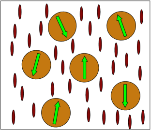
Figure 1: (Color online) Schematic illustration of ferroelectric nanoparticles suspended in a liquid crystal. The electrostatic dipole moments of the nanoparticles have a distribution of orientations.

Although the work of Ref. lopatina09 demonstrates an important physical mechanism, we must acknowledge that it has one mathematical limitation: Like all Landau theories, it involves an expansion of the free energy in powers of the order parameters. This expansion is valid when the order parameters are small, but it breaks down when they become large. In particular, the theory allows the order parameters to become larger than 1, which is clearly impossible. For ferroelectric nanoparticles in a liquid crystal, the nanoparticle order parameter is not necessarily small, even near the isotropic-nematic transition.

The purpose of the current paper is to generalize the previous theory by eliminating the assumption that the order parameters are small. For this generalization, we now use a Maier-Saupe-type theory instead of a Landau theory. We still consider the same physical concept of coupled orientational order parameters for the liquid crystals and the nanoparticles, and we still use the same energy of interaction between them. However, we now use a more general expression for the entropy, not a power series, which enforces the constraint that the order parameters cannot become larger than 1. This change allows us to avoid the potential mathematical inconsistency of Landau theory.

Like our previous calculation, the work presented here shows that doping liquid crystals with ferroelectric nanoparticles enhances the isotropic-nematic transition temperature. In the limit of weak coupling between the nanoparticles and the liquid crystal, the Maier-Saupe-type theory exactly reduces to the Landau theory. However, in the case of strong coupling, the new theory predicts a smaller but still substantial enhancement. Rough estimates suggest that the experimental system is in the limit of strong coupling, so it is important to use this modified theory. Furthermore, the work presented here also predicts the Kerr effect as a function of applied electric field. In the limit of low electric field, the Maier-Saupe-type theory exactly reduces to the Landau theory. However, for larger field, the nanoparticle order saturates and the enhanced Kerr effect is cut off.

The plan of this paper is as follows. In Sec. II we present the formalism of Maier-Saupe theory, with interacting orientational distributions for liquid-crystal molecules and nanoparticles. In Sec. III we apply this formalism to calculate the isotropic-nematic transition temperature, and determine the enhancement due to nanoparticles. In Sec. IV we use the same formalism to calculate the Kerr effect of induced orientational order under an applied electric field, and investigate how this effect depends on the magnitude of the field. Finally, in Sec. V we discuss the main conclusions of this study.

II Overview of Maier-Saupe Theory

In this section we introduce the free energy for a system of liquid-crystal molecules with ferroelectric nanoparticles. To construct the free energy, we use the fundamental equation of mean-field theory,

$$F=\langle H\rangle+k_{\mathrm{B}}T\langle\ln\varrho\rangle,$$ (1)

where the first term is the energy, the second term is the entropic contribution to the free energy, and the averages are taken over the single-particle distribution function $\varrho$. Hence, the first step is to define the distribution functions for liquid-crystal molecules and nanoparticles.

Liquid-crystal molecules are rod-shaped objects, with each molecule characterized by the direction of its long axis $\mathbf{m}$. In the nematic phase, these axes are preferentially oriented along the average director $\mathbf{n}$. Because the individual molecules are equally likely to point along $+\mathbf{n}$ or $-\mathbf{n}$, the single-molecule distribution function can be written as

$$\varrho_{\mathrm{LC}}(\theta)=\frac{\exp({U_{\mathrm{LC}}P_{2}(\cos\theta))}}{\int_{-1}^{1}d(\cos\theta)\exp({U_{\mathrm{LC}}P_{2}(\cos\theta))}},$$ (2)

where $\theta$ is the angle between the molecular orientation $\mathbf{m}$ and the average director $\mathbf{n}$, and $P_{2}$ is the second Legendre polynomial. The parameter $U_{\mathrm{LC}}$ is a variational parameter, which acts as an effective field on the molecular orientation. It is related to the standard nematic order parameter $S_{\mathrm{LC}}=\langle P_{2}(\cos\theta)\rangle$ by

$$S_{\mathrm{LC}}=\frac{\int_{-1}^{1}d(\cos\theta)P_{2}(\cos\theta)\exp({U_{\mathrm{LC}}P_{2}(\cos\theta))}}{\int_{-1}^{1}d(\cos\theta)\exp({U_{\mathrm{LC}}P_{2}(\cos\theta))}}$$ (3)

Note that $U_{\mathrm{LC}}$ ranges from 0 to $\infty$, while $S_{\mathrm{LC}}$ ranges from 0 to 1.

We can now calculate the free energy of a pure liquid-crystal system. Maier-Saupe theory assumes that the interaction energy between neighboring molecules $i$ and $j$ is proportional to $-(\mathbf{m}_{i}\cdot\mathbf{m}_{j})^{2}$. With the assumed distribution function, the average interaction energy becomes

$$F_{\mathrm{energetic}}^{\mathrm{LC}}=\langle H\rangle=-\frac{1}{3}JN_{\mathrm{LC}}S_{\mathrm{LC}}^{2},$$ (4)

where $N_{\mathrm{LC}}$ is the number of liquid-crystal molecules in the system, and $J$ is an energetic parameter proportional to the interaction strength and the number of neighbors per molecule. Furthermore, the entropic contribution to the free energy can be written as

$$F_{\mathrm{entropic}}^{\mathrm{LC}} = k_{\mathrm{B}}TN_{\mathrm{LC}}\langle\ln\varrho_{\mathrm{LC}}\rangle$$

$$= k_{\mathrm{B}}TN_{\mathrm{LC}}\Bigl{[}U_{\mathrm{LC}}S_{\mathrm{LC}}$$

$$-\ln\left[\textstyle\int_{-1}^{1}d(\cos\theta)\exp(U_{\mathrm{LC}}P_{2}(\cos\theta))\right]\Bigr{]}.$$

By combining these pieces, we obtain the total free energy of the liquid crystal,

$$\frac{F}{N_{\mathrm{LC}}k_{\mathrm{B}}T} = -\frac{J}{3k_{\mathrm{B}}T}S_{\mathrm{LC}}^{2}+U_{\mathrm{LC}}S_{\mathrm{LC}}$$

$$-\ln\left[\textstyle\int_{-1}^{1}d(\cos\theta)\exp(U_{\mathrm{LC}}P_{2}(\cos\theta))\right]$$

The free energy of Eq. (II) is a function of the temperature $T$ and the variational parameter $U_{\mathrm{LC}}$, with $S_{\mathrm{LC}}$ defined implicitly as a function of $U_{\mathrm{LC}}$ through Eq. (3). By minimizing the free energy over $U_{\mathrm{LC}}$ for varying temperature, we can find the liquid crystal has a first-order transition from the isotropic phase with $U_{\mathrm{LC}}=S_{\mathrm{LC}}=0$ to the nematic phase with

$$U_{\mathrm{LC}}=1.95,\quad S_{\mathrm{LC}}=0.429.$$ (7)

The numerical solution for the transition temperature in this pure liquid crystal is

$$T_{\mathrm{NI}}=0.147\frac{J}{k_{\mathrm{B}}}.$$ (8)

Also, we can find an analytic solution for the limit of supercooling,

$$T^{*}=\frac{2J}{15k_{\mathrm{B}}}=0.133\frac{J}{k_{\mathrm{B}}}.$$ (9)

From experiments we know $T^{*}$ and $T_{\mathrm{NI}}$ for any particular liquid-crystal material, so we can use Eq. (8) or (9) to determine $J$ for that material,

$$J=6.81k_{\mathrm{B}}T_{\mathrm{NI}}.$$ (10)

Once we add nanoparticles to the system, we get another distribution function for the orientations of the nanoparticle dipole moments. By symmetry, we expect that this distribution should be aligned along the same axis $\mathbf{n}$ as the liquid-crystal distribution. However, the magnitude of the order may be different. Hence, we can write the nanoparticle distribution function as

$$\varrho_{\mathrm{NP}}(\theta)=\frac{\exp({U_{\mathrm{NP}}P_{2}(\cos\theta))}}{\int_{-1}^{1}d(\cos\theta)\exp({U_{\mathrm{NP}}P_{2}(\cos\theta))}},$$ (11)

where $U_{\mathrm{NP}}$ is a variational parameter for the nanoparticles. The orientational order parameter $S_{\mathrm{NP}}$ of the nanoparticles can be defined by analogy with the liquid-crystal order parameter as

$$S_{\mathrm{NP}}=\frac{\int_{-1}^{1}d(\cos\theta)P_{2}(\cos\theta)\exp({U_{\mathrm{NP}}P_{2}(\cos\theta))}}{\int_{-1}^{1}d(\cos\theta)\exp({U_{\mathrm{NP}}P_{2}(\cos\theta))}}.$$ (12)

Just as in the liquid-crystal case, note that $U_{\mathrm{NP}}$ ranges from 0 to $\infty$, while $S_{\mathrm{NP}}$ ranges from 0 to 1.

As we discussed in our previous paper lopatina09 , the ferroelectric nanoparticles create static electric fields, which interact with the dielectric anisotropy of the liquid crystal. By averaging the interaction energy over the distribution functions $\varrho_{\mathrm{LC}}$ and $\varrho_{\mathrm{NP}}$, we obtain

$$F_{\mathrm{interaction}}=-K_{\mathrm{NP}}N_{\mathrm{NP}}S_{\mathrm{LC}}S_{\mathrm{NP}}.$$ (13)

In this expression, $N_{\mathrm{NP}}$ is the number of nanoparticles in the system, and $K_{\mathrm{NP}}$ is an energetic parameter representing the strength of the interaction. For an unscreened electrostatic interaction, we derived

$$K_{\mathrm{NP}}=\frac{\varepsilon_{0}\Delta\varepsilon p^{2}}{180\pi(\varepsilon_{0}\varepsilon)^{2}R^{3}}=\frac{4\pi\varepsilon_{0}\Delta\varepsilon P^{2}R^{3}}{405(\varepsilon_{0}\varepsilon)^{2}}.$$ (14)

where $p$, $P$, and $R$ are dipole moment, polarization, and radius of a nanoparticle, and $\varepsilon$ and $\Delta\varepsilon$ are the dielectric constant and dielectric anisotropy of the bulk liquid crystal. If the interaction is screened by counterions, then $K_{\mathrm{NP}}$ is somewhat reduced, but it is still substantial as long as the Debye screening length is greater than the nanoparticle radius. Hence, orientational order of the liquid-crystal molecules tends to favor orientational order of the nanoparticles, and vice versa.

Whenever there is an aligning effect, there must be an entropic cost. By analogy with the entropic term for liquid-crystal molecules, the entropic penalty for aligning the nanoparticles is

$$F_{\mathrm{entropic}}^{NP} = k_{\mathrm{B}}TN_{\mathrm{NP}}\langle\ln\varrho_{\mathrm{NP}}\rangle$$

$$= k_{\mathrm{B}}TN_{\mathrm{NP}}\Bigl{[}U_{\mathrm{NP}}S_{\mathrm{NP}}$$

$$-\ln\left[\textstyle\int_{-1}^{1}d(\cos\theta)\exp(U_{\mathrm{NP}}P_{2}(\cos\theta))\right]\Bigr{]}.$$

The total free energy for liquid-crystal molecules and nanoparticles is now the combination of Eqs. (II), (13), and (II),

$$\frac{F}{N_{\mathrm{LC}}k_{\mathrm{B}}T} = -\frac{J}{3k_{\mathrm{B}}T}S_{\mathrm{LC}}^{2}-\frac{\nu K_{\mathrm{NP}}}{k_{\mathrm{B}}T}S_{\mathrm{LC}}S_{\mathrm{NP}}$$

$$+U_{\mathrm{LC}}S_{\mathrm{LC}}+\nu U_{\mathrm{NP}}S_{\mathrm{NP}}$$

$$-\ln\left[\textstyle\int_{-1}^{1}d(\cos\theta)\exp(U_{\mathrm{LC}}P_{2}(\cos\theta))\right]$$

$$-\nu\ln\left[\textstyle\int_{-1}^{1}d(\cos\theta)\exp(U_{\mathrm{NP}}P_{2}(\cos\theta))\right].$$

Note that we have normalized this free energy by the number of liquid-crystal molecules, not by the number of nanoparticles. For that reason, all the nanoparticle terms in Eq. (II) contain a factor of $\nu=N_{\mathrm{NP}}/N_{\mathrm{LC}}$, the ratio of the number of nanoparticles to the total number of liquid-crystal molecules.

To summarize, we have derived the free energy for the system of ferroelectric nanoparticles suspended in a liquid crystal. The first term represents the aligning energy favoring orientational order of the liquid crystal, while the second term describes the mutual aligning interaction between nanoparticle order and liquid-crystal order. The last terms are entropic terms that give the free-energy penalty for any liquid-crystal or nanoparticle order. The free energy is a function of two variational parameters, $U_{\mathrm{LC}}$ and $U_{\mathrm{NP}}$, and we formulate our problem as minimization over those quantities. Once we find them, we can calculate the order parameters $S_{\mathrm{LC}}$ and $S_{\mathrm{NP}}$ using Eqs. (3) and (12).

III Transition Temperature

Experiments show a substantial increase in the isotropic-nematic transition temperature for liquid crystals doped with ferroelectric nanoparticles. In order to understand this phenomenon and predict how to enhance it further, we investigate the isotropic-nematic transition using the free energy of Eq. (II).

Two distinct limiting cases of this transition are possible. If the nanoparticle order is small, then all of the integrals in Eq. (II) can be expanded in Taylor series for small $U_{\mathrm{LC}}$ and $U_{\mathrm{NP}}$. The expressions for the order parameters $S_{\mathrm{LC}}$ and $S_{\mathrm{NP}}$ from Eqs. (3) and Eq. (12) can also be expanded in power series in $U_{\mathrm{LC}}$ and $U_{\mathrm{NP}}$. Hence, the free energy can be expressed as a series in $U_{\mathrm{LC}}$ and $U_{\mathrm{NP}}$, or equivalently as a series in $S_{\mathrm{LC}}$ and $S_{\mathrm{NP}}$. After some algebraic transformations, we obtain

$$\frac{F}{N_{\mathrm{LC}}k_{\mathrm{B}}T} = \mathrm{const}+\left(\frac{5}{2}-\frac{J}{3k_{\mathrm{B}}T}\right)S_{\mathrm{LC}}^{2}+\frac{5}{2}\nu S_{\mathrm{NP}}^{2}$$ (17)

$$-\frac{\nu K_{\mathrm{NP}}}{k_{\mathrm{B}}T}S_{\mathrm{NP}}S_{\mathrm{LC}}+\dots.$$

This expression is exactly the Landau free energy as a series in the order parameters, as discussed in our earlier paper lopatina09 . To find the isotropic-nematic transition, we first minimize over $S_{\mathrm{NP}}$ to obtain

$$S_{\mathrm{NP}}=\frac{K_{\mathrm{NP}}}{5k_{\mathrm{B}}T}S_{\mathrm{LC}}.$$ (18)

We then substitute this value into the free energy series to obtain

$$\frac{F}{N_{\mathrm{LC}}k_{\mathrm{B}}T}=\mathrm{const}+\left(\frac{5}{2}-\frac{J}{3k_{\mathrm{B}}T}-\frac{\nu K_{\mathrm{NP}}^{2}}{10(k_{\mathrm{B}}T)^{2}}\right)S_{\mathrm{LC}}^{2}+\dots.$$ (19)

The change in the coefficient of $S_{\mathrm{LC}}^{2}$ shows that the isotropic-nematic transition temperature is shifted upward by

$$\Delta T_{\mathrm{NI}}=\frac{\nu K_{\mathrm{NP}}^{2}}{25k_{\mathrm{B}}^{2}T_{\mathrm{NI}}}$$ (20a)

In the notation of the previous paper, this shift can be written as

$$\Delta T_{\mathrm{NI}}=\frac{\pi\phi_{\mathrm{NP}}R^{3}}{3T_{\mathrm{NI}}\rho_{\mathrm{LC}}}\left(\frac{2\Delta\varepsilon P^{2}}{675k_{\mathrm{B}}\varepsilon_{0}\varepsilon^{2}}\right)^{2},$$ (20b)

where $\rho_{\mathrm{LC}}$ is the number of liquid-crystal molecules per unit volume and $\phi_{\mathrm{NP}}=\frac{4}{3}\pi R^{3}\rho_{\mathrm{LC}}\nu$ is the volume fraction of nanoparticles.

Note that the power-series approximation works well as long as the energetic parameter $K_{\mathrm{NP}}$ is small compared with $5k_{\mathrm{B}}T$. In that case the nanoparticle order parameter $S_{\mathrm{NP}}$ is small compared with $S_{\mathrm{LC}}$, which is approximately 0.429 just below the isotropic-nematic transition. However, the approximation breaks down if $K_{\mathrm{NP}}$ becomes large compared with $5k_{\mathrm{B}}T$, so that $S_{\mathrm{NP}}$ is large compared with $S_{\mathrm{LC}}$. In the latter case, the prediction for $S_{\mathrm{NP}}$ would be greater than 0.429 on the nematic side of the transition. It might even be greater than 1, which would be unphysical. This unphysical prediction arises because the power-series expansion cannot take account of the saturation of the order parameters at low temperatures. Hence, for large $K_{\mathrm{NP}}$ we must consider a different limiting case.

In the limit of large $K_{\mathrm{NP}}$, the nanoparticle order is large; i.e. the variational parameter $U_{\mathrm{NP}}$ approaches infinity and the order parameter $S_{\mathrm{NP}}$ approaches 1. In that case we can approximate Eq. (12) to obtain

$$S_{\mathrm{NP}}=1-\frac{1}{U_{\mathrm{NP}}}.$$ (21)

We can then put this approximation into the free energy of Eq. (II), expand the nanoparticle entropic integral for large $U_{\mathrm{NP}}$, and minimize the resulting free energy over $U_{\mathrm{NP}}$. This calculation gives

$$U_{\mathrm{NP}} = \frac{K_{\mathrm{NP}}}{k_{\mathrm{B}}T}S_{\mathrm{LC}},$$ (22a)

$$S_{\mathrm{NP}} = 1-\frac{k_{\mathrm{B}}T}{K_{\mathrm{NP}}S_{\mathrm{LC}}}.$$ (22b)

Note that this calculation is self-consistent, showing large nanoparticle order when $K_{\mathrm{NP}}\gg k_{\mathrm{B}}T$. Using Eqs. (22), we obtain the approximate free energy of the nematic phase

$$\frac{F}{N_{\mathrm{LC}}k_{\mathrm{B}}T} = -\frac{J}{3k_{\mathrm{B}}T}S_{\mathrm{LC}}^{2}+U_{\mathrm{LC}}S_{\mathrm{LC}}$$

$$-\ln\left[\textstyle\int_{-1}^{1}d(\cos\theta)\exp(U_{\mathrm{LC}}P_{2}(\cos\theta))\right]$$

$$-\frac{\nu K_{\mathrm{NP}}}{k_{\mathrm{B}}T}S_{\mathrm{LC}}+\nu\ln\left(\frac{3K_{\mathrm{NP}}S_{\mathrm{LC}}}{2k_{\mathrm{B}}T}\right).$$

This free energy is equivalent to the classical Maier-Saupe free energy of Eq. (II), except for the last two terms, which represent the energy and entropy of well-ordered nanoparticles interacting with the liquid crystal. These terms are proportional to the nanoparticle concentration $\nu=N_{\mathrm{NP}}/N_{\mathrm{LC}}$, which is small. These terms shift the nematic free energy, and hence shift the isotropic-nematic transition temperature. To find the value of the shift, we must minimize the free energy.

To minimize the free energy, we use perturbation theory. For this calculation, we define the parameters

$$U_{\mathrm{LC}} = U_{\mathrm{LC}}^{0}+\Delta U_{\mathrm{LC}},$$ (24a)

$$T_{\mathrm{NI}} = T_{\mathrm{NI}}^{0}+\Delta T_{\mathrm{NI}},$$ (24b)

where $U_{\mathrm{LC}}^{0}$ and $T_{\mathrm{NI}}^{0}$ are the known results from the classical Maier-Saupe free energy, given in Eqs. (7) and (8), and $\Delta U_{\mathrm{LC}}$ and $\Delta T_{\mathrm{NI}}$ are perturbations due to addition of ferroelectric nanoparticles. For low nanoparticle concentrations, these perturbations should both be of order $\nu$. We now expand the free energy to lowest order in these pertubations, minimize over $\Delta U_{\mathrm{LC}}$, and solve for $\Delta T_{\mathrm{NI}}$ such that the isotropic and nematic free energies are equal. The resulting shift in the transition temperature is

$$\Delta T_{\mathrm{NI}}=1.03\frac{\nu K_{\mathrm{NP}}}{k_{\mathrm{B}}}=1.03\frac{\phi_{\mathrm{NP}}\Delta\varepsilon P^{2}}{135k_{\mathrm{B}}\rho_{\mathrm{LC}}\varepsilon_{0}\varepsilon^{2}}.$$ (25)

Comparing Eqs. (20) and (25), we can see that there are two regimes for the shift in the transition temperature. For small interaction $K_{\mathrm{NP}}$ (i.e. the Landau regime), the shift $\Delta T_{\mathrm{NI}}$ increases as $K_{\mathrm{NP}}^{2}$, but for large $K_{\mathrm{NP}}$, it increases more slowly as $K_{\mathrm{NP}}$. In both cases it is proportional to the nanoparticle concentration $\nu$. Equivalently, if we work at fixed nanoparticle volume fraction $\phi_{\mathrm{NP}}$, our theory predicts that $\Delta T_{\mathrm{NI}}$ will increase with the nanoparticle material polarization $P^{4}$ and radius $R^{3}$ in the weak-interaction regime, but it will only increase as $P^{2}$ and will be independent of $R$ in the strong-interaction regime. (It will be independent of $R$ as long as the particles are small enough so that they do not distort the liquid-crystal alignment.)

Our predictions for $\Delta T_{\mathrm{NI}}$ can be compared with the previous predictions of Li et al. li06 . They calculated that $\Delta T_{\mathrm{NI}}$ should increase as the volume fraction $\phi_{\mathrm{NP}}$ and as the polarization $P^{2}$, and should be independent of the radius $R$. These predictions for the scaling agree with our predictions for the strong-interaction regime (although not for the weak-interaction regime). We believe that this agreement is just a coincidence, because the theories are quite different. One way to see the difference is through the dependence on dielectric anisotropy $\Delta\varepsilon$: they predict that $\Delta T_{\mathrm{NI}}$ should scale as $(\Delta\varepsilon)^{2}$, but we calculate that it should scale linearly with $\Delta\varepsilon$ in the strong-interaction regime. This difference arises because their model considers one liquid-crystal molecule interacting through the dielectric anisotropy $\Delta\varepsilon$ with one nanoparticle, which then interacts through $\Delta\varepsilon$ with another liquid-crystal molecule, thus giving an effective liquid-crystal interaction proportional to $(\Delta\varepsilon)^{2}$. By comparison, in the strong-interaction regime our model considers the direct influence of well-ordered nanoparticles on the liquid crystal, and hence has only one power of $\Delta\varepsilon$.

For a numerical estimate, we use typical experimental values of the parameters $\phi_{\mathrm{NP}}=0.5\%$, $P=0.26$ Cm^-2, $R=35$ nm, $\rho_{\mathrm{LC}}=2.4\times 10^{27}$ m^-3, $k_{\mathrm{B}}=1.38\times 10^{-23}$ JK^-1, $\epsilon_{0}=8.85\times 10^{-12}$ C²N^-1m^-2, and $\Delta\epsilon\approx\epsilon\approx 10$. Those parameters imply $\nu=1\times 10^{-8}$, $K_{\mathrm{NP}}=1\times 10^{-15}$ J, and hence $K_{\mathrm{NP}}/(k_{\mathrm{B}}T)=2\times 10^{5}$, so the system is definitely in the strong-interaction regime. Our prediction for the shift in transition temperature is then

$$\Delta T_{\mathrm{NI}}\approx 1\text{ K}.$$ (26)

This value is consistent with the order of magnitude that is observed in experiments. Note that in this prediction we are using the bulk polarization of the ferroelectric material BaTiO₃, which is $P=0.26$ Cm^-2. In this respect, our current estimate is different from our previous paper lopatina09 , where we assumed $P=0.04$ Cm^-2 because of an understanding that the bulk polarization is reduced by surface effects in nanoparticles. The issue of estimating the polarization of nanoparticles is subtle, as discussed in Ref. shelestiuk11 .

As a final point about the phase diagram, we should mention that the model defined by the free energy (II) can exhibit one additional phase, between isotropic and nematic, which occurs if the parameter $K_{\mathrm{NP}}$ is sufficiently large. In this intermediate phase, the nanoparticles have substantial orientational order (with $S_{\mathrm{NP}}$ comparable to the Maier-Saupe order parameter of 0.429), but the liquid crystal has only very slight orientational order (with $S_{\mathrm{LC}}$ of order $\nu K_{\mathrm{NP}}/(k_{\mathrm{B}}T)$). For that reason, we might call it a “semi-nematic” phase. It is a perturbation on the pure liquid crystal’s isotropic phase, not on the nematic phase. The semi-nematic phase is probably an artifact of the mean-field theory used here. It can only exist because the very slight order of the liquid crystal mediates an aligning interaction between the nanoparticles. This slight orientational order is unlikely to persist when one includes fluctuations in the liquid crystal.

IV Kerr effect

Apart from the phase diagram, another important issue is the response of a liquid crystal to an applied electric field. In the isotropic phase, an applied field $E$ induces orientational order proportional to $E^{2}$, known as the Kerr effect. In most pure liquid crystals, the Kerr effect is quite small, and can only be observed for very large fields. However, in our previous paper, we predicted that ferroelectric nanoparticles can enhance the Kerr effect by several orders of magnitude. We would like to assess how this prediction is modified by the Maier-Saupe theory presented here.

In the presence of an electric field, ferroelectric nanoparticles will have polar order along the field; i.e. the orientational distribution function will no longer have a symmetry between the directions $+\mathbf{n}$ and $-\mathbf{n}$. Hence, we must change the nanoparticle distribution of Eq. (11) to

$$\varrho_{\mathrm{NP}}(\theta)=\frac{e^{U^{\mathrm{NP}}_{1}P_{1}(\cos\theta)+U^{\mathrm{NP}}_{2}P_{2}(\cos\theta)}}{\int_{-1}^{1}d(\cos\theta)e^{U^{\mathrm{NP}}_{1}P_{1}(\cos\theta)+U^{\mathrm{NP}}_{2}P_{2}(\cos\theta)}}.$$ (27)

Here, $U^{\mathrm{NP}}_{1}$ and $U^{\mathrm{NP}}_{2}$ are two variational parameters, which act as effective fields on the polar and nematic order of the nanoparticle distribution function, as described by the Legendre polynomials $P_{1}(\cos\theta))$ and $P_{2}(\cos\theta))$, respectively. They generate polar and nematic order parameters, defined as

$$M_{\mathrm{NP}} = \frac{\int_{-1}^{1}d(\cos\theta)P_{1}(\cos\theta)e^{U^{\mathrm{NP}}_{1}P_{1}(\cos\theta)+U^{\mathrm{NP}}_{2}P_{2}(\cos\theta)}}{\int_{-1}^{1}d(\cos\theta)e^{U^{\mathrm{NP}}_{1}P_{1}(\cos\theta)+U^{\mathrm{NP}}_{2}P_{2}(\cos\theta)}},$$

(28a)

$$S_{\mathrm{NP}} = \frac{\int_{-1}^{1}d(\cos\theta)P_{2}(\cos\theta)e^{U^{\mathrm{NP}}_{1}P_{1}(\cos\theta)+U^{\mathrm{NP}}_{2}P_{2}(\cos\theta)}}{\int_{-1}^{1}d(\cos\theta)e^{U^{\mathrm{NP}}_{1}P_{1}(\cos\theta)+U^{\mathrm{NP}}_{2}P_{2}(\cos\theta)}}.$$

We still assume that the liquid-crystal distribution function is purely nematic, not polar, as given by Eq. (2).

The applied electric field $E$ adds two contributions to the energy of the system,

$$F_{\mathrm{energetic}}^{\mathrm{field}}=-\frac{\varepsilon_{0}\Delta\varepsilon}{3\rho_{\mathrm{LC}}}E^{2}S_{\mathrm{LC}}N_{\mathrm{LC}}-pEM_{\mathrm{NP}}N_{\mathrm{NP}}.$$ (29)

Here, the first term is the interaction of the field with the dielectric anisotropy of the liquid crystal, and the second term is the interaction with the dipole moments of the nanoparticles. With these energetic terms, together with the entropy of the distribution function, the free energy becomes

$$\frac{F}{N_{\mathrm{LC}}k_{\mathrm{B}}T}=-\frac{J}{3k_{\mathrm{B}}T}S_{\mathrm{LC}}^{2}-\frac{\nu K_{\mathrm{NP}}}{k_{\mathrm{B}}T}S_{\mathrm{LC}}S_{\mathrm{NP}}$$

$$\qquad-\frac{\varepsilon_{0}\Delta\varepsilon E^{2}}{3k_{\mathrm{B}}T\rho_{\mathrm{LC}}}S_{\mathrm{LC}}-\frac{\nu pE}{k_{\mathrm{B}}T}M_{\mathrm{NP}}$$

$$\qquad+U_{\mathrm{LC}}S_{\mathrm{LC}}+\nu U^{\mathrm{NP}}_{1}M_{\mathrm{NP}}+\nu U^{\mathrm{NP}}_{2}S_{\mathrm{NP}}$$ (30)

$$\qquad-\ln\left[\textstyle\int_{-1}^{1}d(\cos\theta)e^{U_{\mathrm{LC}}P_{2}(\cos\theta)}\right]$$

$$\qquad-\nu\ln\left[\textstyle\int_{-1}^{1}d(\cos\theta)e^{U^{\mathrm{NP}}_{1}P_{1}(\cos\theta)+U^{\mathrm{NP}}_{2}P_{2}(\cos\theta)}\right].$$

The next step is to minimize this free energy over all three variational parameters $U_{\mathrm{LC}}$, $U^{\mathrm{NP}}_{1}$, and $U^{\mathrm{NP}}_{2}$. For this minimization, there are four distinct regimes of electric field, as indicated in Fig. 2.

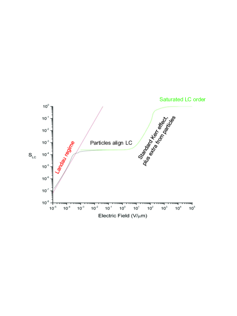
Figure 2: (Color online) Four regimes of the Kerr effect, derived from a numerical minimization of Eq. (30) with typical experimental parameters. A log-log scale is used to show all the regimes on a single plot.

(a) If the field is sufficiently small, $E\lesssim k_{\mathrm{B}}T/p$, it induces only slight order in the liquid-crystal and nanoparticle distributions. In that case, we can expand the free energy as a power series in all the variational parameters. This expansion is exactly the Landau theory presented in our previous paper lopatina09 . We can then minimize the free energy over all the variational parameters to obtain

$$S_{\mathrm{LC}}=\frac{E^{2}}{15k_{\mathrm{B}}(T-T^{*}_{\mathrm{doped}})}\left(\frac{\varepsilon_{0}\Delta\varepsilon}{\rho_{\mathrm{LC}}}+\frac{\nu K_{\mathrm{NP}}p^{2}}{5(k_{\mathrm{B}}T)^{2}}\right),$$ (31)

where $T^{*}_{\mathrm{doped}}=T^{*}+\Delta T_{\mathrm{NI}}$ is the limit of supercooling of the nanoparticle-doped liquid crystal, combining Eqs. (9) and (20). In this expression, the first term is the conventional Kerr effect without nanoparticles, and the second term is an additional contribution due to the aligning effect of the nanoparticles. Note that both terms are proportional to $E^{2}$. With the numerical estimates presented above, the second term is several orders of magnitude larger than the first, and hence the nanoparticles greatly increase the Kerr effect in this regime.

(b) For larger field, in the regime $k_{\mathrm{B}}T/p\lesssim E\lesssim[\nu K_{\mathrm{NP}}\rho_{\mathrm{LC}}/(\varepsilon_{0}\Delta\varepsilon)]^{1/2}$, the nanoparticle order parameters $M_{\mathrm{NP}}$ and $S_{\mathrm{NP}}$ saturate near the maximum value of 1. In that case, we can no longer expand the free energy as a power series in the nanoparticle parameter, but we can still expand it in the liquid-crystal parameter. Minimizing the free energy then gives

$$S_{\mathrm{LC}}=\frac{1}{15k_{\mathrm{B}}(T-T^{*})}\left(\frac{\varepsilon_{0}\Delta\varepsilon E^{2}}{\rho_{\mathrm{LC}}}+3\nu K_{\mathrm{NP}}\right).$$ (32)

Once again, the first term is the conventional Kerr effect without nanoparticles, and the second term is the additional contribution from the nanoparticles, but now the second term is independent of electric field. The second term is still much larger than the first, and hence the Kerr effect is approximately constant with respect to field in this regime.

(c) For even larger field, $[\nu K_{\mathrm{NP}}\rho_{\mathrm{LC}}/(\varepsilon_{0}\Delta\varepsilon)]^{1/2}\lesssim E\lesssim[k_{\mathrm{B}}(T-T^{*})\rho_{\mathrm{LC}}/(\varepsilon_{0}\Delta\varepsilon)]^{1/2}$, the order parameter $S_{\mathrm{LC}}$ is still given by Eq. (32), but now the first term becomes larger than the second. In this regime, $S_{\mathrm{LC}}$ again increases as $E^{2}$. It is similar to the conventional liquid-crystal Kerr effect, but with an extra constant contribution from the nanoparticles.

(d) For the largest field, $[k_{\mathrm{B}}(T-T^{*})\rho_{\mathrm{LC}}/(\varepsilon_{0}\Delta\varepsilon)]^{1/2}\lesssim E$, the order parameter $S_{\mathrm{LC}}$ saturates at the maximum value of 1.

To get a full picture of the behavior through all these regimes, we minimize the free energy of Eq. (30) numerically, using the typical experimental parameters listed at the end of Sec. III. The results of this calculation are shown by the black line in Fig. 2. By comparison, the red line shows the limiting case of regime (a), and the green line shows the approximation for regimes (b-d). We see that the numerical solution overlaps the limiting cases and connects them.

Note that the low-field regime (a) is the regime where Landau theory is valid, and it is where the nanoparticles give the greatest enhancement of the conventional Kerr effect. However, this regime will be difficult to observe in experiments, because the induced order parameter $S_{\mathrm{LC}}$ is so small, on the order of $10^{-4}$. Typical optical experiments can only detect a birefringence corresponding to $S_{\mathrm{LC}}$ on the order of $10^{-2}$, which does not occur until regime (c), which is closer to the conventional Kerr effect.

V Conclusions

In our previous paper lopatina09 , we developed a Landau theory for the statistical mechanics of ferroelectric nanoparticles suspended in liquid crystals. This theory differs from other models by considering the orientational distribution function of the nanoparticles as well the liquid crystal. It shows a coupling between the nanoparticle order and the liquid crystal order, which leads to an increase in the isotropic-nematic transition temperature and in the Kerr effect. In the current paper, we consider the same physical concept, but we improve the mathematical treatment by using a Maier-Saupe-type theory. This theory reduces to the previous Landau theory in the limit of weak interactions (for the isotropic-nematic transition) or weak electric fields (for the Kerr effect). However, it changes the results in the opposite limit, when the order parameters begin to saturate. For that reason, the new theory should make more accurate predictions for experiments.

In general, the concept of coupled orientational distribution functions should be useful for many other systems beside ferroelectric nanoparticles in liquid crystals. For example, it applies to any type of nonspherical colloidal particles, such as carbon nanotubes, in a liquid-crystal solvent. It also applies to two distinct species of nonspherical colloids suspended in an isotropic solvent, which could have a coupled ordering transition. Such systems would provide further opportunities to investigate the theory presented here.

- (1) P. Poulin, H. Stark, T. C. Lubensky, and D. A. Weitz, Science 275, 1770 (1997).
- (2) Y. D. Gu and N. L. Abbott, Phys. Rev. Lett. 85, 4719 (2000).
- (3) H. Stark, Phys. Rep. 351, 387 (2001).
- (4) M. Yada, J. Yamamoto, and H. Yokoyama, Phys. Rev. Lett. 92, 185501 (2004).
- (5) I. I. Smalyukh, O. D. Lavrentovich, A. N. Kuzmin, A. V. Kachynski, and P. N. Prasad, Phys. Rev. Lett. 95, 157801 (2005).
- (6) I. Musevic, M. Skarabot, U. Tkalec, M. Ravnik, and S. Zumer, Science 313, 954 (2006).
- (7) Y. Reznikov, O. Buchnev, O. Tereshchenko, V. Reshetnyak, A. Glushchenko, and J. West, Appl. Phys. Lett. 82, 1917 (2003).
- (8) E. Ouskova, O. Buchnev, V. Reshetnyak, Y. Reznikov, and H. Kresse, Liq. Cryst. 30, 1235 (2003).
- (9) V. Reshetnyak, Mol. Cryst. Liq. Cryst. 421, 219 (2004).
- (10) O. Buchnev, E. Ouskova, Y. Reznikov, V. Reshetnyak, H. Kresse, and A. Grabar, Mol. Cryst. Liq. Cryst. 422, 47 (2004).
- (11) A. Glushchenko, C. I. Cheon, J. West, F. Li, E. Buyuktanir, Y. Reznikov, and A. Buchnev, Mol. Cryst. Liq. Cryst. 453, 227 (2006).
- (12) V. Y. Reshetnyak, S. M. Shelestiuk, and T. J. Sluckin, Mol. Cryst. Liq. Cryst. 454, 201 (2006).
- (13) F. Li, O. Buchnev, C. I. Cheon, A. Glushchenko, V. Reshetnyak, Y. Reznikov, T. J. Sluckin, and J. L. West, Phys. Rev. Lett. 97, 147801 (2006); Phys. Rev. Lett. 99, 219901(E) (2007).
- (14) O. Buchnev, A. Dyadyusha, M. Kaczmarek, V. Reshetnyak, and Y. Reznikov, J. Opt. Soc. Am. B 24, 1512 (2007).
- (15) S. M. Shelestiuk, V. Y. Reshetnyak, and T. J. Sluckin, Phys. Rev. E 83, 041705 (2011).
- (16) M. S. S. Pereira, A. A. Canabarro, I. N. de Oliveira, M. L. Lyra, and L. V. Mirantsev, Eur. Phys. J. E 31, 81 (2010).
- (17) L. M. Lopatina and J. V. Selinger, Phys. Rev. Lett. 102, 197802 (2009).