The effect of a scanning flat fold mirror on a CMB B-mode experiment

Abstract

We investigate the possibility of using a flat-fold beam steering mirror for a CMB B-mode experiment. An aluminium flat-fold mirror is found to add $\sim$0.075% polarization, which varies in a scan synchronous way. Time-domain simulations of a realistic scanning pattern are performed, and the effect on the power-spectrum illustrated and a possible method of correction applied.

I Introduction

The prevailing $\Lambda$CDM cosmological model has been very successful in explaining many observations of the universe. However, inflation - exponential expansion within the first $\sim 10^{-35}$ s - has many uncertain details; indeed it lacks strong confirmation. Inflationary models predict a background of gravity waves Starobinsky, (1982); Starobinskii, (1983); Rubakov et al., (1982); Grishchuk, (1974); Abbott and Wise, (1984) which produce a curl-like, or “B-mode” pattern of polarization on the cosmic microwave background (CMB) on scales greater than $1^{\circ}$, which cannot be produced by density perturbations Kamionkowski et al., (1997); Zaldarriaga and Seljak, (1997). The amplitude of this signal is characterized by the tensor-to-scalar ratio, $r$, which is constrained by current measurements of the temperature power spectrum and temperature-polarization cross-correlation to a value $r<0.20$ Komatsu et al., (2010). To put tight constraints on inflationary models Bock et al., (2006) we need to detect the primordial B-mode signal, or constrain it for $r<0.01$. This requires measurement of polarization fluctuations at the level of 10 nK.

To measure this signal level is challenging, and good control of systematics is required Hu et al., (2003). A number of ground-based (QUIET Samtleben and for the QUIET collaboration, (2008), PolarBear Lee et al., (2008)), balloon-based (EBEX Grainger et al., (2008), Spider Crill et al., (2008)) and satellite-based (Planck Mandolesi et al., (2010); Lamarre et al., (2003)) experiments have been, or are close to being, fielded with the raw sensitivity to detect the B-mode signal if it is present at a reasonable $r$. These experiments are all designed to have low, and stable, instrumental polarization (IP), and often include a modulation strategy to assist with reducing systematics and mitigating against $1/f$ noise. The majority of these experiments hold their optics stationary with respect to the receiver, and scan the cryostat and optics together; a notable exception being the Tenerife experiment Davies et al., (1996). Scanning the cryostat places requirements on the stability with respect to accelerations and tilts. Although cryogenic receivers have been demonstrated that are stable at different tilt angles Grainger et al., (2010), the sensitivity to accelerations has not been demonstrated. A system can be imagined, however, which combines a stationary receiver with a fold mirror. Besides the simplification of the cryogenic requirements, the large reduction in the mass of moving components would make the design of the steerable mount much simpler.

We investigate such a system in this paper. In Section II we describe the system, and review the production of polarization from reflections. In Section III we describe a fiducal scan strategy and simulation pipeline. Results from this pipeline are then presented and discussed, along with other potential problems in Section IV.

II Method

For this investigation, we consider a horn fed receiver and compact range antenna (CRA), placed in a groundscreen, nominally observing the horizon. The output beam of the CRA is then steered to the sky with a single, flat, fold mirror. Although the flat mirror would be large; $\sim 4\times 4$ m, such a system can be considered. The flat mirror is then tipped and tilted such that the beam of the telescope moves across the sky to allow observations.

Off-normal reflections, as caused by this folding, induce a polarization. The effect is well known and is the principle behind, for example, the “pile-of-plates polarizer”. The Fresnel equations give the reflection coefficients for incident angle $\theta_{i}$ and transmission angle $\theta_{t}$ for an incident wave with E-field parallel to the boundary, $R_{\parallel}$ and $R_{\perp}$:

$$R_{\parallel}=\left(\frac{\tan^{2}(\theta_{i}-\theta_{t})}{\tan^{2}(\theta_{i}+\theta_{t})}\right)$$ (1)

and

$$R_{\perp}=\left(\frac{\sin^{2}(\theta_{i}-\theta_{t})}{\sin^{2}(\theta_{i}+\theta_{t})}\right)$$ (2)

For a metal plate, we use the relation for the complex index of refraction,

$$(n+i\kappa)^{2}=\epsilon^{\prime}+i\epsilon^{\prime\prime}$$ (3)

For a general dielectric, the conductivity $\sigma$ is given by $\sigma=\omega\epsilon^{\prime\prime}\epsilon_{0}$ where $\omega=2\pi f$ and $f$ is the radiation frequency. For a good conductor, we can assume $\epsilon^{\prime}\ll\epsilon^{\prime\prime}$, and so

$$n^{2}=\frac{\sigma}{2\omega\epsilon_{0}}$$ (4)

Plugging this into Snell’s law allows calculation of $R_{\parallel}$ and $R_{\perp}$. For a pure aluminium plate, $1/\sigma=\rho=28.2\times 10^{-9}$ $\Omega{\rm m}$, we find $R_{\parallel}=0.9970$ and $R_{\perp}=0.9985$. Thus an unpolarized input reflected with $\theta_{i}=45$ would have an overall polarization of $0.075\%$ This ignores the phase-delay from the reflections, which elliptically polarizes the reflected beam, producing both circular polarization and rotating the plane of polarization. Using a Drude-Lorentz model to calculate $n$ and $\kappa$ for aluminium at 90GHzUng and Sheng, (2007), we calculate that the plane of polarization is rotated by an additional $\sim 10^{-9}$ degrees when the phase delay is included. Ignoring this is then valid as this is a much smaller than the effect from differential reflection ($\sim 0.2^{\circ}$). The reflection is a total power to polarization conversion ($T\to Q,U$); in the context of a CMB polarization measurement the total power is 2.7 K, and so the induced polarized signal is then $\sim$200 $\mu{\rm K}$, higher than even the EE polarization spectrum. However, the signal is changing consistently with the scan, and so is varying on different scales from the CMB signals of interest and so could, in principle, be removed. In the next section, we describe the pipeline with which we investigate the effect on CMB reconstruction and $C_{\ell}$ estimation.

We note in passing that it is possible to construct a two mirror system that provides a fold with no net polarization. Consider a beam travelling along the $x$ axis. The first mirror, mounted at 45^∘ to the $yz$ plane, then reflects the beam so it is travelling along the $y$ axis, and the second, mounted at 45^∘ to the $xy$ plane, reflects that beam along the $z$. As the reflection axes have switched, both input $E_{x}$ and $E_{y}$ receive an attenuating factor of $R_{\parallel}R_{\perp}$. Any net polarization is then due to differences between the conductivity of the mirrors. If the two mirrors are fixed relative to each other, and allowed to rotate about the $x$ axis, the beam can be steered. A second set of mirrors, in a similar configuration, can be added to allow full beam steering around the sky. This is illustrated in figure 1.

Figure 1: A pair of flat-fold mirrors with no net polarization.

III Scan strategy and pipeline

We simulate observations with the following four step pipeline. Firstly, time ordered data (TOD) is simulated with 100Hz sampling for four 3-hour observation periods, corresponding to a day of observations, and the sky location (RA, Dec), telescope pointing direction (az, el), and observed $E_{x}^{2}$ and $E_{y}^{2}$ recorded. The input CMB maps were produced by simulating a power spectrum with CAMB Lewis et al., (2000), and producing a realization with the Healpix Górski et al., (2005) synfast routine. This input all-sky map was also convolved with a Gaussian beam with FWHM of 5.5 arcmin. Parameters used in the simulation are listed in Table 1. Note that we include the monopole in this simulation, with a temperature of 2.7 K and so $E_{x}^{2}\sim E_{y}^{2}\sim=1.3$ K.

It is generally desirable for ground-based and suborbital experiments to scan the sky at constant elevation to minimize the effect of variable airmass. We follow this and consider the proposed Clover scan strategy, the optimization of which is fully described elsewhere North and Johnson, . The strategy is to perform azimuthal scans at fixed elevation (nominally $45^{\circ}$) as the chosen sky patch rises for around 1 hour, continually adjusting the azimuthal center to achieve as circular a patch as possible. Once the patch has risen sufficiently through the scan, the elevation is increased, nominally to $\sim 60^{\circ}$, and the patch continues to rise for another 3 hours. The same strategy is used as the patch sets, giving four distinct data streams for a single patch during a 8-12-hour observation period.

The second step in the pipeline is to take the pointing from the TOD data, determine the angle of the flat folding mirror, rotate the observed $E_{x}^{2}$ and $E_{y}^{2}$ to align with the plane of the mirror, apply the calculated $R_{\parallel}$ and $R_{\perp}$, and then rotate back. The TOD is then naively binned to produce T, Q and U maps, following the map-making scheme outlined in Brown et al., (2009), and then written out as a Healpix format FITS files. We make maps at $N_{\rm side}=512$ so that the multipole range $\ell\sim 100$ to $1000$ is retrievable, and avoid holes in the maps by simulating a five pixel focal plane. The pixel angular positions from boresight are listed in Table 1.

Finally, the angular power spectrum (APS) coefficients $C_{\ell}$ are estimated using the anafast Healpix routine. We apply a circular mask of radius $10^{\circ}$ with a simple cosine-squared taper of width $2^{\circ}$ at the edge.

Table 1: Simulation parameters. Detector positions are given in (az, el) in the telescope frame.

Parameter	Value
Telescope location	Atacama desert
Patch centre	9h00m,-44∘00’
Patch radius	10∘
Azimuthal scan speed	0.5 deg/s
Nominal elevations	45, 60 deg
Observing frequency	90 GHz
Data rate	100 Hz
Resitivity of aluminium	$28.2\times 10^{-9}$ $\Omega{\rm m}$
Input r	0.1
Detector 1 position	(0,0) arcmin
Detector 2 position	(14.8, 14.8) arcmin
Detector 3 position	(29.6, 29.6) arcmin
Detector 4 position	(36.9, 7.4) arcmin
Detector 5 position	(51.7, 22.1) arcmin

III.1 Determination of angles

Figure 2: Fiducial geometry considered for calculating the relevant angles. Top left: the telescope beam from the dewar (direction ${\bf a}$) to the sky (${\bf b}$), directed at the azimuthal polar coordinates ($\theta_{e},\phi$). Bottom left: the angle $\alpha$ through which the beam is reflected by the mirror. Right: $E_{x}$ and $E_{y}$, the two polarization vectors on the sky.

In order to determine the effect for a mirror at an arbitrary orientation, two angles are required; the angle of incidence, $\theta_{i}$ and the angle, $\beta$, between the mirror and the horizon as seen by the incident photons. Consider the the flat fold mirror to be at the origin, and the unit vector a points to the dewar, and b points to the position on the sky being observed. This is is illustrated in figure 2. $\alpha$ is the angle between a and b. In polar coordinates, ${\bf a}=(1,90^{\circ},180^{\circ})$ and ${\bf b}=(1,\theta_{e},\phi)$ where $90-\theta_{e}$ and $\phi$ are the the elevation and azimuth of the sky location. Converting into Cartesian coordinates, we have ${\bf a}=(-1,0,0)$ and ${\bf b}=(\sin\theta_{e}\cos\phi,\sin\theta_{e}\sin\phi,\cos\theta_{e})$. To determine $\alpha$, we take the dot-product of a and b and get

$${\bf a}.{\bf b}=\cos\alpha=-\sin\theta_{e}\cos\phi$$ (5)

As the angles of incidence and reflection, $\theta_{i}$ and $\theta_{r}$ are equal, we have

$$\theta_{i}=1/2\alpha=1/2\arccos(-\sin\theta_{e}\cos\phi))$$ (6)

We define $E_{x}$ to be parallel to the horizon, and $E_{y}$ to be “upwards” towards the zenith. We require the angle $\beta$ by which $E_{x}$ and $E_{y}$ need to be rotated (around the line of sight) so that the rotated $E_{x}$ is parallel to the mirror. We define ${\bf c}$, a unit vector that points in the same direction as $E_{x}$, so, in polar, coordinates, $c=(1,90^{\circ},\phi+90^{\circ})$. ${\bf a}\wedge{\bf b}$ is parallel to the mirror. By taking the dot product of ${\bf a}\wedge{\bf b}$ with ${\bf c}$, we can determine the angle $\beta$ as

$$({\bf a}\wedge{\bf b}).{\bf c}=|({\bf a}\wedge{\bf b})||{\bf c}|\cos\beta.$$ (7)

After some algebra,

$$r=\arccos(\cos^{2}\phi).$$ (8)

Thus we have the angle of incidence, $\theta_{i}$, required for the calculation above, and we have the angle, $\beta$, so that the $R_{\parallel}$ and $R_{\perp}$ factors can be applied to the rotated $E_{x}$ and $E_{y}$.

IV Results and discussion

IV.1 Simulation Results

We use CAMB to simulate a sky, observe it with our scanning strategy code, and follow the pipeline through to calculate power spectra. Firstly we test our pipeline by ignoring the effect of the fold mirror; resultant APS are shown in figure 3. In the region of interest ($\ell\sim$100–1000) the output spectra match the input spectra well for TT and EE. The spectra from the masked pipeline maps for TT and EE are slightly supressed for larger $\ell$; 5% at at $\ell\sim 900$ when compared to the spectra made from the full sky maps. However, as the spectra from the masked full sky maps are also supressed, we conclude that this is due to the effect of the partial sky mask and fairly naive apodization procedure. Similarly, the BB spectra from the masked map is higher than the all-sky map, but as the pipeline BB spectra agrees with the masked all-sky map BB spectra, we conclude that it is the mask rather than the map-making procedure which is increasing the BB power. Although this level of analysis is not sufficient for a full B-mode experiment, this level of analysis is sufficient for investigating the effect of the flat-fold mirror.

We then apply the effect of a flat fold mirror in the pipeline, using the resistivity of aluminium of $28.2\times 10^{-9}$ $\Omega{\rm m}$, and observations at 90GHz. A section of the time stream is shown in figure 4, both the input and output $E_{x}^{2}$ and the azimuth of the observed sky location. The correlation between induced polarization with observed sky azimuth is clear.

The induced polarization is big, and so it is reasonable to remove it without requiring the entire data set. By applying the reverse of the observing algorthim, we can determine a “pre-mirror” $E_{x}$ and $E_{y}$ for a given mirror resitivity. We use $\Sigma(E_{x}^{2}-E_{y}^{2})$, summed over the day of observation for a particular pixel, as a measure of the amount of polarization, and minimize it by varying the resistivity, using the Nelder-Mead simplex direct search Lagarias et al., (1998), implemented in Matlab. This time-line can then be re-inserted into the pipeline, maps made and spectra computed. The resultant APS are shown in figure 3. We see that in the range $\ell\sim$ 100–1000, the TT, EE and BB spectra all match the pipeline output as before. In order to show problems more clearly, we also plot the difference between the spectra produced from the maps with and without the flat fold mirror. These are shown against $\ell$ in figure 5. We find that the TT and EE spectra are reconstructed well, with less than 1% difference between $\ell$ of 250 and 900. The BB spectra shows both fluctuation of $\sim 1\%$ and an overall offset of 2.5% over the same $\ell$ range.

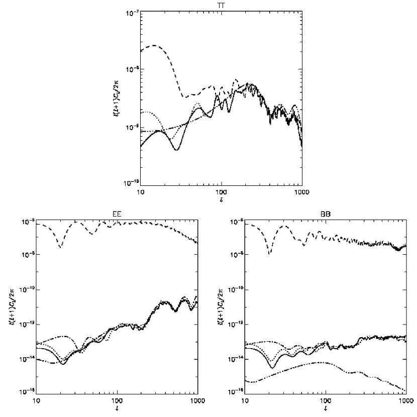
Figure 3: TT, EE, and BB spectra from various maps. dash-dot-dot-dot line is the input spectra, as simulated by CAMB. Dotted line is the all sky map, masked with the same mask used for the observed patches. solid is after our pipeline, but with no mirror. dashed is the spectra after having been observed with a flat fold mirror. dot-dash is the spectra after observed, but with the fitting algorthim (described in the text) applied.

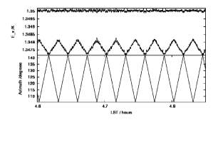
Figure 4: Upper plot: time stream of the input and observed $E_{x}$ for a noiseless simulation, with a $28.2\times 10^{-9}\Omega{\rm m}$ fold mirror. Lower plot: time stream of the telescope azimuth.

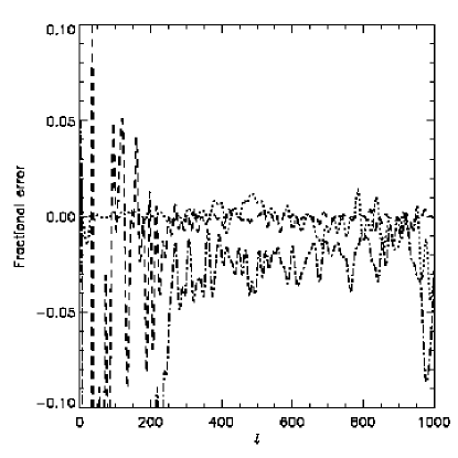
Figure 5: Fractional errors for the TT (dotted), EE (dashed) and BB (dot-dash) spectra. Calculated as the difference between the no-mirror case and the fitted mirror case, divided by the no-mirror case.

IV.2 Noise

The shortest required observing time, for a generalized CMB experiment, would be achieved using a photon noise limited telescope at a good site. For a instrument such as Clover, situated in the Atacama desert, the system NET is 175$\mu$K $\sqrt{\rm s}$. With a 100Hz data stream, this noise level overwhelms the induced polarization signal from T $\to$ Q,U mixing. However, simple binning by a factor of ten is sufficient to see the induced polarization signal in the presence of white noise. If we add white noise at the level of 175 $\mu$K $\sqrt{\rm s}$, with an $\rho=28.2\times 10^{-9}$ $\Omega{\rm m}$, the best fitting resistivity returned with this procedure is $28.8\times 10^{-9}$ $\Omega{\rm m}$.

Detector $1/f$ noise is assumed to be unimportant, assuming a detector-based modulation strategy is implemented (e.g. using a rotating or stepped half-wave plate such as EBEX, or a fast detector switching such as QUIET). Atmospheric $1/f$ total power variations contributes strongly however as the effect of the reflection is a total power to polarization conversion. Thus the atmospheric $1/f$ becomes a polarization $1/f$ term which does not get removed by any modulation strategy. A straightforward differencing strategy, for example differencing successive samples during azimuthal scanning, or differencing two adjacent detectors, to remove this varying atmospheric contribution is likely to be the most efficient method, but would reduce the effective observing time by a factor of two.

IV.3 Temperature variations

The resistivity of aluminium varies with temperature, and so the induced polarization will vary with temperature. Given a resistivity at room temperature of $\rho_{0}=28.2\times 10^{-9}\Omega{\rm m}$, the difference between the two polarization reflection coefficients is 0.075%. We introduce a temperature coefficient of resistance, $\rho_{T}$, of $3.8\times 10^{-3}{\rm K}^{-1}$, with $\rho=\rho_{0}(1+\rho_{T}\Delta T)$. Varying the temperature by 20^∘C gives a difference of 0.078% between the two polarization reflection coefficients, meaning that the T $\to$ Q,U mixing varies by $\sim 7$%. For a reasonably large flat fold mirror – in this case the flat is $\sim 2$m diameter – the temperature variation is likely to be on the timescale of hours, driven largely by the ambient temperature variations. Such variations should be removable by fitting the resistivity to the data over different timescales on a pixel-by-pixel basis. We note that, apart from the pixel on the optical axis, each pixel will see a section of the mirror whose location varies in a predictable way with azimuth (and elevation) and so fitting with respect to mirror position might also be required. In this case, the error on the fit can be reduced by fitting multiple pixel data simulatiously to produce a mirror resistivity map.

IV.4 Oxide growth

The polarizing effect of the fold mirror comes from its resistivity. As such, effects that alter the resistivity alter the polarizing effect. Aluminium grows an oxide layer very quickly, which then hydrates. The hydrated aluminium oxide can then be degraded chemically, or by physical damage to the surface. Such a surface is thin (5-15 nm) and so does not change the resistivity by a large amount. It is not unreasonable to assume that there will be changes to the surface during an extended observing campaign, both with oxide thickness and additional surface contamination. As with the temperature variation, contamination would almost certainly be localised, and so fitting resistivity with respect to mirror position would probably be required. However such changes would be expected to be slow (timescales of days or more), or at least sudden and stable, and so more data is available to fit out the effect. As a result, we expect the resistivity variation from surface oxidation and contamination to be better characterised than the temperature variation.

IV.5 Polarized foregrounds

The work so far has assumed that the light incident on the flat-fold mirror is polarized at a very low level, and that the majority of the polarized signal comes from the flat-fold mirror. This is the case when considering the CMB only, where the polarization signal has zero mean. These assumptions do not hold, however, when observing an arbitrary patch of sky, where both synchrotron and dust from the galaxy is expected to be polarized at the $\sim 1-10$% level, with a total intensity of 10–100 $\mu$K close to the Galactic Plane, but down to $\lesssim 1\mu$K at high Galactic latitudes. As such, we would recommend this method only be used in regions of known low foreground emission, where the resulting error in polarization reconstruction would be small. Over sufficiently large areas of sky the magnitude of the effect could be modelled, and in regions with relatively little large-scale variation in the foreground emission, the effect would be a constant offset, similar to an additional absolute calibration error. The areas of sky observed by most B-mode experiments are selected to meet these requirements.

In order to test this, we re-ran the simulation with some fiducial dust and synchrotron models added. After applying the same method as discussed above, the map-plane residuals are large; we see residuals of +20 to -40 $\mu$K in the Q map, in comparison with the signal level of $\pm 20\mu$K across the map. We leave fully developing this method to work in the presence of significant polarized foregrounds for future work.

V Conclusions

We have analyzed the effect of a flat-fold mirror on polarization measurements of the CMB. In the case of no foregrounds and no noise with no corrections, we find that the E and B spectra are heavily contaminated by the mixing of total power to polarization signal. However, as the CMB is expected to have a net polarization of zero, the effect can be fitted out. In the case of having a net polarization, such as in a real observation of the sky, the reconstructed maps contain significant residuals.

VI Acknowledgements

We thank Enzo Pascale and Giorgio Savini for useful discussions during this work. Some of the results in this paper have been derived using the HEALPixGórski et al., (2005).

References

- Abbott and Wise, (1984) Abbott, L. F. and Wise, M. B. (1984). Constraints on generalized inflationary cosmologies. Nuclear Physics B, 244:541–548.
- Bock et al., (2006) Bock, J., Church, S., Devlin, M., Hinshaw, G., Lange, A., Lee, A., Page, L., Partridge, B., Ruhl, J., Tegmark, M., Timbie, P., Weiss, R., Winstein, B., and Zaldarriaga, M. (2006). Task Force on Cosmic Microwave Background Research. ArXiv Astrophysics e-prints.
- Brown et al., (2009) Brown, M. L., Challinor, A., North, C. E., Johnson, B. R., O’Dea, D., and Sutton, D. (2009). Impact of modulation on CMB B-mode polarization experiments. MNRAS, 397:634–656.
- Crill et al., (2008) Crill, B. P., Ade, P. A. R., Battistelli, E. S., Benton, S., Bihary, R., Bock, J. J., Bond, J. R., Brevik, J., Bryan, S., Contaldi, C. R., Doré, O., Farhang, M., Fissel, L., Golwala, S. R., Halpern, M., Hilton, G., Holmes, W., Hristov, V. V., Irwin, K., Jones, W. C., Kuo, C. L., Lange, A. E., Lawrie, C., MacTavish, C. J., Martin, T. G., Mason, P., Montroy, T. E., Netterfield, C. B., Pascale, E., Riley, D., Ruhl, J. E., Runyan, M. C., Trangsrud, A., Tucker, C., Turner, A., Viero, M., and Wiebe, D. (2008). SPIDER: a balloon-borne large-scale CMB polarimeter. In Society of Photo-Optical Instrumentation Engineers (SPIE) Conference Series, volume 7010 of Society of Photo-Optical Instrumentation Engineers (SPIE) Conference Series.
- Davies et al., (1996) Davies, R. D., Gutierrez, C. M., Hopkins, J., Melhuish, S. J., Watson, R. A., Hoyland, R. J., Rebolo, R., Lasenby, A. N., and Hancock, S. (1996). Studies of cosmic microwave background structure at Dec.=+40 deg - I. The performance of the Tenerife experiments. MNRAS, 278:883–896.
- Górski et al., (2005) Górski, K. M., Hivon, E., Banday, A. J., Wandelt, B. D., Hansen, F. K., Reinecke, M., and Bartelmann, M. (2005). HEALPix: A Framework for High-Resolution Discretization and Fast Analysis of Data Distributed on the Sphere. ApJ, 622:759–771.
- Grainger et al., (2008) Grainger, W., Aboobaker, A. M., Ade, P., Aubin, F., Baccigalupi, C., Bissonnette, É., Borrill, J., Dobbs, M., Hanany, S., Hogen-Chin, C., Hubmayr, J., Jaffe, A., Johnson, B., Jones, T., Klein, J., Korotkov, A., Leach, S., Lee, A., Levinson, L., Limon, M., Macaluso, J., MacDermid, K., Matsumura, T., Meng, X., Miller, A., Milligan, M., Pascale, E., Polsgrove, D., Ponthieu, N., Reichborn-Kjennerud, B., Renbarger, T., Sagiv, I., Stivoli, F., Stompor, R., Tran, H., Tucker, G., Vinokurov, J., Zaldarriaga, M., and Zilic, K. (2008). EBEX: the E and B Experiment. In Society of Photo-Optical Instrumentation Engineers (SPIE) Conference Series, volume 7020 of Society of Photo-Optical Instrumentation Engineers (SPIE) Conference Series.
- Grainger et al., (2010) Grainger, W. F., Ade, P. A. R., Hargrave, P., Chase, S., Kiernan, B., and North, C. E. (2010). Thermal architecture of the Clover cryostats. In Society of Photo-Optical Instrumentation Engineers (SPIE) Conference Series, volume 7739 of Society of Photo-Optical Instrumentation Engineers (SPIE) Conference Series.
- Grishchuk, (1974) Grishchuk, L. P. (1974). Amplification of gravitational waves in an isotropic universe. Soviet Journal of Experimental and Theoretical Physics, 40:409–+.
- Hu et al., (2003) Hu, W., Hedman, M. M., and Zaldarriaga, M. (2003). Benchmark parameters for CMB polarization experiments. Phys. Rev. D, 67(4):043004–+.
- Kamionkowski et al., (1997) Kamionkowski, M., Kosowsky, A., and Stebbins, A. (1997). A Probe of Primordial Gravity Waves and Vorticity. Physical Review Letters, 78:2058–2061.
- Komatsu et al., (2010) Komatsu, E., Smith, K. M., Dunkley, J., Bennett, C. L., Gold, B., Hinshaw, G., Jarosik, N., Larson, D., Nolta, M. R., Page, L., Spergel, D. N., Halpern, M., Hill, R. S., Kogut, A., Limon, M., Meyer, S. S., Odegard, N., Tucker, G. S., Weiland, J. L., Wollack, E., and Wright, E. L. (2010). Seven-Year Wilkinson Microwave Anisotropy Probe (WMAP) Observations: Cosmological Interpretation. ArXiv e-prints.
- Lagarias et al., (1998) Lagarias, J., Reeds, J., Wright, M., and Wright, P. (1998). Convergence properties of the nelder-mead simplex method in low dimensions. SIAM Journal of Optimization, 9:112–147.
- Lamarre et al., (2003) Lamarre, J. M., Puget, J. L., Bouchet, F., Ade, P. A. R., Benoit, A., Bernard, J. P., Bock, J., de Bernardis, P., Charra, J., Couchot, F., Delabrouille, J., Efstathiou, G., Giard, M., Guyot, G., Lange, A., Maffei, B., Murphy, A., Pajot, F., Piat, M., Ristorcelli, I., Santos, D., Sudiwala, R., Sygnet, J. F., Torre, J. P., Yurchenko, V., and Yvon, D. (2003). The Planck High Frequency Instrument, a third generation CMB experiment, and a full sky submillimeter survey. New Astronomy Review, 47:1017–1024.
- Lee et al., (2008) Lee, A. T., Tran, H., Ade, P., Arnold, K., Borrill, J., Dobbs, M. A., Errard, J., Halverson, N., Holzapfel, W. L., Howard, J., Jaffe, A., Keating, B., Kermish, Z., Linder, E., Miller, N., Myers, M., Niarchou, A., Paar, H., Reichardt, C., Spieler, H., Steinbach, B., Stompor, R., Tucker, C., Quealy, E., Richards, P. L., and Zahn, O. (2008). POLARBEAR: Ultra-high Energy Physics with Measurements of CMB Polarization. In H. Kodama & K. Ioka, editor, American Institute of Physics Conference Series, volume 1040 of American Institute of Physics Conference Series, pages 66–77.
- Lewis et al., (2000) Lewis, A., Challinor, A., and Lasenby, A. (2000). Efficient computation of CMB anisotropies in closed FRW models. Astrophys. J., 538:473–476.
- Mandolesi et al., (2010) Mandolesi, N., Bersanelli, M., Butler, R. C., Artal, E., Baccigalupi, C., Balbi, A., Banday, A. J., Barreiro, R. B., Bartelmann, M., Bennett, K., Bhandari, P., Bonaldi, A., Borrill, J., Bremer, M., Burigana, C., Bowman, R. C., Cabella, P., Cantalupo, C., Cappellini, B., Courvoisier, T., Crone, G., Cuttaia, F., Danese, L., D’Arcangelo, O., Davies, R. D., Davis, R. J., De Angelis, L., de Gasperis, G., De Rosa, A., De Troia, G., de Zotti, G., Dick, J., Dickinson, C., Diego, J. M., Donzelli, S., Dörl, U., Dupac, X., Enßlin, T. A., Eriksen, H. K., Falvella, M. C., Finelli, F., Frailis, M., Franceschi, E., Gaier, T., Galeotta, S., Gasparo, F., Giardino, G., Gomez, F., Gonzalez-Nuevo, J., Górski, K. M., Gregorio, A., Gruppuso, A., Hansen, F., Hell, R., Herranz, D., Herreros, J. M., Hildebrandt, S., Hovest, W., Hoyland, R., Huffenberger, K., Janssen, M., Jaffe, T., Keihänen, E., Keskitalo, R., Kisner, T., Kurki-Suonio, H., Lähteenmäki, A., Lawrence, C. R., Leach, S. M., Leahy, J. P., Leonardi, R., Levin, S., Lilje, P. B., López-Caniego, M., Lowe, S. R., Lubin, P. M., Maino, D., Malaspina, M., Maris, M., Marti-Canales, J., Martinez-Gonzalez, E., Massardi, M., Matarrese, S., Matthai, F., Meinhold, P., Melchiorri, A., Mendes, L., Mennella, A., Morgante, G., Morigi, G., Morisset, N., Moss, A., Nash, A., Natoli, P., Nesti, R., Paine, C., Partridge, B., Pasian, F., Passvogel, T., Pearson, D., Pérez-Cuevas, L., Perrotta, F., Polenta, G., Popa, L. A., Poutanen, T., Prezeau, G., Prina, M., Rachen, J. P., Rebolo, R., Reinecke, M., Ricciardi, S., Riller, T., Rocha, G., Roddis, N., Rohlfs, R., Rubiño-Martin, J. A., Salerno, E., Sandri, M., Scott, D., Seiffert, M., Silk, J., Simonetto, A., Smoot, G. F., Sozzi, C., Sternberg, J., Stivoli, F., Stringhetti, L., Tauber, J., Terenzi, L., Tomasi, M., Tuovinen, J., Türler, M., Valenziano, L., Varis, J., Vielva, P., Villa, F., Vittorio, N., Wade, L., White, M., White, S., Wilkinson, A., Zacchei, A., and Zonca, A. (2010). Planck pre-launch status: the Planck-LFI programme. ArXiv e-prints.
- (18) North, C. and Johnson, B. Clover scan strategy, in prep. in prep.
- (19) Note1. http://healpix.jpl.nasa.gov.
- Rubakov et al., (1982) Rubakov, V. A., Sazhin, M. V., and Veryaskin, A. V. (1982). Graviton creation in the inflationary universe and the grand unification scale. Physics Letters B, 115:189–192.
- Samtleben and for the QUIET collaboration, (2008) Samtleben, D. and for the QUIET collaboration (2008). QUIET - Measuring the CMB polarization with coherent detector arrays. ArXiv e-prints.
- Starobinskii, (1983) Starobinskii, A. A. (1983). The Perturbation Spectrum Evolving from a Nonsingular Initially De-Sitter Cosmology and the Microwave Background Anisotropy. Soviet Astronomy Letters, 9:302–+.
- Starobinsky, (1982) Starobinsky, A. A. (1982). Dynamics of phase transition in the new inflationary universe scenario and generation of perturbations. Physics Letters B, 117:175–178.
- Ung and Sheng, (2007) Ung, B. and Sheng, Y. (2007). Interference of surface waves in a metallic nanoslit. Opt. Express, 15(3):1182–1190.
- Zaldarriaga and Seljak, (1997) Zaldarriaga, M. and Seljak, U. (1997). All-sky analysis of polarization in the microwave background. Phys. Rev. D, 55:1830–1840.