Rectification of motion in nonlinear media with asymmetric random drive

Abstract

We consider moving particles in media with nonlinear friction and drive them by an asymmetric dichotomic Markov process. Due to different energy dissipations, during the forward and backward stroke, we obtain a mean non-vanishing directed flow of the particles. Starting with the stationary velocity distribution, we calculate the stationary current of particles, the variance and the relative variance in dependence on the degree of nonlinearity of the friction, on the asymmetry and for different strengths of friction. In two dimensions the particle performs diffusional motion, if in addition the direction of the asymmetric drive changes stochastically.

PACS:05.40.$-$a

Keywords: Self-propelled particles, nonlinear friction, dichotomous Markovian process, diffusion

Devoted to P. Hänggi on occasion of his 60th birthday.

1 Introduction

The occurrence of directed flows of matter or single particles, in case of mean vanishing forces, is always connected with a break of symmetry in the considered medium or device. Since the pioneering work of H. Purcell [1] a lot of work has been devoted to this problem. Purcell found that simple devices require more than one degree of freedom by which they can temporally store energy sequentially in an asymmetric way. Later on, theoretical work on ratchets has elaborated the many different combinations of possible constructions between nonlinear periodic potentials, noise and forcing to obtain non-vanishing flows of particles if the averaged sum of forcing vanishes [2, 3, 4, 5, 6, 7]. It was P. Hänggi who put forward the notion of Brownian motors [3, 8, 9] to point out the possibility to find engines in the presence of a strongly fluctuating environment. Most strikingly, in many cases this noisy environment can even act as the source of energy which drives the engine (the interested reader is referred to [10] for Peter Hänggi’s extended list of publications on Brownian motors and the various different topics he has investigated).

In this paper we study particles moving in a medium with nonlinear friction [11, 12, 13, 14]. Therefore, the rate of dissipation will depend on their velocity. Achieving different values of velocity will result in a different speed of dissipation. We will drive such particles by random forces with a vanishing average. We assume a two state random telegraph signal or a dichotomous Markov process as force acting on the particle [15, 16, 17, 18]. Crucially, we will assume that this force acts asymmetrically, i.e. its two values in the two directions will be different. Such an applied asymmetric force elongates the velocity of the particle differently during the forward and backward stroke. Hence, it will dissipate the transmitted energy during both strikes differently. For this reason the particle is able to perform a directed motion even in the case if the applied drive vanishes on average.

We will assume that the random drive is a time homogeneous stochastic process. Hence, the problem becomes stationary in the long time limit and we can use tools from the theory of stationary stochastic processes. As a result we calculate the mean velocities and the variance of the velocities for the one dimensional case. In two dimensions, we add a stochastic rotation of the direction of the applied asymmetric forcing and show first numeric results for the diffusional motion of the particle.

We mention that similar problems have been discussed within the framework of vibrational dynamics by Blekhman (see e.g. [19]), who has used an alternative approach in the case of a fast periodic driving to find asymptotic velocities of gliding particles in many different situations. This approach is based on the separation of time scales and averaging over the fast time scale of the driving force. Similar techniques have also been used as approximate solutions to elaborate instabilities in driven oscillators, see e.g. the Kapiza-(Magnus)pendulum in [20]. An application to our stochastic driving is also possible, but here we rely on techniques using the stationary probability density for the particle’s velocity.

2 Nonlinear friction and asymmetric forcing

We study singular particles with unit mass $m=1$ which move in a fluid. Therein the particles experience a frictional force $f(v)$ which damps the motion. To compensate the damping, the particles are forced by additive temporal forces $\xi(t)$. We assume that this force possesses a vanishing mean and stationary correlations

$$\left\langle\xi(t)\right\rangle=0\,,~{}~{}~{}\left\langle\xi(t)\xi(t^{\prime})\right\rangle=K(t-t^{\prime})\quad.$$ (1)

Thus the velocity $v(t)$ of the particles obeys the following dynamical equation

$$\dot{v}\left(t\right)=f\left(v(t)\right)+\xi(t)\quad.$$ (2)

The time-dependent force $\xi(t)$ drives the system permanently out of (thermal) equilibrium. The velocity distribution is non-Maxwellian. We underline that there is no spatial dependence in the description (2). This typical ingredient of Brownian ratchets, namely spatially periodic gradients, is absent in our model. Thus the rectification process of (2) differs from the usual Brownian ratchet mechanism [3]. As outlined, symmetry is broken due to the asymmetric forcing realizing an asymmetric energy dissipation by the nonlinear friction.

As driving force we will consider a random telegraph signal $\xi(t)$ which is a time-homogeneous Markov process. It can take two values $\left\{A_{+},A_{-}\right\}$ with constant transition rates $\kappa_{-}/\kappa_{+}$ between the two states. $\kappa_{+}$ denotes the rate of passage from $A_{+}$ to $A_{-}$ and analogously, $\kappa_{-}$ denotes the rate of passage from $A_{-}$ to $A_{+}$. The resulting time correlation function reads

$$\langle\xi(t)\xi(s)\rangle=\frac{(A_{+}-A_{-})^{2}\kappa_{+}\kappa_{-}}{(\kappa_{+}+\kappa_{-})^{2}}\cdot e^{-(\kappa_{+}+\kappa_{-})|t-s|}\quad.$$ (3)

Particular interest will be paid to unbiased dichotomous Markov processes, i.e. processes with a vanishing mean $\left\langle\xi(t)\right\rangle=0$, which leads to

$$A_{+}\kappa_{-}+A_{-}\kappa_{+}=0\quad.$$ (4)

The condition (4) reduces the amount of independent parameters to three. We therefore introduce the following set of three independent parameters of the unbiased DMN process

$$A=|A_{-}|+|A_{+}|,~{}~{}~{}\tau=\tau_{-}+\tau_{+},$$

$$0<p=\frac{\min(|A_{-}|,|A_{+}|)}{\max(|A_{-}|,|A_{+}|)}<1,$$ (5)

where the mean waiting times $\tau_{\pm}$ for the states $A_{\pm}$ relate to the rates as $\tau_{\pm}=1/k_{\pm}$. The parameter $A$ measures the strength of the DMN process. $\tau$, the mean time of one cycle, is the characteristic time scale of the DMN. It differs from the correlation time $\tau_{C}=(\kappa_{+}+\kappa_{-})^{-1}$. The parameter $p$ will be the desired parameter controlling the asymmetry of the driving. Symmetric driving is located exactly at $p=1$. High asymmetries, i.e. when the stroke amplitudes $|A_{-}|$ and $|A_{+}|$ differ much, let $p$ tend to zero.

We can express the variance of the DMN in terms of the new parameters, resulting in

$$var\left\{\xi\right\}=\langle\xi^{2}(t)\rangle=\frac{A^{2}p}{(1+p)^{2}}\quad.$$ (6)

The variance increases with the driving amplitude $A$. This is not rather surprising. However, while looking at the variance profile for a varying asymmetry $p$, one observes, that the variance reaches its maximum when the driving is totally symmetric. On the other hand, growing asymmetry (i.e. lower values of $p$) reduce the variance. In the asymmetric limit $p\to 0$, the variance vanishes completely.

In particular we are interested in the effect of nonlinear friction. Therefore it will be convenient to introduce a model of friction that can model nonlinearity via a parameter, in order to easily control the impact of nonlinearity on the system (2). Prominent types of friction, are the so called Stokes friction ($f(v)=-\gamma_{s}v$), which is typical for small particles moving at low velocities through viscous fluids, and the “quadratic drag force” ($f(v)=-\gamma_{q}|v|v$), corresponding to situations of objects moving at relatively large velocities through fluids, a widely occurring situation in aerodynamical engineering. Another prominent type of friction is the so called Coulomb friction ($f(v)=-\gamma_{c}\frac{v}{|v|}$). This form of friction characterizes sliding frictions, the form of friction that occurs, when two surfaces slide against each other. This situation is sometimes called “dry friction”. The respective friction coefficients $\gamma_{i}$ depend specifically on the characteristics of the fluid and of the corresponding particles.

Moreover, Stokes friction is a linear friction model, while the other two models, quadratic and Coulomb friction, are nonlinear. Our model of friction $f(v)$ should be able to model more general forms of friction, but at the same time able to reproduce the mentioned three prominent models of friction as specific limit cases. An immediate candidate for such a model is apparently

$$f(v) =-\gamma|v|^{n}\mbox{sign}(v) \gamma>0,\quad n\in\mathbb{R}^{+}\quad.$$ (7)

This friction model introduces two parameters, namely the friction coefficient $\gamma$ and the friction exponent $n$, allowing to model a wide range of relevant types of friction beyond the introduced cases ($n=0,1,2$). The friction of general fluids, that are omnipresent in small scaled biological systems, may therefore be properly modeled by (7) (see e.g. [19]).

In the other limit, for $n\to\infty$, (7) reduces to

$$f_{\infty}(v)=\lim_{n\to\infty}f(v)=\begin{cases}+\infty&\text{for $v>1$},\\ 0&\text{for $\|v\|<1$},\\ -\infty&\text{for $v<-1$}.\end{cases}$$ (8)

The motion of the particle is constraint to the velocities between $-1$ and $1$, since the damping friction forces (8) approaches infinity for $|v|>1$. In the region $|v|<1$ the particle moves freely, without damping, while at the height of the barrier sites $|v|=1$, the particle gets reflected back to lower velocities. This is in some sense similar to a particle moving in a potential well, with infinite slopes of the respective walls. Note that in this case there is no dependence on any friction constant $\gamma$ anymore.

3 Stationary currents: Analytically tractable models

In general, it is impossible to obtain an exact solution of, for instance, the stationary density of a system, if an arbitrary form of noise, especially colored noise, is considered. However, the simple structure of the DMN, as a Markovian two-state process, enables us to obtain exact and explicit results in terms of stationary distributions [16, 18, 21, 22]. The stationary solution $P_{st}$ for Eq.(2) reads

$$P_{st}\left(v\right) ={N|i_{+}(v)i_{-}(v)|}$$ (9)

$$\times\exp\biggl{[}-\kappa_{+}\int^{v}i_{+}(s)ds-\kappa_{-}\int^{v}i_{-}(s)ds\biggr{]},$$

where the functions $i_{\pm}(v)$ are defined as

$$i_{\pm}(v)=\frac{1}{-\gamma|v|^{n}\textmd{sign}(v)+A_{\pm}}\quad.$$ (10)

As one can see with Eq.(2) and (7), the support of the stationary distribution is a compact interval $[v_{-},v_{+}]$, with $v_{+}=\sqrt[n]{A_{+}/\gamma}$ and $v_{-}=-\sqrt[n]{A_{-}/\gamma}$, and beyond this interval the stationary distribution has to vanishes.

In order to compute the integrals in Eq.(9), we look at the general expression $\textstyle\frac{1}{ax^{n}+C}$ , for arbitrary $a,C,x,n\in\mathbb{R}$. Notice that we can always write

$$\begin{split}\frac{1}{ax^{n}+C}=\frac{1}{C}\sum_{i=0}^{\infty}(\frac{ax^{n}}{C})^{i},\end{split}$$ (11)

as far as $\tfrac{ax^{n}}{C}<1$ holds.

Integrals of this expression can be expressed by the the standard classical (or Gaussian) hypergeometric series ${}_{2}\mathbb{F}_{1}$. In its general form, it is defined as

$${}_{2}\mathbb{F}_{1}\left[a,b,c,z\right]=\sum_{n=0}^{\infty}\frac{(a)_{n}(b)_{n}}{(c)_{n}}\frac{z^{n}}{n!},\qquad\mbox{for $a,b,c,z\in\mathbb{C}$}\quad.$$ (12)

Integration of Eq.(11) yields

$$\begin{split}\int^{z}\frac{dx}{ax^{n}+C}&=\frac{x}{C}\,_{2}\mathbb{F}_{1}\left[\frac{1}{n},1,1+\frac{1}{n},\frac{a}{C}z^{n}\right]\end{split}$$ (13)

and consequently

$$\begin{split}\int^{v}i_{\pm}(v)dv=\begin{cases}&\displaystyle{\frac{v}{A_{\pm}}}\,_{2}\mathbb{F}_{1}\left[\frac{1}{n},1,1+\frac{1}{n},-\frac{\gamma v^{n}}{A_{\pm}}\right]\,~{}~{}v>0,\\ \\ &\displaystyle{\frac{v}{A_{\pm}}}\,_{2}\mathbb{F}_{1}\left[\frac{1}{n},1,1+\frac{1}{n},\frac{\gamma(-v)^{n}}{A_{\pm}}\right]\,v<0.\\ \end{cases}\end{split}$$

Stationary moments can be computed straightforwardly. However, in general it will be difficult to give an analytic closed formula for the stationary moments. That is why we will first look at special cases and discuss the general case of arbitrary $n\in\mathbb{R}^{+}$ in the context of simulations later on.

Let us start with the dry friction limit ($n=0$), i.e.

$$\dot{v}=-\gamma\ \mbox{sign}(v)+\xi(t)\quad.$$ (14)

Notice that for the case $\gamma>max(|A_{-}|,|A_{+}|)$ no motion can occur at all, since the critical force in order to induce motion is $\pm\gamma$. In this case the stationary distribution $P_{st}^{0}$ takes the form

$$P_{st}^{0}(v)=\delta(v),$$ (15)

where the $\delta$ function denotes the Dirac distribution.

To exclude this situation, we require $\gamma<min(|A_{-}|,|A_{+}|)$. Then the critical friction force is overcome in both situations, in the state $A_{+}$ as well as in the state $A_{-}$ of the DMN $\xi(t)$.

The functions $i_{\pm}(v)$ simply become constants which results in

$$\begin{split}P_{st}^{0}(v)&=-N\begin{cases}\dfrac{\exp\biggl{[}-\dfrac{\kappa_{+}v}{-\gamma+A_{+}}-\dfrac{\kappa_{-}v}{-\gamma+A_{-}}\biggr{]}}{\left(-\gamma+A_{+}\right)\left(-\gamma+A_{-}\right)}&\,v>0,\\ \\ \dfrac{\exp\biggl{[}-\dfrac{\kappa_{+}v}{\gamma+A_{+}}-\dfrac{\kappa_{-}v}{\gamma+A_{-}}\biggr{]}}{\left(\gamma+A_{+}\right)\left(\gamma+A_{-}\right)}&\,v<0.\end{cases}\end{split}$$ (16)

The stationary distribution $P_{st}^{0}$ is an exponential function for every half line ($v>0$, $v<0$). Note that for (16) to be normalizable, the exponentials should converge to zero in the limits of infinity $\textstyle v\to\pm\infty$. Therefore it is sufficient to show, that the exponentials on every half line are decaying, which is in accordance with our assumptions $A_{+}>0$, $A_{-}<0$, $\kappa_{\pm},\gamma>0$ and $\gamma<\min(|A_{-}|,|A_{+}|)$.

If the driving is asymmetric, we get two different limits for the distribution function at the origin $v=0$, since

$$\lim_{v\to 0^{+}}P_{st}^{0}(v)=\frac{N}{\left(-\gamma+A_{+}\right)\left(-\gamma+A_{-}\right)}$$ (17)

and the left side limit yields

$$\lim_{v\to 0^{-}}P_{st}^{0}(v)=\frac{N}{\left(\gamma+A_{+}\right)\left(\gamma+A_{-}\right)}\quad.$$ (18)

Thus, the stationary distribution is discontinuous at $v=0$ in the dry friction limit ($n=0$).

For the normalization constant $N$ we get

$$N=-\frac{\gamma\kappa}{2}\quad.$$ (19)

with $\kappa=\kappa_{+}+\kappa_{-}$. The first moment, as the mean average velocity and stationary current $J=\textstyle\left\langle v\right\rangle$, gives

$$\left\langle v\right\rangle=\frac{A_{-}+A_{+}}{\kappa}\quad.$$ (20)

Hence, in the dry friction limit, the particle moves in the direction of the stronger of both strokes $A_{\pm}$. If $|A_{+}|>|A_{-}|$, the particle moves into the positive direction while in the opposite case it moves backwards. Remarkably, $\left\langle v\right\rangle$ does not explicitly depend on the (critical) friction force $\gamma$. No matter how strong the stiff friction force $\gamma$ is, as long as $\gamma<min(|A_{-}|,A_{+}|)$ is ensured, the average velocity $\left\langle v\right\rangle$ does not depend on the friction. Expressing the mean velocity (20) in terms of the three effective parameters of the driving $p,A$ and $\tau$, we obtain

$$\left\langle v\right\rangle=A\tau\frac{p(p-1)}{(p+1)^{3}}\quad,$$ (21)

where we assumed, without loss of generality, $\textstyle|A_{-}|>|A_{+}|$. Remember that we have per definition $\textstyle 0<p<1$. Thus, in this case the current is negative. For a symmetric driving ($p=1$) the velocity vanishes exactly. However, the velocity vanishes also if $\textstyle p\to 0$. That is why too much asymmetry is not a successful way to obtain the optimum speed in the dry friction limit. Therefore we expect a maximum of the mean velocity within the region $\textstyle p\in[0,1]$. This result is confirmed by the numerical simulations shown in Fig.(1).

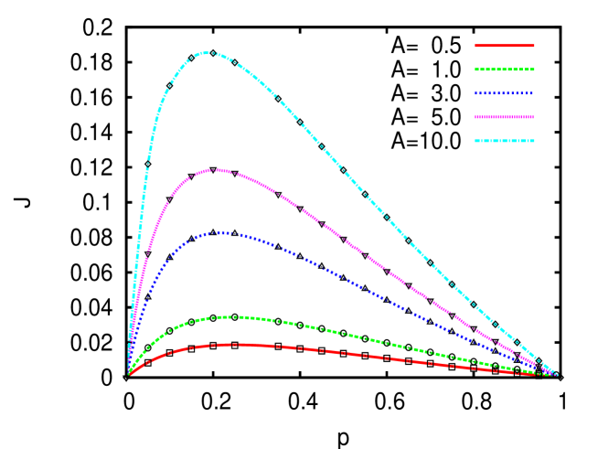
Figure 1: Case of dry friction: current versus asymmetry parameter $p$ for different stroke amplitudes $A$. The current shows a maximum for optimal asymmetry [29].

We now turn shortly to the case of Stokes friction ($n=1$ or $f(v)=-\gamma v$) and will take a look at the mean velocity. For the stationary distribution $P_{st}^{1}$ we compute

$$P_{st}^{1}(v)=N\ \lvert-\gamma v+A_{+}\rvert^{\frac{\kappa_{+}}{\gamma}-1}\ \lvert-\gamma v+A_{-}\rvert^{\frac{\kappa_{-}}{\gamma}-1}\quad.$$ (22)

To determine the first moment $J=\left\langle v\right\rangle$, we get

$$\begin{split}\left\langle v\right\rangle=&\int_{\frac{A_{-}}{\gamma}}^{\frac{A_{+}}{\gamma}}v(-\gamma v+A_{+})^{\frac{k_{+}}{\gamma}-1}(-\gamma v+A_{-})^{\frac{\kappa_{-}}{\gamma}-1}dv\\ &=\frac{c\Gamma[\frac{\kappa_{-}}{\gamma}]\Gamma[\frac{\kappa_{+}}{\gamma}]}{\Gamma[\frac{\kappa}{\gamma}+1]}\underbrace{\left(A_{+}\kappa_{-}+A_{-}\kappa_{+}\right)}_{=0}=0\quad.\end{split}$$ (23)

Thus we have obtained, that in the linear case, there can never be a current for vanishing mean forcing. The ratchet mechanism does not work for linear friction.

In the limit of $n\to\infty$, there is no current as well. Since the relation (8) holds, there is no friction forces in the interval $v\in[-1,1]$. Here $P_{st}^{\infty}(v)$ is constant. Hence, the first moment vanishes and for the second moment we get $\left\langle v^{2}\right\rangle=1/3$.

4 Stationary current: The general case

In general cases ($n\in\mathbb{R}^{+}$), the analytical treatment is difficult. Therefore we will turn to numerical measures and our primary focus will lie on the mean velocity $\left\langle v\right\rangle$ which equals the stationary current. In addition, we will look at the variance $var\left\{v\right\}$ and at the inverse relative variance

$$coh\{v\}=\frac{\left\langle v\right\rangle^{2}}{\left\langle v^{2}\right\rangle-\left\langle v\right\rangle^{2}}$$ (24)

which might serve as a measure of coherence of the transport [23]. High coherency means, that one has a low spread in the transport process compared to the unidirectional drift.

The impact of the nonlinearity parameter $n$ on the mean velocity $\left\langle v\right\rangle$ is displayed in Fig.(2) (with $n\in[0,4]$) for different realizations of the friction coefficient $\gamma$ and the driving asymmetry $p$.

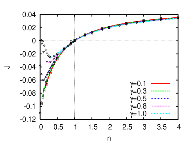
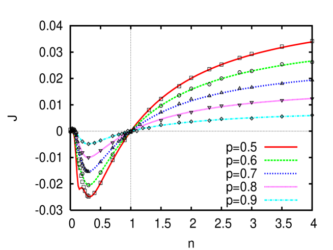
Figure 2: Current $J$ versus friction exponent $n$ for different friction coefficients $\gamma$ (top) and driving asymmetries $p$ (bottom) [29].

In all these cases we observe a single current reversal exactly at the linear friction regime $n=1$. In other words, there is no transport for linear friction. This is exactly the result we have found analytically. In particular, sublinear ($\textstyle n<1$) and superlinear ($n>1$) friction results in opposing velocity directions. While for sublinear friction, one observes a negative current, we get a positive current for the superlinear friction regime. Note that, without loss of generality, we have assumed $|A_{-}|>|A_{+}|$. In the opposite case ($|A_{+}|>|A_{-}|$), one gets the same picture with inverse sign. While the sublinear regime (dry friction regime) results in the direction of the stronger amplitude, the superlinear regime favors the opposite direction. In the dry friction limit, we observe a different behavior. If $\gamma<\max(|A_{-}|,|A_{+}|)$ holds, the current becomes a non-zero value. Otherwise the current vanishes. This is exactly what we predicted already in the analytical study of the dry friction limit $n=0$. In the superlinear case the stationary current does weakly depend on the friction. In the limit of large $n$, the current will disappear.

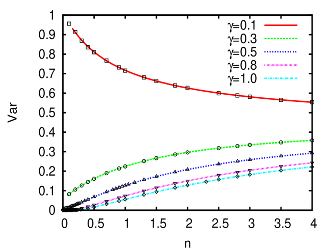
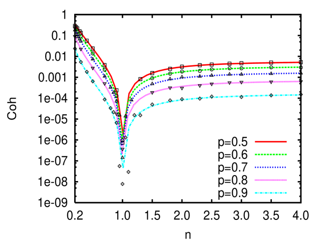
Figure 3: Variance of velocity for different friction coefficients $\gamma$ (top) and coherence (Eq.(24)) for different driving asymmetries $p$ (bottom) versus friction exponent $n$ [29].

The variance of the velocity is shown in Fig.(3). When the critical force cannot be overcome by the driving, the variance again vanishes in the dry friction limit. In this situation the variance increases with growing friction exponent $n$. In the case, where the critical force can be overcome by the driving forces, we observe a finite variance for $n=0$, which decreases with increasing friction exponent.

The coherence is presented in Fig.(3). Since the current $J$ vanishes for linear friction and at the same time the variance keeps finite, we observe that the transport coherence tends to vanish. We also see, that for superlinear friction ($n>1$), the dependency of the coherence on the exponent $n$ is very weak. $coh\{v\}$ almost does not change with varying friction exponent $n$. Whereas we observe a rather strong dependence on the exponent $n$ in the sublinear regime. In the limit $n\to 0$, the coherence increases exponentially. Thus, the dry friction regime shows much better coherence than the friction regime, which occurs in fluids.

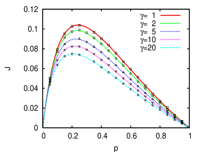
Figure 4: Current $J$ versus driving asymmetry $p$ for different friction coefficients $\gamma$ [29].

Let us now investigate the asymmetry parameter $p$. In Fig.(4) one observes in all cases a single maxima at symmetry percentages below 0.5, varying slightly for different parameter settings. In accordance with our previous considerations, the current vanishes for a symmetric driving as well as in the strongly asymmetric case. This is elucidated by the specific values of driving amplitudes $A_{\pm}$ and waiting times $\tau_{\pm}$ in this limit

$$\lim_{p\to 0}A_{-} =-A,\qquad\lim_{p\to 0}A_{+}=0,$$ (25)

$$\lim_{p\to 0}\tau_{-} =0,\qquad~{}~{}\;\;\lim_{p\to 0}\tau_{+}=\tau\quad.$$ (26)

The average waiting time $\tau_{-}$ for the state $A_{-}$ vanishes. Consequently, no negative force $A_{-}$ acts. On the other hand, no positive force acts as well, according to (25). Hence, no forces at all are acting, if $p=0$.

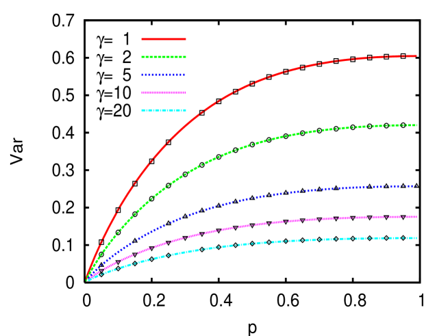
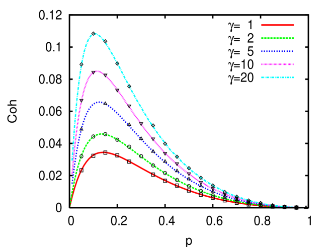
Figure 5: Variance (top) and coherence (Eq.(24);bottom) for different friction coefficients $\gamma$ versus driving asymmetry $p$ [29].

The same line of argument shows, that the variance also vanishes in the asymmetric limit. Indeed, the results confirm our ideas (Fig.(5)). Thus, starting at zero for $p=0$, the variance, in any case, increases, until it reaches its maximum for $p=1$. This can be understood in terms of the driving $\xi(t)$, which has already shown this behavior (Eq. (6)). It seems reasonable that the variance of the state variable $v$ follows qualitatively the variance of its driving.

The behavior of the coherence (Fig.(5)) shows similarities to the behavior of the current $J$. One observes a single maximum, which this time is shifted to higher asymmetries, i.e. to lower values of $p$, compared to the location of the maxima of the current. For the regarded cases, the peaks of the current are in regions where $p>0.2$ holds, while the peaks of the coherence are located below that barrier. We observe a much better localization of the maxima of the coherence, compared to those of the current.

5 Diffusion in the two dimensional case

Eventually, we present results for the two dimensional case. We assume that the asymmetric drive $\xi(t)$ acts on the particle along a certain variable direction in the two dimensional space. This direction is given by the unit vector with Cartesian coordinates

$$\vec{e}_{v}(t)={\cos\Theta(t)\choose\sin\Theta(t)}$$ (27)

and $\Theta(t)$ is the present angle between the direction of the drive and the $x$-coordinate. Along this axis, the particle changes $v(t)$ with positive and negative values according to Eq.(1) and

$$\frac{{\rm d}}{{\rm d}t}\vec{r}(t)=\vec{v}(t)\,~{}~{}\mbox{while}~{}~{}\vec{v}(t)=v(t)\cdot\vec{e}_{v}(t)\quad.$$ (28)

Additionally, a Gaussian white noise source, labeled $\eta(t)$, rotates the moving-axis of the particle. As equation for the angle $\Theta(t)$, we formulate

$$\frac{{\rm d}}{{\rm d}t}\Theta(t)=\frac{1}{v}\eta(t),$$ (29)

which assumes that the increment of the rotation angle scales with $1/v$. The noise $\eta(t)$ is defined by $\langle\eta(t)\rangle=0$ and $\langle\eta(t)\eta(t^{\prime})\rangle=2D_{\eta}\delta(t-t^{\prime})$.

For the following simulations, we fixed the friction exponent $n=3$ with $|A_{+}|>|A_{-}|$, the intensity of the noise $D_{\eta}=0.1$ and all other parameters as stated in [29].

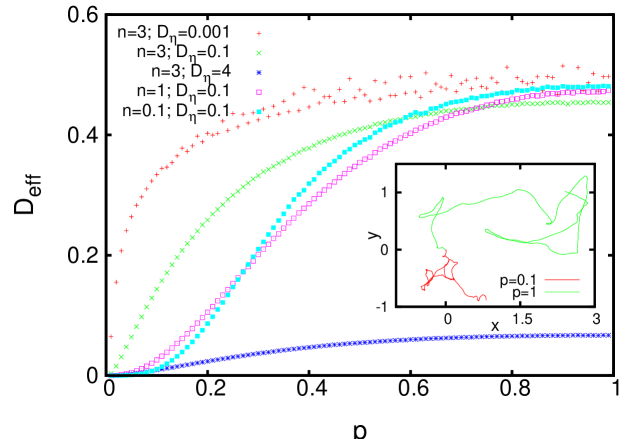
Figure 6: Diffusion coefficient of the two dimensional motion versus driving asymmetry $p$ for several $D_{\eta}$ and different friction exponents $n$; spatial trajectories for two different driving asymmetries $p$ in the inset [29].

The motion of the particle shows a diffusive behavior after a crossover. Due to the noisy rotations of the asymmetric force, no preferred direction exists. Typical trajectories are presented in the inset of Fig.(6). Simulations show that the velocity distribution densities have, for not too small $\tau$, a vanishing derivative at $v\to 0$ and possess two peaks according to the asymmetric drive. This can be expected in regard to the one dimensional case ([24] and Eq.(9)). In the two dimensional velocity space, two circles with high probabilities occur.

For large time scales, we assume $\langle(\vec{r}(t)-\vec{r}(t_{0}))^{2}\rangle=4tD_{eff}$. The resulting behavior of the diffusion coefficient (Fig.(6)) can be explained by the trajectories in the inset. They illustrate the impact of the small force $A_{-}$ which acts most of the time for $p=0.1$ and which leads to a stronger influence of the angular noise, compared to the symmetric case $p=1$.

As a possible explanation, we use the Taylor-Kubo-relation [25, 26]

$$\langle(\vec{r}(t)-\vec{r}(t_{0}))^{2}\rangle=2t\cdot\int_{0}^{\infty}C_{\vec{v}\vec{v}}(\tau)\mathrm{d}\tau\quad.$$ (30)

In simulations we have inspected that the velocity correlations $C_{\vec{v}\vec{v}}(\tau)$ increases for stronger symmetries $p$ in the driving due to an increased standard deviation of the velocities. Therefore the diffusion coefficient $D_{eff}$ is maximal for symmetric noise.

The slowly growing diffusion for small friction exponents and small driving symmetries $p$ (Fig.(6)), can be explained by the nearly vanishing velocity $v_{-}$, which mostly acts in this limit and depends on $A_{-}$. We also observe that larger noises $D_{\eta}$ lead to smaller diffusion coefficients. This behavior has already been studied in similar systems [25, 27] and is caused by a straight movement for small angular noise. The analytical treatment of the diffusion coefficient, for the one dimensional DMN process, has been recently studied for a symmetric driving [28] and corresponds to our results for $p=1$ in the limit of small noises $D_{\eta}$.

6 Conclusion and outlook

We have shown that directed motion in nonlinear media is possible, if particles are driven by an asymmetric force. The force can have external or internal origin. Small additive noise would only partially destroy the obtained effect as was seen in calculation of the stationary distribution densities [18]. In the one dimensional case, it results in a smoothing of the densities but the averaged motion will survive. Diffusion will be obtained with properties similar to the recently studied case with symmetric drive [28].

While the analytically and numerically studied one dimensional case is well understood, the behavior of particles in two dimensions remains still a challenge. Also further energetic consideration will be helpful in order to estimate the efficiency of the proposed ratchet. Future fields of interest will include also alternative two dimensional models for DMN processes and the influence of coupling forces to external obstacles or mutually to similar objects. We also see a great challenge in the consideration of different friction terms or periodically changing friction forces in order to simulate rhythmic movements in biological systems.

7 Acknowledgments

This paper was supported by DFG-Sfb 555 “Nonlinear complex processes” and by VW-Foundation “New conceptional approaches to modeling and simulating complex systems”. We acknowledge help by Jessica Strefler who has been previously involved in this study.

References

- [1] E. M. Purcell, Am. J. Phys. 45, 3 (1977).
- [2] M. Magnasco, Phys. Rev. Lett. 71, 1477 (1993).
- [3] P. Hänggi and F. Marchesoni, Rev. Mod. Phys. 81, 387 (2009).
- [4] R. D. Astumian, Science 276, 917 (1997).
- [5] P. Reimann and P. Hänggi, Appl. Phys. A 75, 169 (2002).
- [6] H. Linke, Appl. Phys. A 75, 167 (2002).
- [7] V. Anishchenko, A. Neiman, A. Astakhov, T. Vadiavasova, and L. Schimansky-Geier, Chaotic and Stochastic Processes in Dynamic Systems, Springer-Series on Synergetics (Springer Verlag, Berlin, 2002).
- [8] R. Bartussek and P. Hänggi, Phys. Bl. 51(6), 506 (1995).
- [9] R.D. Astumian, P. Hänggi, Phys. Today 55(11), 33 (2002).
- [10] www.physik.uni-augsburg.de/theo1/publikationen/html/brownian.shtml
- [11] S. Denisov, Phys. Lett. A 296, 197 (2002).
- [12] L. Schimansky-Geier, W. Ebeling and U. Erdmann, Acta Phys. Pol. B 36, 5 (2005).
- [13] B. Lindner, New J. Phys. 9, 136 (2007).
- [14] J. Strefler, W. Ebeling, E. Gudowska-Nowak and L. Schimansky-Geier, Eur. Phys. J. B 72, 597 (2009).
- [15] C. W. Gardiner, Stochastic Methods in Physics, Chemistry and Natural Sciences, Springer-Series on Synergetics (Springer, Berlin, 1990).
- [16] W. Horsthemke, R. Lefever, Noise-Induced Transitions, Springer-Series on Synergetics (Springer Verlag, Berlin, 1984).
- [17] I. Bena, Int. J. Mod. Phys. B 20, 2825 (2006).
- [18] B. Dybiec and L. Schimansky-Geier, Eur. Phys. J. B 57, 313 (2007).
- [19] I. Blekhman, Vibrational Mechanics (World Scientific Publishing, Singapore, 2000).
- [20] L. D. Landau and E. M. Lifschitz, Lehrbuch für Theoretische Physik, Band 1: Theoretische Mechanik (Akademie-Verlag, Berlin, 1990).
- [21] K. Kitahara, W. Horsthemke, R. Lefever, Y. Inaba, Prog. Theor. Phys. 64, 1233 (1980).
- [22] K. Kitahara, W. Horsthemke, R. Lefever, Phys. Lett. A 70, 377 (1979).
- [23] J. A. Freund and L. Schimansky-Geier, Phys. Rev. E 60, 1304 (1999).
- [24] J. M. Sancho, J. Math. Phys. 25, 354 (1984).
- [25] L. Haegqwist, L. Schimansky-Geier, I. Sokolov, and F. Moss, Europ. Phys. J. Special Topics 157, 33 (2008).
- [26] L. Schimansky-Geier, U. Erdmann and N. Komin, Physica A 351, 51 (2005).
- [27] A. Mikhailov, D. Meinköhn, Self-motion in physico-chemical systems far from thermal equilibrium, in Stochastic Dynamics edited by L. Schimansky-Geier, T. Pöschel, Vol. 484 of Lecture Notes in Physics, pp.334-345 (Springer, Berlin, 1997).
- [28] B. Lindner, private communication.
- [29] The default values are , meaning that, when a parameter is not specified in the plot, then its value is the default value.