Active Motion Assisted by Correlated Stochastic Torques

Abstract

The stochastic dynamics of an active particle undergoing a constant speed and additionally driven by an overall fluctuating torque is investigated. The random torque forces are expressed by a stochastic differential equation for the angular dynamics of the particle determining the orientation of motion. In addition to a constant torque, the particle is supplemented by random torques which are modeled as an Ornstein-Uhlenbeck process with given correlation time $\tau_{c}$. These nonvanishing correlations cause a persistence of the particles’ trajectories and a change of the effective spatial diffusion coefficient. We discuss the mean square displacement as a function of the correlation time and the noise intensity and detect a nonmonotonic dependence of the effective diffusion coefficient with respect to both correlation time and noise strength. A maximal diffusion behavior is obtained if the correlated angular noise straightens the curved trajectories, interrupted by small pirouettes, whereby the correlated noise amplifies a straightening of the curved trajectories caused by the constant torque.

I Introduction

Recent experimental studies evidenced that living beings, such as bacteria beta , different water fleas daphniapattern , fish fish , birds edwards and insects bazazi ; BazRom , are able to sustain a constant mean speed over large time scales. Thus, these animals do not only perform passive Brownian motion, but instead exhibit a so-called active stochastic motion SchEb98 , occurring far from equilibrium.

Such systems form a large field of recent theoretical interest MiCa01 ; schweitzer , including the influence of fluctuations. One might relate the sources of fluctuations on animal motion either in the food supply StEb09 or in the propulsive engine RoLsg11 that drives the unit or by assuming a molecular agitation imposed externally outside beta . In this approach one widely uses similarities of the animal motion and Brownian motion which Einstein and Smoluchowski independently described in a probabilistic theory einstein ; smoluchowski . Later on, Langevin encoded this theory of stochastic systems into the Newtonian notation of equations of motion langevin , which present a first formulation of a stochastic differential equation. This concept, completed by an active element describing the self-propulsion, is nowadays widely used for the description of fluctuating animal motion MiCa01 ; schweitzer ; SchEb98 ; StEb09 ; RoLsg11 . Of foremost interest are the specific effects of the random impacts on the motion.

Our focus here is on agents subjected to a torque, resulting in circular motions. This feature can be caused, for example, by an external magnetic field with profound physiological implications kanokov , or due to boundary conditions fish . The agents themselves may exhibit a preferred turning direction, either caused by asymmetries in the propulsion as occurring in the chemotaxis of sperm cells friedrich2 ; sperm2 , as a search strategy WeSr81 ; MuWe94 , or also by interaction with other agents, which leads to the emergence of swarming characteristics daphniapattern ; pavelswarm .

We start out by studying the planar motion of active particles with a constant velocity $v_{0}$ subjected to a constant torque $\Omega$. To take into account thermal or, more generally, the stochastic influence of the surrounding, we first consider an additional white Gaussian noise $\xi(t)$ driving the angle dynamics and discuss the resulting effective diffusion coefficient $D_{\text{eff}}$ lsgzigzag ; TefLow08 ; HaLsg08 ; TefLo09 . Next, we propose a more realistic model considering some persistence in the motion. Therefore, we replace the white Gaussian noise by a time-correlated Gaussian noise (colored noise), namely an Ornstein-Uhlenbeck process (OUP) $\theta(t)$ uhlenbeck ; Horsthemke_Lefever ; PH78 ; HMG84 ; Hwa89 ; JunHan_color , which implies a memory for the curvature feature. This generalization then allows applications reaching from stochastic polymer dynamics doi over spiral wave motion SenAl00 up to animal trajectories fish . This present study using a constant torque $\Omega$ can principally also be applied to a different problem, namely the control of diffusion of electron beams in drift chambers in presence of additional magnetic fields blum . We want to mention that other noise statistics, especially white Poissonian noise hanggi ; JunHan_color ; RoLsg11 , are conceivable. Their study would form an interesting future extension of the present work.

In a driven motion with a constant speed $v_{0}$ the correlations with correlation time $\tau_{c}$ generate a persistence length $l_{c}$ of the trajectory: $l_{c}=v_{0}\tau_{c}$. As will be shown below, the inclusion of correlations will hence characteristically modify the dynamics. The resulting dynamics will be quantified by the spatial diffusion coefficient $D_{\rm eff}$.

II Agents driven by white Gaussian noise

Our starting point is the equation of motion in two dimensions with a constant velocity $v_{0}$ and a random torque with the mean value $\Omega$. The dynamics for the position vector ${\vec{r}}(t)=\{x(t),y(t)\}$ derives from its velocity vector, reading

$${\rm{d\over dt}}\vec{r}(t)\,=\,v_{0}\vec{e}_{v(t)}=\,v_{0}\,\Big{(}\cos{\phi(t)},\,\sin{\phi(t)}\Big{)}\,,$$ (1)

with $\phi(t)$ denoting the orientation of the velocity vector. This orientation $\phi(t)$, if governed by a constant torque and supplemented by random fluctuations, yields a stochastic dynamics for $\phi(t)$

$${\rm{d\over dt}}{\phi}(t)\,=\,\Omega+\frac{\sqrt{2D_{\xi}}}{v_{0}}\xi(t)\,.$$ (2)

We consider the noise $\xi(t)$ to be a white Gaussian noise with the corresponding noise intensity denoted by $D_{\xi}$ and with vanishing mean. The $1/v_{0}$ in front of the random force is caused by the fact that the tangential acceleration scales as $v_{0}\dot{\phi}$. It expresses the circumstance that fast agents cannot change their direction as quickly as slower ones.

For a vanishing noise intensity the constant torque leads to circular shaped motion, whose size is dictated by their cyclotron radius $R=v_{0}/\Omega$. A non-vanishing noise intensity on the other hand induces a more erratic behavior. The mean square displacement (MSD) corresponding to this dynamics can be directly calculated by using the shifted Gaussian transition probability distribution $P(\Delta\phi,\tau)$. Then the general expression for the MSD of a particle with a constant velocity $v_{0}$, i.e.

$$\left<(\vec{r}(t)-\vec{r}_{0})^{2}\right>=2v_{0}^{2}\int_{0}^{t}(t-\tau)\left<\mathrm{cos}\left(\Delta\phi(\tau)\right)\right>\mathrm{d}\tau,$$ (3)

yields in the case of white Gaussian noise

$$\left<(\vec{r}(t)-\vec{r}_{0})^{2}\right>_{\text{white}}=2v_{0}^{2}\int_{0}^{t}(t-\tau)e^{-\frac{D_{\xi}\tau}{v_{0}^{2}}}\cos{(\Omega\tau)}\mathrm{d}\tau.$$ (4)

For small times $t$ a ballistic behavior $\propto t^{2}$ results while for large times a crossover to diffusive motion $\propto t$ takes place. The effective diffusion coefficient $D_{\text{eff}}$ in two dimensions is related to the MSD via the well-known relation:

$$D_{\text{eff}}=\lim_{t\rightarrow\infty}\frac{\langle(\vec{r}(t)-\vec{r}_{0})^{2}\rangle}{4t}\,.$$ (5)

As a consequence we integrate Eq. (4) in the limit of large times. Furthermore, we substitute a dimensionless integration variable $x=D_{\xi}v_{0}^{-2}\tau$ and obtain together with the new parameters $D_{0}=v_{0}^{4}/(2D_{\xi})$ and $\omega_{0}=\Omega v_{0}^{2}/D_{\xi}$ an expression for the effective diffusion coefficient, reading

$$D_{\text{eff}}^{\text{white}} =D_{0}\int_{0}^{\infty}e^{-x}\cos\left(\omega_{0}x\right)dx=\frac{D_{0}}{1+\omega_{0}^{2}}$$ (6)

$$=\frac{D_{\xi}}{2\left[\left(\frac{D_{\xi}}{v_{0}^{2}}\right)^{2}+\Omega^{2}\right]}.$$ (7)

Thus, we recover the result for a white Gaussian angle drive with constant torque. This finding was obtained before in Ref. lsgzigzag and has been re-addressed with Ref. TefLow08 , see for more detailed discussions HaLsg08 . Obviously, the diffusion as a function of the angular noise exhibits a maximum, with $D_{\text{eff}}=v_{0}^{2}/(4\Omega)$ at $D_{\xi}=v_{0}^{2}\Omega$, and vanishes for both $D_{\xi}=0$ and $D_{\xi}\rightarrow\infty$. This is contrasted to the behavior of the diffusion without a torque, $D_{\text{eff}}^{\Omega=0}=v_{0}^{4}/(2D_{\xi})$ othmer ; mikhailov , which diverges for $D_{\xi}\rightarrow 0$.

The explanation is as follows: for small noise intensities, agents subjected to a constant torque move in circles around a fairly quasi-stationary center, whereas in absence of a torque the propagation proceeds along almost straight lines. With noise included, both motion types perform diffusion. This leads to a reduction of the mean square displacement in case of zero torque. In contrast, agents subjected to a constant torque start to spread over the space which is expressed by the numerator in Eq. (7), which grows linearly in $D_{\xi}$. For large noise intensities $D_{\xi}$, this leads to a suppression of diffusion as accounted for in (7).

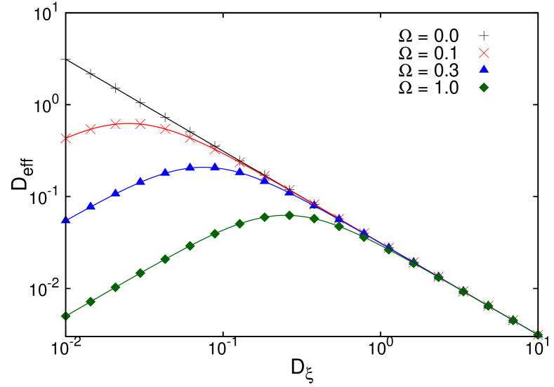
Figure 1: (Color online) Effective diffusion coefficient $D_{\text{eff}}^{\text{white}}$ versus intensity $D_{\xi}$ of the Gaussian white noise for different torque strengths $\Omega$, with the constant velocity $v_{0}=0.5$ and $D_{\xi}=0.01$ within theory, see in eq. (7).

We note that a finite torque always decreases $D_{\text{eff}}^{\text{white}}$, because the cosine-contribution in Eq. (4) suppresses the value of the integral. This difference becomes most striking for small noise intensity $D_{\xi}$. In Fig. 1 the behavior of eq. (7) is depicted as a function of $D_{\xi}$ for several $\Omega$-values.

III Agents Driven by an Ornstein-Uhlenbeck-Process

III.1 General outlines

As a physically more realistic extension of our model, we next study time-correlated noise (i.e. colored noise) for the angular drive instead of delta-correlated noise around its mean $\Omega$. Accordingly, we use an OUP as the most natural continuous-valued colored noise Horsthemke_Lefever ; PH78 ; HMG84 ; Hwa89 ; JunHan_color . Hence, our new system with the constant velocity $v_{0}$ and the torque $\Omega$ is described by the modified angle dynamics, reading

$$\dot{\phi}(t)\,=\; \Omega+\frac{1}{v_{0}}\theta(t),$$ (8)

$$\dot{\theta}(t)\,=\; -\frac{1}{\tau_{c}}\theta(t)+\sqrt{\frac{2D_{\xi}}{\tau_{c}^{n}}}\xi(t).$$ (9)

This colored noise dynamics assumes one additional auxiliary process, namely the OUP $\theta(t)$ with the correlation time $\tau_{c}$, the Gaussian white noise $\xi(t)$ and the corresponding noise intensity $D_{\xi}/\tau_{c}^{n}$.

Note that we included here a dependence of the correlation time to the power $n$ in the noise intensity implying a corresponding change in dimension for $D_{\xi}$ as $n$ changes. In doing so, several different physical features can be addressed with no need to perform additional calculations. For example, for $n=0$ the random variable $\theta(t)$ merges with the Wiener process $W(t)$ in the limit of infinite correlation times $\tau_{c}\to\infty$. In specific detail: $\dot{\theta}=\sqrt{2D_{\xi}}\xi(t)\Rightarrow\theta(t)=\sqrt{2D_{\xi}}\int^{t}\xi(t^{\prime})dt^{\prime}=\sqrt{2D_{\xi}}W(t)$. On the other hand, the case with $n=1$ delivers a variance of $\theta$, which is independent of the correlation time JunHan_color .

¿From a theoretical point of view, the case with $n=2$ is of utmost interest. The limit $\tau_{c}\rightarrow 0$ yields Gaussian white noise, i.e. $\theta(t)\rightarrow\sqrt{2D_{\xi}}\xi(t)$, and thus allows a comparison with the findings taken from Sec. II.

The corresponding $\theta$-correlation function reads in the stationary limit

$$\langle\theta(t)\theta(0)\rangle_{s}\,=\;\tau_{c}^{1-n}D_{\xi}e^{-\frac{|t|}{\tau_{c}}},$$ (10)

depicting a strong $n$-dependence of the variance, i.e. the factor in front of the exponential.

To study the angular dynamics $\phi(t)$, we use the results of Ornstein and Uhlenbeck uhlenbeck , which were later generalized by Chandrasekhar to motion in a higher dimensional space chandrasekhar . Therewith we can write the probability distribution in the stationary limit for a transition during $\tau$ from $\phi_{1}$ to $\phi_{2}$ and conditioned by $\theta_{1}$ as

$$P_{\mathrm{OUP}}(\phi_{2},\tau|\phi_{1},\theta_{1})\;=\sqrt{\frac{v_{0}^{2}}{2\pi\tau_{c}^{3-n}D(\tau)}}\\ \times\exp\left[-\frac{v_{0}^{2}\left(\phi_{2}-\phi_{1}-\Omega\tau-\theta_{1}\tau_{c}\left(1-e^{-\frac{\tau}{\tau_{c}}}\right)\right)^{2}}{2\tau_{c}^{3-n}D(\tau)}\right].$$ (11)

Here, the mean square increment of the angle holds

$$D(\tau)=D_{\xi}\left(\frac{2\tau}{\tau_{c}}-3+4e^{-\frac{\tau}{\tau_{c}}}-e^{-\frac{2\tau}{\tau_{c}}}\right).$$ (12)

This resulting Gaussian expression can be directly used to calculate the mean square displacement of our angle dynamics from Eq. (3), yielding with statioary Gaussian distributed initial values $\phi_{1}$ and $\theta_{1}$

$$\langle(\vec{r}(t)-\vec{r}_{0})^{2}\rangle_{\text{OUP}}=\;2v_{0}^{2}\int_{0}^{t}(t-\tau)e^{-\Psi(\tau)}\cos{(\Omega\tau)}\mathrm{d}\tau\,.$$ (13)

The function in the exponent reads

$$\Psi(\tau)=\;\Psi_{0}\left(\frac{\tau}{\tau_{c}}-1+e^{-\frac{\tau}{\tau_{c}}}\right).$$ (14)

wherein we define

$$\Psi_{0}\,=\,\frac{\tau_{c}^{3-n}D_{\xi}}{v_{0}^{2}}\,,$$ (15)

as a parameter which scales monotonously with $\tau_{c}$ and $D_{\xi}$ and can therefore be used to discuss the asymptotic behavior, later on.

Without constant torque ($\Omega=0$) and with $n=0$ this reproduces the result of fish2 , where the motion of fish was analyzed within a similar model. Furthermore, Eq. (13) exhibits a crossover from a ballistic behavior $\propto t^{2}$ to diffusive motion $\propto t$. This can be seen by studying the following two temporal limits

$$\lim_{t\to 0}{\rm{d\over dt}}\langle(\vec{r}(t)-\vec{r}_{0})^{2}\rangle_{\text{OUP}} =2\,v_{0}^{2}\,t\,,$$ (16)

$$\lim_{t\to\infty}{{\rm d}\over{\rm d}t}\langle(\vec{r}(t)-\vec{r}_{0})^{2}\rangle_{\text{OUP}} =2v_{0}^{2}\int_{0}^{\infty}e^{-\Psi(\tau)}\cos{(\Omega\tau)}{\rm d}\tau.$$ (17)

The right-hand side of Eq. (17) is obviously a non-vanishing constant which can be identified with the effective diffusion coefficient via Eq. (5), yielding our central finding, namely

$$D_{\text{eff}}^{\text{OUP}}=\frac{v_{0}^{2}}{2}\int_{0}^{\infty}e^{-\Psi(\tau)}\cos{(\Omega\tau)}{\rm d}\tau.$$ (18)

For further analytical discussions it will be helpful to use a dimensionless representation of Eq. (18). To this end, we substitute $x=\frac{\tau}{\tau_{c}}\Psi_{0}$ and introduce the rescaled variables

$$D_{c}=\frac{v_{0}^{4}}{2\tau_{c}^{2-n}D_{\xi}}\qquad\text{and}\qquad\omega_{c}=\frac{v_{0}^{4}\Omega}{\tau_{c}^{2-n}D_{\xi}},$$ (19)

yielding

$$D_{\text{eff}}^{\text{OUP}}=D_{c}\int_{0}^{\infty}e^{-x}e^{\Psi_{0}\left(1-e^{-x/\Psi_{0}}\right)}\cos{(\omega_{c}x)}{\rm d}x.$$ (20)

In comparison with the results for a white Gaussian angle drive [c.f. Eq. (7)] we notice different definitions of the constants $D_{c}$ and $\omega_{c}$ and an additional exponential in the integrand, namely $e^{\Psi_{0}\left(1-e^{-x/\Psi_{0}}\right)}$. The latter converges to unity for $\Psi_{0}\rightarrow 0$ and increases monotonously with $\Psi_{0}$. For $n=2$, the parameters $\omega_{c}$ and $D_{c}$ coincide with those defined in the white noise case, respectively, with $D_{0}$ and $\omega_{0}$. In this case $\Psi_{0}$ describes the deviation from the results under white noise.

Also note that the integral in Eq. (20) can be expressed in a serial expansion. Substituting first $z=\Psi_{0}\exp(-x/\Psi_{0})$ as a new variable and expanding afterwards the remaining exponential under the integral in a Taylor series, one can calculate the integral in each summand, yielding

$$D_{\text{eff}}^{\text{OUP}}=D_{c}e^{\Psi_{0}}\sum_{k=0}^{\infty}\frac{(-1)^{k}}{k!}\Psi_{0}^{k+1}\frac{\Psi_{0}+k}{(\Psi_{0}+k)^{2}+(\Psi_{0}\omega_{c})^{2}}.$$ (21)

The asymptotic behavior of the diffusion coefficient can be readily derived: For vanishingly small $\Psi_{0}$, the first item in the sum with $k=0$ dominates. Hence we obtain

$$\lim_{\Psi_{0}\to 0}D_{\text{eff}}^{\text{OUP}}\,=\,\lim_{\Psi_{0}\to 0}\frac{D_{c}}{1+\omega_{c}^{2}},$$ (22)

which in particular recovers the white noise result of eq. (7) for the case $n=2$.

The opposite asymptotics of large $\Psi_{0}$ can be inspected by looking at the original integral definition in Eq. (20), (see also fish2 ) for the case without an applied torque and $n=0$. In this limit the major contributions to the integral stem from values at the lower boundary $x\sim 0$. Upon expanding the double exponent until the second order finds

$$\lim_{\Psi_{0}\to\infty}D_{\text{eff}}^{\text{OUP}}\,\propto\lim_{\Psi_{0}\to\infty}D_{c}\sqrt{\Psi_{0}}\exp\left(-\frac{\Psi_{0}\omega_{c}^{2}}{2}\right),$$ (23)

which tends to zero much faster compared to the case without torque with $\omega_{c}=0$.

III.2 Asymptotic behavior in the absence of torque: $\Omega=0$

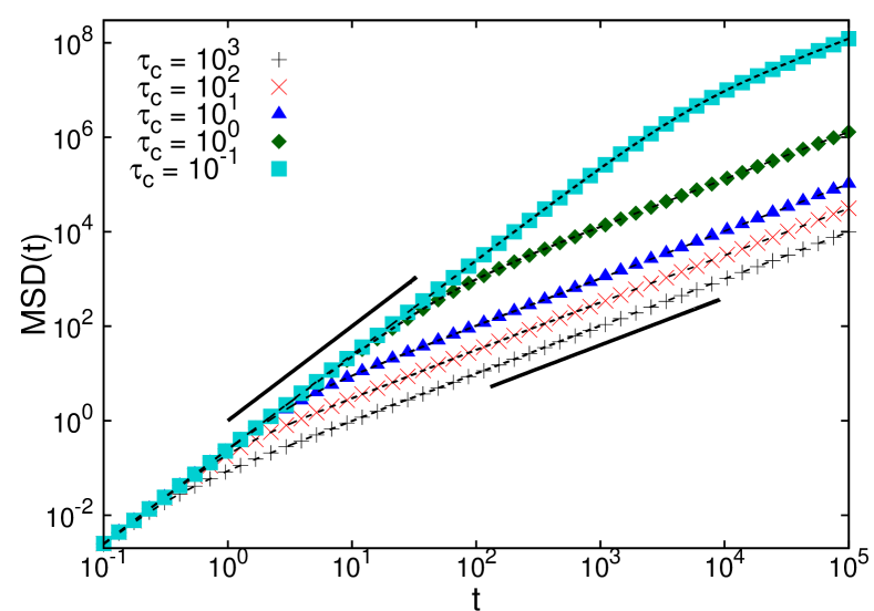
Figure 2: (Color online) Mean square displacement $\langle(\vec{r}(t)-\vec{r}_{0})^{2}\rangle$ for the dynamics given with Eqs. (8) and (9) for $\Omega=0$, $D_{\xi}=0.01$, $v_{0}=0.5$ and with $n=0$. Simulations (points) agree well with the theory (Eq. (13); dashed lines). The left bar is $\propto t^{2}$, the right bar is $\propto t$. For $\tau_{c}\gtrsim 3$, the ratio of subsequent crossover times behaves according to $t_{\text{cross}}(\tau_{c})/t_{\text{cross}}(10\tau_{c})=\sqrt{10}$, otherwise according to $t_{\text{cross}}(\tau_{c})/t_{\text{cross}}(10\tau_{c})=10^{2}$.

First we study the crossover between the ballistic and the diffusive behavior. Towards this aim we expand the two exponentials in Eq. (13). A case differentiation, due to the two corresponding exponential time dependencies, yields two parameter dependent regimes where the crossover between ballistic motion and diffusion is realized

$$\mathrm{if}\quad\Psi_{0}\;< \;1\qquad\rightarrow\qquad t_{\mathrm{cross}}\approx\frac{v_{0}^{2}\tau_{c}^{n-2}}{D_{\xi}}\,,$$ (24)

$$\mathrm{if}\quad\Psi_{0}\;> \;1\qquad\rightarrow\qquad t_{\mathrm{cross}}\approx\sqrt{\frac{v_{0}^{2}\tau_{c}^{n-1}}{D_{\xi}}}\,.$$ (25)

These crossovers are corroborated with our simulation results and the numerical evaluations of Eq. (13) in Fig. 2. We see that the ratio of crossover times where $\Psi_{0}>1$ holds (with the assumed parameters this is true for $\tau_{c}\gtrsim 3$), behaves according to $t_{\text{cross}}(\tau_{c})/t_{\text{cross}}(10\tau_{c})=\sqrt{10}$. In case $\Psi_{0}<1$, the ratio of crossover times increases severely to $t_{\text{cross}}(\tau_{c})/t_{\text{cross}}(10\tau_{c})=10^{2}$.

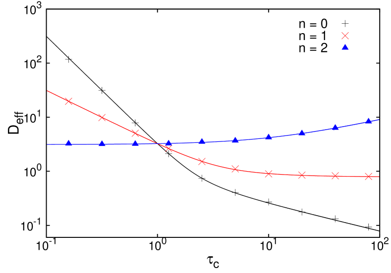
Figure 3: (Color online) The effective diffusion coefficients $D_{\text{eff}}$ are depicted as a function of the correlation time $\tau_{c}$ for several $n$ values within simulations (points) and theory (Eq. (13); lines). Other parameters as in Fig. 2. While decreasing for $n=0$ and approaching a non-zero constant for $n=1$, $D_{\text{eff}}$ diverges $\propto\sqrt{\tau_{c}}$ for $n=2$, see Eq. (26).

Figure 4: Spatial trajectory within an angular OUP dynamics with constant variance $n=1$ for different correlation times $\tau_{c}$ while the parameters hold as in Fig. 7 but with $\Omega=0$, $n=1$ and the time length $t_{l}=1000$. The trajectories changes qualitatively from a random way being unoriented each moment to an agent performing a waltzing-like dance. The effective diffusion coefficient remains unchanged for the shown cases (cf. Fig. 3).

The different crossover behaviors thus reflect the different scaling properties of $D_{\text{eff}}$ for the different regimes of $\Psi_{0}$ in agreement with the result that

$$\mathrm{if}\quad\Psi_{0}\;< \;1\qquad\rightarrow\qquad D_{\text{eff}}\;\approx\frac{v_{0}^{4}\tau_{c}^{n-2}}{2D_{\xi}},$$ (26)

$$\mathrm{if}\quad\Psi_{0}\;> \;1\qquad\rightarrow\qquad D_{\text{eff}}\;\approx\;\frac{v_{0}^{3}}{2}\sqrt{\frac{\tau_{c}^{n-1}}{D_{\xi}}}\,.$$ (27)

Figure 5: Spatial trajectories of an OUP-driven angle without additional torque ($\Omega=0$) at constant $n=2$, $D_{\xi}=0.01$, and $v_{0}=0.5$ for different correlation times $\tau_{c}$ and the time length $t_{l}=1000$. We see a slight growth in the effective displacement for the larger correlation times as also presented in Fig. 3.

This all is in perfect accordance to the numerical results, as depicted in Fig. 3. We notice the strong qualitative changes in the motion of agents which are induced by different $n$. While for $n=0$ and $n=1$, the effective displacement decreases with the correlation time, it even increases with $\tau_{c}$ for $n=2$. That the diffusion coefficient increases unbounded with $\propto\sqrt{\tau_{c}}$ can be seen also in Eq. (20) where, as mentioned in the last paragraph above, the integrand increases monotonously with $\Psi_{0}$, which is the only parameter dependent on $\tau_{c}$ for $n=2$.

On the other hand, regarding the limit $\tau_{c}\rightarrow 0$, $D_{\text{eff}}$ diverges for $n<2$. Only for $n=2$, the diffusion coefficient remains finite and converges to the result of Mikhailov and Meinköhn mikhailov . We notice that the effective noise intensity to which our particles are subjected (i.e., $D_{\xi}/\tau_{c}^{n}$) increases with $n$ for correlation times smaller than one, and decreases with $n$ for correlation times larger than one. For $\tau_{c}=1$ the diffusion coefficient of the three cases merge to the same value. In case of $n=1,2$ for smaller correlation times an effectively larger noise changes the orientation of the particles repeatedly compared to $n=0$. That is why the diffusion coefficient is reduced and is largest for $n=0$. On the other hand, the effective noise intensity acts in the opposite way for $\tau_{c}>1$ leading to a reduced diffusion in case of $n=0$.

Figure 4 depicts for $n=1$ different trajectories for a vanishing torque and $n=1$ within the $\tau_{c}$ region where $D_{\text{eff}}$ changes only marginally (see Fig. 3). Thus, we recognize qualitative changes of the motion, which are just induced by the growth in correlation time, while the variance of the OUP [Eq. (10)] stays constant. One sees that the structure of the trajectory changes from an uncorrelated random sequence to a waltzing like motion where longer straight pieces of the trajectory are interrupted by left- and right-turning pirouettes. We can interpret this behavior as an increment of the trajectories’ persistence as $\tau_{c}$ increases.

Figure 5 depicts trajectories for $n=2$, while $\Omega=0$ still holds. Conforming to the behavior shown in Fig. 3, the displacement slightly increases for the larger correlation time, due to the decreasing variance [see Eq. (10)], which induces a straighter motion. Therefore, the curves also appear smoother for increasing $\tau_{c}$.

III.3 Phenomena of applying finite torque: $\Omega\neq 0$

We next turn to the effects arising from the application of a constant torque. The effective diffusion coefficients are displayed in Fig. 6 for different $n$-values, together with simulation results as a function of increasing color $\tau_{c}$. We observe that the time correlation induces upon varying $\tau_{c}$ a maximal mean square displacement at a finite value of the correlation time for all three cases. A similar graph could be also displayed for the dependence on the noise intensity $D_{\xi}$ (not shown, see also below).

In case that $n=0$, where the integrated noise intensity in the OUP dynamics becomes independent of the color $\tau_{c}$, the maximum is most pronounced. Corresponding trajectories with constant torque are shown in Fig. 7. The curvature of these trajectories reflects the combined influence of the constant torque and of the temporal correlated random torque forces inherent in $\theta(t)$.

For small color $\tau_{c}$ the motion is dominantly circular with small random perturbations. This can be understood in view of Eq. (9), since small correlation times imply strong relaxation so that random changes become essentially white noise with

$$\theta(t)\,\sim\,\sqrt{2D_{\xi}\tau_{c}^{2-n}}\xi(t)\;.$$ (28)

Consequently, in the cases that $n=0$ and $n=1$ the white noise sources tend to vanish. The trajectories follow the motion with the constant torque $\Omega$ along trajectories with a fixed curvature $\propto 1/\Omega$ and therefore $D_{\text{eff}}$ decreases. In contrast to this behavior, Eq. (28) shows that we recover for $n=2$ a white Gaussian angle drive in the limit of small correlation times.

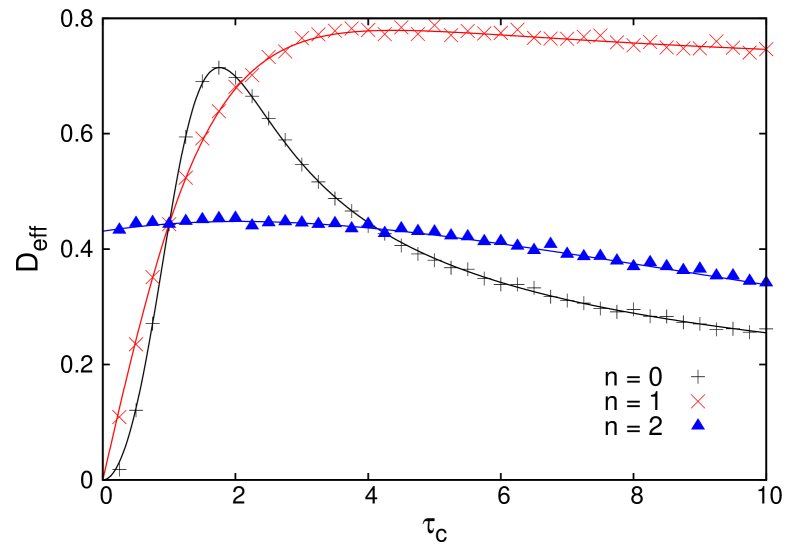
Figure 6: (Color online) Effective diffusion coefficient $D_{\text{eff}}$ versus correlation time $\tau_{c}$ for several $n$-values, a constant torque $\Omega=0.1$, the velocity $v_{0}=0.5$ and $D_{\xi}=0.01$. Simulations (points) agree well with the theory (lines).

For moderate correlation times a modified curled structure emerges. For the stronger correlated systems one observes longer stays at a certain curvature $\theta$ mixed with longer straightening segments where the random torque and the constant torque compensate each other. Thus we retrieve the pirouettes, but now with the preferred curling orientation of the applied constant torques. Thereby the straight segments interrupted by the strongly curling pirouettes give rise to the maximal diffusive behavior and the resonance like structure shown with Fig. 6.

Eventually, for very large correlation times $\tau_{c}$ we find a decrease of the effective diffusion coefficient, much like in the situation without torque [see Fig. (3)]. $D_{\text{eff}}$ converges to zero for $n=0$ and to a non-vanishing constant for $n=1$. The case $n=2$ leads [i.e., due to Eq. (9)] to a dominant torque in the limit of large $\tau_{c}$, so that the effective diffusion coefficient decreases toward $0$.

Figure 7: Spatial trajectories of an OUP driven angle with an additional angular force $\Omega=0.1$, $D_{\xi}=0.01$, $v_{0}=0.5$ and with $n=0$, for different correlation times $\tau_{c}$ and the time length $t_{l}=500$; $n=0$ is used in order to obtain the largest $\tau_{c}$ dependence of the displayed graphs (cf. Fig. 6).

These asymptotic behaviors for small (i.e. $\Psi_{0}\rightarrow 0$) and large correlation times (i.e. $\Psi_{0}\rightarrow\infty$) in Fig. 6 can be discussed analytically in greater detail: According to Eqs. (22) and (23) we arrive at the following limiting behaviors:

$$\mathrm{if}\ \ \Psi_{0}\;\ll \;1\quad\rightarrow\quad D_{\text{eff}}\;\approx\frac{v_{0}^{4}\tau_{c}^{n-2}}{2D_{\xi}}\frac{1}{1+\left(\frac{v_{0}^{4}\Omega}{\tau_{c}^{2-n}D_{\xi}}\right)^{2}},$$ (29)

$$\mathrm{if}\ \ \Psi_{0}\;\gg \;1\quad\rightarrow\quad D_{\text{eff}}\;\approx\;\frac{v_{0}^{3}}{2}\sqrt{\frac{\tau_{c}^{n-1}}{D_{\xi}}}e^{-\frac{v_{0}^{6}\tau_{c}^{n-1}\Omega^{2}}{2D_{\xi}}}.$$ (30)

Thus, we find a vanishing effective diffusion coefficient for correlation times approaching zero if $n\in\{0,1\}$ and one converging to $D_{\text{eff}}^{\text{white}}$, if $n=2$. For large correlation times $\tau_{c}$, on the other hand, we find with $\Psi\gg 1$ that $D_{\text{eff}}^{\text{OUP}}$ converges toward zero if $n=2$ or $n=0$. In distinct contrast, $D_{\text{eff}}$ approaches a constant value for $n=1$.

In comparison to the asymptotic behavior without constant torque [cf. Eqs. (26) and (27)], we notice additional multipliers with dependence on $\Omega$ on the right side of Eqs. (29) and (30). Both multipliers map onto the interval $(0,1)$. Thus, the effective diffusion coefficient always decreases with a constant torque $\Omega\neq 0$. This is depicted in Fig. 8 for $n=0$. As both limits for large and small correlation times fall to zero, a maximal value for $D_{\text{eff}}$ occurs, which not only decreases for growing $\Omega$ but also shifts to larger $\tau_{c}$ .

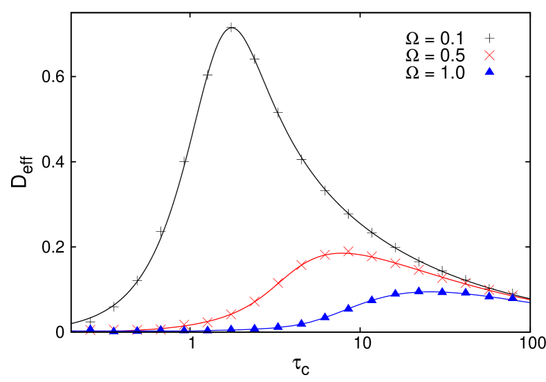
Figure 8: (Color online) Effective diffusion coefficient $D_{\text{eff}}$ versus correlation time $\tau_{c}$ for different torques $\Omega$ at $D_{\xi}=0.01$, $v_{0}=0.5$ and $n=0$, within simulations (points) and in theory [eq. (13); lines].

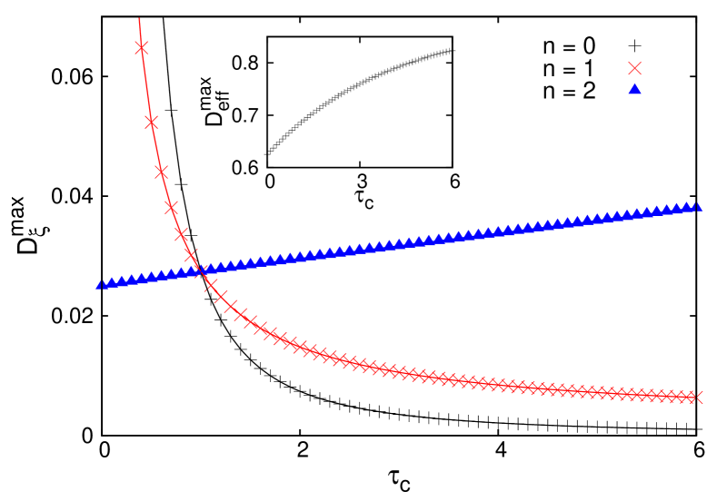
Figure 9: (Color online) Noise intensity $D_{\xi}^{\text{max}}$ which maximizes the effective diffusion constant for a given correlation time for different $n$ at the velocity $v_{0}=0.5$ and the torque $\Omega=0.1$. The inset shows the maximal $D_{\text{eff}}$ for these parameter pairs, which does not depend on $n$.

We now inspect how noise and correlation time influence each other for different $n$. We have seen that the effective diffusion constant exhibits a maximum for a finite non-zero correlation time. Likewise, it has a maximum for a finite non-zero noise intensity, as seen from the results with white noise (see Fig. 1). If we follow the ridge line of the maxima for fixed $\Omega$ in the $(\tau_{c},D_{\xi})$ parameter space, we obtain functional dependencies for different $n$-values, as depicted with Fig. 9. The inset shows the height at the ridge line (i.e., the value for the maximal effective diffusion coefficient as function of the correlation time).

For small $\Omega$, we find that the optimal noise intensity $D_{\xi}^{\text{max}}$, which maximizes the effective diffusion coefficient at a given correlation time, behaves according to $D_{\xi}^{\text{max}}\propto\tau_{c}^{n-2}$. Further analysis shows that for increased $\Omega$ this relation gradually shifts to $D_{\xi}^{\text{max}}\propto\tau_{c}^{n-1-\epsilon}$, with a small finite $\epsilon$. This shift can be justified by the denominator in Eq. (21), in which the second contribution dominates for larger $\Omega$. Figure 9 depicts this dependence for an intermediate value of $\Omega$, since we observe a roughly linear, but still sub-linear, connection for $n=2$, which converges to the value given for a white angle drive as $\tau_{c}\rightarrow 0$. For $n=0$ and $n=1$, we recognize the expected reciprocal connection.

If we follow the ridge line, at a given correlation time each has the same height for different $n$. We can understand this by considering that the parameters $\Psi_{0}$, $\omega_{c}$, and $D_{c}$, which contribute to the effective diffusion coefficient in Eq. (20), are all containing the same factor $D_{\xi}\tau_{c}^{-n}$ as sole $n$ dependence [cf. Eqs. (15) and (19)]. Hence, according to the discussion above, $D_{\text{eff}}$ does not depend on $n$ anymore while regarding $D_{\xi}^{\text{max}}$.

IV Conclusions

With this work the stochastic dynamics of active particles with a constant speed that are additionally driven by an overall fluctuating torque has been studied. The cases of correlated and uncorrelated angle dynamics were considered and analytical results for the mean square displacement were derived. We discussed in this context the dependencies on characteristic parameters of our system, such as the correlation time $\tau_{c}$ and the corresponding noise intensity $D_{\xi}$, to find maxima in the mean square displacement. With respect to the correlation time and to the noise intensity a maximum of the effective diffusion coefficient $D_{eff}$ was identified. We also gave a qualitative explanation of the maximal spreading of the agents by an inspection of the individual trajectories. The random composites of stretched and curved parts in the trajectories can give rise to an increased mean square displacement.

It was also shown that the constant torque decreases the mean square displacement. Therefore, the persistence of motion and presence of a permanent torque are two appropriate instruments to optimize the two-dimensional motion of active agents.

In view of the fact, that the displacement of an agent forms a strong link between theoretical and experimental studies of active particles, we hope that further work within this field benefits from our theoretical reasoning presented here.

Identifying the trajectories of our studied dynamics with the structure of a macromolecule, spin-off applications in the field of polymer physics are conceivable. Especially, the white Gaussian angle drive without a torque has its polymer analog in form of the famous worm-like chain model doi . Moreover, the similarities between the paths in Fig. 7 and Fig. 4 and correlated animal movements are striking for the case of animals, whose angle dynamics is determined by the past states.

Finally, a useful extension of our model would be the adaptation to more realistic biological systems by accounting as well for an additional velocity dynamics $v(t)$. Simple velocity models, wherein one can decouple the $v$- and $\phi$-dynamics, are leading thereby directly to the discussion in peruani , exhibiting a multi-crossover structure of the mean square displacement, which is due to the different time scales within those systems.

- (1) H.U.Bödeker, C. Beta, T. D. Franck, and E. Bodenschatz, EPL 90, 28005 (2010).
- (2) A. Ordemann and G. Balazsi and F. Moss, Physica A 325, 260 (2003)
- (3) J. Gautrais, C. Jost, M. Soria, A. Campo, S. Motsch, R. Fournier, S. Blanco, and G. Theraulaz, J. Math. Biol. 58, 429 (2009).
- (4) A.M. Edwards, et al., Nature 449, 1044 (2007).
- (5) S. Bazazi, J. Buhl, J.J. Hale, M.L. Anstey, G.A. Sword, S.J. Simpson, and I.D. Couzin, Current Biology 18, 735 (2008).
- (6) S. Bazazi et al., Proc. Royal Soc. B: Biological Sciences 278, 356 (2011).
- (7) F. Schweitzer, W. Ebeling, B. Tilch, Phys. Rev. Lett. 80, 5044 (1998).
- (8) A.S. Mikhailov and V. Calenbur, From Cells To Societies: Models of Complex Coherent Action (Springer, Berlin 2001).
- (9) F. Schweitzer, Brownian Agents and Active Particles: Collective Dynamics in the Natural and Social Sciences (Springer, Berlin 2003)
- (10) J. Strefler, W. Ebeling, E. Gudowska-Nowak, and L. Schimansky-Geier, Eur. Phys. J. B 72, 597 (2009).
- (11) P. Romanczuk and L. Schimansky-Geier, to be printed in Phys. Rev. Lett. (2011).
- (12) A. Einstein, Annalen Physik (Leipzig) 322, 549 (1905).
- (13) M. von Smoluchowski, Annalen Physik (Leipzig) 326, 756 (1906).
- (14) P. Langevin, C. R. Acad. Sci. (Paris) 146, 530 (1908); translated an commented on by: D.S. Lemons and A. Gythiel, Am. J. Phys. 65, 1079 (1997).
- (15) Z. Kanokov, J.W.P. Schmelzer, and A.K. Nasirov, CEJP 8, 667 (2010).
- (16) B.M. Friedrich and F. Jülicher, New J. Phys. 10, 123025 (2008).
- (17) B.M. Friedrich and F. Jülicher, Phys. Rev. Lett. 103, 68102 (2009).
- (18) R. Wehner and M.V. Srinivasan, J. Comp. Physiol. 142, 142 (1981).
- (19) M. Müller and R. Wehner J. Comp. Physiol. A 175, 525 (1994).
- (20) P. Romanczuk and I.D. Couzin and L. Schimansky-Geier, Phys. Rev. Lett. 102, 10602 (2009).
- (21) L. Schimansky-Geier, U. Erdmann, and N. Komin, Physica A 351, 51 (2005).
- (22) S. van Teeffelen and H. Löwen, Phys. Rev. E 78, 020101 (2008).
- (23) L. Haeggqwist, L. Schimansky-Geier, I.M. Sokolov, and F. Moss, Eur. Phys. J.– ST 157, 33 (2008).
- (24) S. van Teeffelen, U. Zimmermann, H. Löwen, Soft Matter 5, 4510 (2009).
- (25) G.E. Uhlenbeck and L.S. Ornstein, Phys. Rev. 36, 823 (1930).
- (26) W. Horsthemke and R. Lefever, Noise Induced Transitions, Theory and Applications in Physics, Chemistry and Biology (Springer, Berlin, 1983).
- (27) P. Hänggi, Z. Physik B 31, 407 (1978).
- (28) P. Hänggi, F. Marchesoni, and P. Grogolini, Z. Physik B 56, 333 (1984).
- (29) L. H’walisz, P. Jung, P. Hänggi, P. Talkner, L. Schimansky-Geier, Z. Physik B 77, 471 (1989).
- (30) P. Hänggi and P. Jung, Adv. Chem. Phys. 89, 239 (1995).
- (31) M. Doi and S.F. Edwards, The Theory of Polymer Dynamics (Oxford University Press, 1988).
- (32) I. Sendiña-Nadal, S. Alonso, V. Pérez-Muñuzuri, M. Gómez-Gesteira, V. Pérez-Villar, L. Ramírez-Piscina, J. Casademunt, J. M. Sancho, and F. Sagués, Phys. Rev. Lett. 84, 2734 (2000).
- (33) W. Blum, W. Riegler, L. Rolandi, Particle Detection with Drift Chambers, 2nd ed. (Springer, Berlin, 2008).
- (34) P. Hänggi, Z. Phys. B 36, 271 (1980).
- (35) H.G. Othmer, S.R. Dunbar and W. Alt, J. Math. Biology 26, 263 (1988).
- (36) A.S. Mikhailov and D. Meinköhn, in Stochastic Dynamics, ed. by L. Schimansky-Geier and T. Pöschel, p. 334 (Springer, Berlin 1997).
- (37) S. Chandrasekhar, Rev. Mod. Phys. 15, 1 (1943).
- (38) P. Degond and S. Motsch, J. Stat. Phys. 131, 989 (2008).
- (39) F. Peruani and L.G. Morelli, Phys. Rev. Lett. 99, 10602 (2007).