An $O(N^{3})$ implementation of Hedin’s $GW$ approximation

Abstract

Organic electronics is a rapidly developing technology. Typically, the molecules involved in organic electronics are made up of hundreds of atoms, prohibiting a theoretical description by wavefunction-based ab-initio methods. Density-functional and Green’s function type of methods scale less steeply with the number of atoms. Therefore, they provide a suitable framework for the theory of such large systems.

In this contribution, we describe an implementation, for molecules, of Hedin’s $GW$ approximation. The latter is the lowest order solution of a set of coupled integral equations for electronic Green’s and vertex functions that was found by Lars Hedin half a century ago.

Our implementation of Hedin’s $GW$ approximation has two distinctive features: i) it uses sets of localized functions to describe the spatial dependence of correlation functions, and ii) it uses spectral functions to treat their frequency dependence. Using these features, we were able to achieve a favorable computational complexity of this approximation. In our implementation, the number of operations grows as $N^{3}$ with the number of atoms $N$.

koval.peter@gmail.com1

d.foerster@cpmoh.u-bordeaux1.fr3

sqbsapod@sq.ehu.es1

Centro de Física de Materiales CFM-MPC Centro Mixto CSIC-UPV/EHU and DIPC, E-20018 San Sebastián, Spain

CPMOH/LOMAUniversity of Bordeaux, France

1 Introduction

The promising field of organic electronics deals with large molecules of several tens or even hundreds of atoms [1]. For instance, fullerene C₆₀ is a frequently used subunit in organic electronics and it alone consist of 60 atoms (see figure 1).

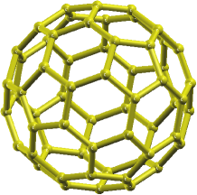
Figure 1: Ball and stick model of fullerene C₆₀ produced with XCrysDen package [2].

Each individual molecule may be used in a device in many different ways and there is an astronomically large number of different promising molecules. As in many cases there is a limited knowledge of the relevant physical parameters, and it might be also interesting to explore the potential of candidate molecules theoretically, before these molecules has been actually synthesised.

The geometry of large organic molecules can be reliably predicted by density-functional theory (DFT)[3]. However, the properties of their excited states such as the energy of the highest occupied (HOMO) and lowest unoccupied molecular orbitals (LUMO), corresponding to adding and subtracting one electron from the system respectively, require a description of electronic correlations better than that provided by current functionals of DFT and its time-dependent counterpart, TDDFT.

Such effects can be efficiently incorporated with the help of Hedin’s method that is based on Green’s function. Hedin’s $GW$ approximation for one-electron Green’s function is computationally cheaper than wavefunction-based methods, although it remains computationally more expensive than DFT and TDDFT within linear response.

The goal of our work is to develop a practical algorithm for Hedin’s $GW$ approximation which is suitable for large organic molecules, allowing to access the excited states of such molecules.

2 Theoretical framework for Hedin’s $GW$ approximation

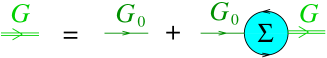
Figure 2: Feynman diagram of Dyson equation (1).

Electronic Green’s function (propagators) are useful in condensed matter physics because many simple observables can be computed in terms of them. At the same time, such Green’s functions remain simpler than many-body wavefunction.

Hedin’s $GW$ is a useful approximation for the so-called self-energy $\Sigma(\bm{r},\bm{r},\omega)$ that enters Dyson’s equation for an interacting electronic propagator $G(\bm{r},\bm{r}^{\prime},\omega)$

$$G^{-1}(\bm{r},\bm{r}^{\prime},\omega)=G_{0}^{-1}(\bm{r},\bm{r}^{\prime},\omega)-\Sigma(\bm{r},\bm{r},\omega).$$ (1)

Here, the inversions must be understood in operator sense $\int G^{-1}(\bm{r},\bm{r}^{\prime\prime},\omega)G(\bm{r}^{\prime\prime},\bm{r}^{\prime},\omega)dr^{\prime\prime}=\delta(\bm{r}-\bm{r}^{\prime})$ and $G_{0}(\bm{r},\bm{r}^{\prime},\omega)$ stands for Green’s function where electron-electron interactions have been switched off. It is obtained from an effective one-particle Hamiltonian

$$(\omega-H(\bm{r}))G_{0}(\bm{r},\bm{r}^{\prime},\omega)=\delta(\bm{r}-\bm{r}^{\prime}).$$ (2)

In this work we use a Kohn-Sham Hamiltonian [3], although Hartree-Fock Hamiltonian also proves to be useful at this point [4]. Hedin’s $GW$ approximation for the self-energy $\Sigma(\bm{r},\bm{r},\omega)$ reads

$$\Sigma(\bm{r},\bm{r}^{\prime},t)=\mathrm{i}G_{0}(\bm{r},\bm{r}^{\prime},t)W_{0}(\bm{r},\bm{r}^{\prime},t).$$ (3)

Figure 3: Feynman diagram of self-energy (3).

It involves the non interacting electronic Green’s function $G_{0}(\bm{r},\bm{r}^{\prime},t)$ and a screened Coulomb interaction $W_{0}(\bm{r},\bm{r}^{\prime},t)$. This approximation is a solution of a truncated version Hedin’s equations [5, 6]. The name of this approximation is taken from the simple form of the electronic self-energy $\Sigma=\mathrm{i}GW$.

The screened Coulomb interaction $W_{0}$ can be easily calculated in frequency domain using the so-called RPA approximation [7]

$$W_{0}(\bm{r},\bm{r}^{\prime},\omega)=\left[\delta(\bm{r}-\bm{r}^{\prime\prime\prime})-v(\bm{r},\bm{r}^{\prime\prime})\chi_{0}(\bm{r}^{\prime\prime},\bm{r}^{\prime\prime\prime},\omega)\right]^{-1}v(\bm{r}^{\prime\prime\prime},\bm{r}^{\prime}),$$ (4)

Figure 4: Feynman diagram of screened Coulomb interaction (4).

where $v(\bm{r},\bm{r}^{\prime})\equiv|\bm{r}-\bm{r}^{\prime}|^{-1}$ is the bare Coulomb interaction. Here and in the following we assume integration over repeated spatial coordinates ($\bm{r}^{\prime\prime}$ and $\bm{r}^{\prime\prime\prime}$ in equation (4)) on the right hand side of an equation if they do not appear on its left hand side. The screened interaction (4) is the sum of the bare Coulomb interaction created by a point charge at $\bm{r}^{\prime}$, plus a correction due to the redistribution of charge induced in response to the total field [7, 6]. The non-interacting response function $\chi_{0}(\bm{r},\bm{r}^{\prime},t)$ is related to the non-interacting Green’s function

$$\mathrm{i}\chi_{0}(\bm{r},\bm{r}^{\prime},t)=2G_{0}(\bm{r},\bm{r}^{\prime},t)G_{0}(\bm{r}^{\prime},\bm{r},-t),$$ (5)

where a factor $2$ arises because of the summation over spin variable.

As we mentioned already, we construct the non-interacting Green’s function using an effective Kohn-Sham Hamiltonian [3]

$$H_{\mathrm{\mathrm{KS}}} =-\frac{1}{2}\nabla^{2}+V_{\mathrm{KS}},$$ (6)

$$V_{\mathrm{KS}} =V_{\mathrm{ext}}+V_{\mathrm{Hartree}}+V_{\mathrm{xc}}\text{, where }V_{\mathrm{xc}}(\bm{r})=\frac{\delta E_{\mathrm{xc}}}{\delta n(\bm{r})}.$$

$E_{\mathrm{xc}}$ is a functional of the electronic density that includes the effects of exchange and correlation in an effective way. Its functional derivative $V_{\mathrm{xc}}(\bm{r})$ is the so-called exchange-correlation potential and it must be subtracted from $\Sigma(\bm{r},\bm{r}^{\prime},t)$ to avoid including the exchange-correlation interaction twice in equation (3). This is accomplished with the substitution

$$\Sigma(\bm{r},\bm{r}^{\prime},t)\rightarrow\Sigma(\bm{r},\bm{r}^{\prime},t)-\delta(\bm{r}-\bm{r}^{\prime})\delta(t)V_{\mathrm{xc}}(\bm{r})$$

in Dyson’s equation (1).

3 A basis set of localized functions

Having the equations (1,3,4,5) at hand we introduce a basis set of localized functions and rewrite the system of equations in the basis. We start with linear combinations of atom orbitals (LCAO) to represent the non-interacting Green’s function $G_{0}(\bm{r},\bm{r}^{\prime},t)$

$$G_{0}(\bm{r},\bm{r}^{\prime},t)=\sum_{ab}G^{0}_{ab}(t)f^{a}(\bm{r})f^{b}(\bm{r}^{\prime}),$$ (7)

where $f^{a}(\bm{r})$ are atom centered orbitals. The frequency (and time) dependence has been factorized in the last equation. The treatment of the frequency (and time) dependence by spectral functions will be explained in section 4. Inserting equation (7) into the equation (5), we obtain

$$\mathrm{i}\chi_{0}(\bm{r},\bm{r}^{\prime},t)=2\sum_{abcd}G^{0}_{ab}(t)G^{0}_{cd}(-t)\,f^{a}(\bm{r})f^{d}(\bm{r})\,f^{b}(\bm{r}^{\prime})f^{c}(\bm{r}^{\prime}).$$ (8)

Products of localized orbitals such as $f^{a}(\bm{r})f^{d}(\bm{r})$ appear in the last equation. Although a product of localized orbitals is also a localized function, such products do not form a suitable basis because they contain many collinear functions. Several methods have been proposed to construct more efficient basis to span the products of localized orbitals [4, 9, 10]. Here we use a basis of dominant products [11] that is constructed individually for each atom pair. The dominant products are identified as certain linear combinations of the original orbital products and they are free of any collinearity within a given atom pair (with respect to a given metric, here we have used the Coulomb metric). Moreover, the original orbital products can be expressed as linear combinations of dominant products

$$f^{a}(\bm{r})f^{b}(\bm{r})=V^{ab}_{\mu}F^{\mu}(\bm{r}).$$ (9)

The three-index coefficient $V^{ab}_{\mu}$ will be referred to as the product vertex. The product vertex is local or sparse by construction and indeed the locality of our construction is its main characteristic.

Considering Dyson’s equation (1), we arrive at its tensor counterpart

$$G_{ab}(\omega)=G^{0}_{ab}(\omega)+G_{aa^{\prime}}(\omega)\Sigma^{a^{\prime}b^{\prime}}(\omega)G^{0}_{b^{\prime}b}(\omega),$$ (10)

where matrix elements of the self-energy $\Sigma^{ab}(\omega)$ must be used

$$\Sigma^{ab}(\omega)=\iint f^{a}(\bm{r})\Sigma(\bm{r},\bm{r}^{\prime},\omega)f^{b}(\bm{r}^{\prime})\,d^{3}rd^{3}r^{\prime}.$$ (11)

Calculating the matrix elements of the self-energy by equation (3) and using (7) for the non interacting Green’s function, we arrive at

$$\Sigma^{ab}(\omega)=\mathrm{i}\sum_{a^{\prime}b^{\prime}}G^{0}_{a^{\prime}b^{\prime}}(t)\int f^{a}(\bm{r})f^{a^{\prime}}(\bm{r})W_{0}(\bm{r},\bm{r}^{\prime},t)f^{b^{\prime}}(\bm{r}^{\prime})f^{b}(\bm{r}^{\prime})\,d^{3}rd^{3}r^{\prime}.$$ (12)

Using the identity (9), we rewrite the latter equation as

$$\Sigma^{ab}(\omega)=\mathrm{i}G^{0}_{a^{\prime}b^{\prime}}(t)V^{aa^{\prime}}_{\mu}W_{0}^{\mu\nu}(t)V^{b^{\prime}b}_{\nu},$$ (13)

where the matrix elements of the screened Coulomb interaction appear

$$W_{0}^{\mu\nu}(t)=\iint F^{\mu}(\bm{r})W_{0}(\bm{r},\bm{r}^{\prime},t)F^{\nu}(\bm{r}^{\prime})\,d^{3}rd^{3}r^{\prime}.$$ (14)

Finally, the equation (4) gives rise to the corresponding tensor expression

$$W_{0}^{\mu\nu}(\omega)=(\delta^{\mu}_{\nu^{\prime}}-v^{\mu\mu^{\prime}}\chi^{0}_{\mu^{\prime}\nu^{\prime}}(\omega))^{-1}v^{\nu^{\prime}\nu}.$$ (15)

The last expression can be elucidated by developing the operator $\left[1-v\chi_{0}\right]^{-1}$ in a geometric series $\left[1-v\chi_{0}\right]^{-1}=1+v\chi_{0}+v\chi_{0}v\chi_{0}+v\chi_{0}v\chi_{0}v\chi_{0}\ldots$ The expressions (8), (10), (13) and (15) are tensor counterparts of Hedin’s equations in coordinate space (5), (1), (3) and (4), correspondingly. In the next section, we will present our method for treating the frequency (and time) dependence of these tensor equations.

4 Spectral function technique

Because of the discontinuities of the electronic Green’s functions, a direct, straightforward and accurate computation of the response function (8) is practically impossible both in the time domain and in the frequency domain. However, one can use an imaginary time technique [12] or spectral function representations to recover a computationally feasible approach. In this work, we use spectral function techniques and rewrite the time ordered operators as follows

$$G^{0}_{ab}(t) =-\mathrm{i}\theta(t)\int_{0}^{\infty}ds\,\rho_{ab}^{+}(s)e^{-\mathrm{i}st}+\mathrm{i}\theta(-t)\int_{-\infty}^{0}ds\,\rho_{ab}^{-}(s)e^{-\mathrm{i}st};$$ (16)

$$\chi^{0}_{\mu\nu}(t) =-\mathrm{i}\theta(t)\int_{0}^{\infty}ds\,a_{\mu\nu}^{+}(s)e^{-\mathrm{i}st}+\mathrm{i}\theta(-t)\int_{-\infty}^{0}ds\,a_{\mu\nu}^{-}(s)e^{-\mathrm{i}st};$$

$$W_{0}^{\mu\nu}(t) =-\mathrm{i}\theta(t)\int_{0}^{\infty}ds\,\gamma_{+}^{\mu\nu}(s)e^{-\mathrm{i}st}+\mathrm{i}\theta(-t)\int_{-\infty}^{0}ds\,\gamma_{-}^{\mu\nu}(s)e^{-\mathrm{i}st};$$

$$\Sigma^{ab}(t) =-\mathrm{i}\theta(t)\int_{0}^{\infty}ds\,\sigma_{+}^{ab}(s)e^{-\mathrm{i}st}+\mathrm{i}\theta(-t)\int_{-\infty}^{0}ds\,\sigma_{-}^{ab}(s)e^{-\mathrm{i}st},$$

where “positive” and “negative” spectral functions define the whole spectral function by means of Heaviside functions $\theta(t)$. For instance, the spectral function of the electronic Green’s function reads

$$\rho_{ab}(s)=\theta(s)\rho^{+}_{ab}(s)+\theta(-s)\rho^{-}_{ab}(s).$$

Transforming the first of equations (16) to the frequency domain, we obtain the familiar expression for the spectral representation of a Green’s function

$$G^{0}_{ab}(\omega)=\int_{-\infty}^{\infty}\frac{\rho_{ab}(s)\,ds}{\omega-s+\mathrm{i}\,\mathrm{sgn}(s)\varepsilon}.$$ (17)

Here $\varepsilon$ is a small line-broadening constant. In practice, the choice of $\varepsilon$ is related to the spectral resolution $\Delta\omega$ of the numerical treatment.

As first application of representations (16), we derive the spectral function of the non interacting response $a_{\mu\nu}(s)$ using equation (5) as a starting point

$$a_{\mu\nu}^{+}(s)=\iint V_{\mu}^{ab}\rho_{bc}^{+}(s_{1})V_{\nu}^{cd}\rho_{da}^{-}(-s_{2})\delta(s_{1}+s_{2}-s)ds_{1}ds_{2}.$$ (18)

Here, the convolution can be computed with fast Fourier methods and the (time-ordered) response function $\chi_{\mu\nu}^{0}(\omega)$ can be obtained with a Cauchy transformation

$$\chi_{\mu\nu}^{0}(\omega)=\chi_{\mu\nu}^{+}(-\omega)+\chi_{\mu\nu}^{+}(\omega),\text{ where }\chi_{\mu\nu}^{+}(\omega)=\int_{0}^{\infty}ds\,\frac{a_{\mu\nu}^{+}(s)}{\omega+\mathrm{i}\varepsilon-s}.$$ (19)

The calculation of the screened interaction $W_{0}^{\mu\nu}(\omega)$ must be done with functions, rather than with spectral functions, because of the inversion in equation (15). The spectral function of the screened interaction $\displaystyle\gamma^{\mu\nu}(\omega)$ can be easily recovered from the screened interaction itself [6]. Since $\mathrm{Im}\frac{1}{\omega+\mathrm{i}\varepsilon-s}$ is a representation of Dirac $\delta$-function when $\varepsilon$ goes to zero, then $\displaystyle\gamma^{\mu\nu}(\omega)=-\frac{1}{\pi}\mathrm{Im}\,W_{0}^{\mu\nu}(\omega)$.

Deriving the spectral function $\sigma(\omega)$ of the self-energy, we arrive at

$$\sigma_{+}^{ab}(s) =\int_{0}^{\infty}\,\int_{0}^{\infty}\delta(s_{1}+s_{2}-s)\,V_{\mu}^{aa^{\prime}}\rho_{a^{\prime}b^{\prime}}^{+}(s_{1})V_{\nu}^{b^{\prime}b}\gamma_{+}^{\mu\nu}(s_{2})ds_{1}ds_{2},$$ (20)

$$\sigma_{-}^{ab}(s) =-\int_{-\infty}^{0}\,\int_{-\infty}^{0}\delta(s_{1}+s_{2}-s)V_{\mu}^{aa^{\prime}}\rho_{a^{\prime}b^{\prime}}^{-}(s_{1})V_{\nu}^{b^{\prime}b}\gamma_{-}^{\mu\nu}(s_{2})ds_{1}ds_{2}.$$

These expressions show that the spectral function of a convolution is given by a convolution of the corresponding spectral functions.

4.1 Discretization of frequency-dependent quantities

The spectral functions in equation (18) are merely a set of poles at (eigen)energies $E$

$$\rho_{ab}^{+}(\omega)=\sum_{E>0}\delta(\omega-E)X_{a}^{E}X_{b}^{E},\ \rho_{ab}^{-}(\omega)=\sum_{E<0}\delta(\omega-E)X_{a}^{E}X_{b}^{E}.$$ (21)

Here the eigenvectors $X_{a}^{E}$ diagonalize the corresponding Kohn-Sham Hamiltonian

$$H^{ab}X_{b}^{E}=ES^{ab}X_{b}^{E},$$

where the Hamiltonian and the overlap matrices of atomic orbitals $f^{a}(\bm{r})$ enter

$$H^{ab}=\int f^{a}(\bm{r})H(\bm{r})f^{b}(\bm{r})d^{3}r,\text{ and }S^{ab}=\int f^{a}(\bm{r})f^{b}(\bm{r})d^{3}r.$$ (22)

In practice, we use the SIESTA package [13] that gives the orbitals $f^{a}(\bm{r})$, eigenvectors $X_{a}^{E}$ and eigenvalues $E$ for a given molecule as the output of a DFT calculation.

The use of fast Fourier techniques for convolution, for instance in equation (18), requires that the spectral functions $\rho_{bc}^{+}(\omega)$, $\rho_{da}^{-}(\omega)$ be known at equidistant grid points $\omega_{j}=j\Delta\omega,j=-N_{\omega}\ldots N_{\omega}$, rather than at a set of energies resulting from a diagonalization procedure. The solution for this problem (discretization of spike-like functions) is known and well tested [14]. We define a grid of points that covers the whole range of eigen energies $E$. Going through the poles $E$, we assign their spectral weight $X_{a}^{E}X_{b}^{E}$ to the neighboring grid points $n$ and $n+1$ such that $\omega_{n}\leq E<\omega_{n+1}$ according to the distance between the pole and the grid points $\displaystyle p_{n,\,ab}=\frac{\omega_{n+1}-E}{\Delta\omega}X_{a}^{E}X_{b}^{E},\ p_{n+1,\,ab}=1-p_{n,\,ab}.$ Such a discretization keeps both the spectral weight and the center of mass of a pole. It also reduces the number of operations that are needed to calculate the non interacting response function $\chi_{\mu\nu}^{0}(\omega)$. This is so because the number of frequencies $N_{\omega}$ can be kept small (typically a few hundred points) even for large molecules while the number of states $N_{\mathrm{orb}}$ grows linearly with the size of the system.

4.2 The second window technique

The discretization of spectral weight helps to control the computational complexity for large molecules. However, we are actually interested in the properties of low lying levels (HOMO and LUMO and several levels below and above). At first sight one might think that one could neglect the contributions of high energy spectral weights in the Cauchy transformation. However, neglecting the high energy spectral weight actually results in a wrong real part of the functions. Fortunately, the high energy spectral weight tolerates a coarser grid [8]. Therefore, we calculate each spectral function twice: once with a higher resolution in a low frequency range, and a second time with a lower resolution but in the whole range. The Cauchy transformation for such a two-window representation must be modified as follows

$$\chi_{\mu\nu}^{0}(\omega+\mathrm{i}\varepsilon_{\text{small}})=\int_{-\lambda}^{\lambda}ds\frac{a_{\mu\nu}(s)}{\omega+\mathrm{i}\varepsilon_{\text{small}}-s}\ +\left(\int_{-\Lambda}^{-\lambda}+\int_{\lambda}^{\Lambda}\right)ds\frac{a_{\mu\nu}(s)}{\omega+\mathrm{i}\varepsilon_{\text{large}}-s}\\ =\chi_{\mu\nu}^{\text{small window}}(\omega+\mathrm{i}\varepsilon_{\text{small}})+\left[\chi_{\mu\nu}^{\text{large window}}(\omega+\mathrm{i}\varepsilon_{\text{large}})\right]_{\text{truncated spectral function}}.$$ (23)

After the calculation of spectral functions in both windows, we truncate the spectral function in the second window in the range $0\ldots\lambda$, do Cauchy transform of both spectral functions and update (by a linear interpolating procedure) the function in the first window with the truncated function from the second window.

We use the second window technique both for the non interacting response function $\chi_{\mu\nu}^{0}(\omega)$ and for the self-energy $\Sigma^{ab}(\omega)$.

5 Non-local compression of the product basis

The basis of dominant products is optimal within a given atom pair, but unfortunately, there is still a lot of collinearity between dominant products belonging to different pairs. This collinearity is an indication that the size of the product basis can be strongly reduced. Even for the molecules of modest size considered in Section 7.1 the basis set of dominant product becomes so large that hampers the storage of the (non-interacting) response function (19) and slows down the inversion in the calculation of the screened interaction (15). In order to improve the situation we perform a non-local (global) contraction of the basis of dominant product. We start by considering a sum-over-states expression for the non-interacting response function in the basis of dominant products

$$\chi_{\mu\nu}^{0}(\omega)=2\sum_{E,F}V_{\mu}^{EF}\frac{n_{F}-n_{E}}{\omega+i\varepsilon-(E-F)}V_{\nu}^{EF}\text{, where }V_{\mu}^{EF}=X_{a}^{E}V_{\mu}^{ab}X_{b}^{F}.$$ (24)

The response $\chi_{\mu\nu}^{0}(\omega)$ is built up from vectors $V_{\mu}^{EF}$ that represent electron-hole pair excitations. One can use these vectors to identify important directions in the space of dominant products. The number of electron–hole pairs $EF$ grows as $N^{2}$ with the molecular size while the dimension of dominant product basis is $O(N)$ by construction (due to the localization of the basis orbitals). Therefore, one has to limit the set of electron-hole pairs $EF$ from the beginning to keep the efficiency of the algorithm, particularly if one uses a diagonalization-based procedure for generating the (globally) optimal basis. Because of the inherent limitations of LCAO to represent high energy features, and the fact that we are mainly interested in the lowest lying excitations, we choose $O(N)$ low-energy electron-hole pairs

$$\{X_{\mu}^{n}\}\equiv\text{subset of }\{V_{\mu}^{EF}\}\text{ limited by }|E-F|<E_{\mathrm{threshold}},n=1\ldots N_{\mathrm{rank}}.$$ (25)

After the initial selection according to the energy criterion $|E-F|<E_{\mathrm{threshold}}$, we define a metric $g^{mn}$

$$g^{mn}=X_{\mu}^{m}v^{\mu\nu}X_{\nu}^{n},\text{ where }v^{\mu\nu}=\iint F^{\mu}(\bm{r})|\bm{r}-\bm{r}^{\prime}|^{-1}F^{\mu}(\bm{r}^{\prime})d^{3}rd^{3}r^{\prime}.$$ (26)

After diagonalizing the metric $g^{mn}\xi_{n}^{\lambda}=\lambda\xi_{m}^{\lambda}$, we can identify important directions (like in the construction of the basis of dominant products [11, 15]) by building linear combinations of the original vectors $X_{\mu}^{m}$ and by choosing only eigenvectors with eigenvalues above a suitable threshold value

$$Z_{\mu}^{\lambda}\equiv X_{\mu}^{m}\xi_{m}^{\lambda}/\sqrt{\lambda}.$$ (27)

These linear combinations can be used to expand the original response function $\chi_{\mu\nu}^{0}(\omega)$ in terms of fewer functions

$$\chi_{\mu\nu}^{0}(\omega)=Z_{\mu}^{m}\chi_{mn}^{0}(\omega)Z_{\nu}^{n}.$$ (28)

In order to express $\chi_{mn}^{0}(\omega)$ in terms of $\chi_{\mu\nu}^{0}(\omega)$ we multiply equation (28) with $Z_{\mu}^{m}v^{\mu\nu}$ from both sides and notice that $Z_{\mu}^{m}v^{\mu\nu}Z_{\nu}^{n}\equiv Z_{\mu}^{m}Z_{n}^{\mu}=\delta_{n}^{m}$. Therefore, the response function can be “compressed” by using basis vectors $Z_{n}^{\nu}\equiv v^{\mu\nu}Z_{\nu}^{n}$

$$\chi_{mn}^{0}(\omega)=Z_{m}^{\mu}\chi_{\mu\nu}^{0}(\omega)Z_{n}^{\nu}.$$ (29)

The particular choice of the Coulomb metric $v^{\mu\nu}$ in equation (26) simplifies the computation of the Coulomb screened interaction (15). We can rewrite the equation (15) in terms of a Taylor series

$$W_{0}^{\mu\nu}=v^{\mu\nu}+v^{\mu\mu^{\prime}}\chi_{\mu^{\prime}\nu^{\prime}}^{0}v^{\nu^{\prime}\nu}+v^{\mu\mu^{\prime}}\chi_{\mu^{\prime}\nu^{\prime}}^{0}v^{\nu^{\prime}\mu^{\prime\prime}}\chi_{\mu^{\prime\prime}\nu^{\prime\prime}}^{0}v^{\nu^{\prime\prime}\nu}+\cdots$$ (30)

Inserting here the response function $\chi_{\mu\nu}^{0}$ according to equation (28) and recalling the identity $Z_{\mu}^{m}Z_{n}^{\mu}=\delta_{n}^{m}$, one arrives at

$$W_{0}^{\mu\nu} =v^{\mu\nu}+Z_{m}^{\mu}\chi_{mr}^{0}\left[\delta_{rn}+\chi_{rn}^{0}+\chi_{rs}^{0}\chi_{sn}^{0}+\cdots\right]Z_{n}^{\nu}=$$ (31)

$$=v^{\mu\nu}+Z_{m}^{\mu}\chi_{mn}^{\mathrm{RPA}}Z_{n}^{\nu},\text{ where }\chi_{mn}^{\mathrm{RPA}}\equiv\left(\delta_{mk}-\chi_{mk}^{0}\right)^{-1}\chi_{kn}^{0}.$$

At this point it should be also be noted that the self-energy $\Sigma_{x}^{ab}(\omega)$ that corresponds to the instantaneous part of the screened interaction $v^{\mu\nu}$ is computed separately [6, 8] without any non local compression.

6 Computational complexity of the algorithm

The number of mathematical operations spent in different parts of the approach presented above can be estimated if the dimensions of the corresponding matrices are known. The numbers that determine the complexity of the algorithm are the number of atomic orbitals $N_{\mathrm{orb}}$, the number of dominant functions $N_{\mathrm{prod}}$ and the number of frequencies $N_{\omega}$. The number of orbitals and the number of dominant products are proportional to the number of atoms $N$ by construction. The number of frequencies affects the run time linearly, but it is independent of the number of atoms. The non-local basis of section 5, can be constructed in $O(N^{3})$ operations because $N_{\mathrm{rank}}$ in equation (25) can be kept proportional to number of orbitals. In practical calculations we have found that converged results are achieved with $N_{\mathrm{rank}}\sim 5N_{\mathrm{orb}}$. For large molecules, the number of important eigenvectors $N_{\mathrm{subrank}}$ after dropping small eigenvalues $\lambda$ in equation (27) is approximately $N_{\mathrm{orb}}$. No part of the algorithm scales worse than $O(N^{3})$ [8]. There are several portions of the code where $O(N^{3})$ operations are needed. However, only two of them have an appreciable impact on the run time: the computation of the response function and the computation of the self-energy. Both of them scale as $O(N_{\mathrm{prod}}^{2}N_{\mathrm{subrank}}N_{\omega})$ and give rise to an overall $O(N^{3})$ scaling of the run time.

7 Applications to organic molecules

The methods described in the previous sections were carefully tested on several molecules. In this paper, we present two examples: calculations of HOMO and LUMO levels of three aromatic hydrocarbons (benzene, naphthalene and anthracene) and a calculation of the HOMO and LUMO levels of fullerene C₆₀.

7.1 Aromatic hydrocarbons

From the interacting Green’s function $G_{ab}(\omega)$ we calculate the density of states (DOS) $\rho(\omega)=-S^{ab}\mathrm{Im}G_{ab}(\omega)/\pi$ and we then determine the positions of the HOMO and LUMO levels from the DOS.

Picture	IP, eV	EA, eV
	8.82 (9.25)	-1.43 (-1.12)
	7.58 (8.14)	-0.15 (-0.19)
	6.87 (7.44)	0.73 (0.530)

Table 1: The ionization potentials (IP) and electron affinities (EA) of benzene, naphthalene and anthracene. Experimental data [16] are given in brackets.

The results of this procedure for aromatic hydrocarbons are collected in table 1. One can see that our (LDA+$G_{0}W_{0}$) approach delivers qualitatively correct predictions for the ionization potentials (IP) and electron affinities (EA) of benzene and naphthalene (donors) and anthracene (acceptor). On the other hand, the LUMO of the underlying DFT calculation is always below the vacuum level. The calculations have been done on top of DFT-SIESTA calculations. We used pseudo potentials of Troullier-Martins type [17] and the Perdew-Zunger exchange-correlation functional [18]. We found that rather extended atomic orbitals must be used to achieve converged results in our $GW$ approach. The energy shift parameter [19], that controls the spatial extension of atomic orbitals has been set to 3 meV for benzene, and to 20 meV for naphthalene and anthracene. The spectral functions have been discretized in two energy windows, with each window containing $N_{\omega}=64$ frequency points.

7.2 Fullerene C₆₀

Source	IP, eV	EA, eV
Our LDA+$G_{0}W_{0}$	7.33	2.97
Experimental [16]	7.58	2.65

Table 2: The IP and EA of fullerene C₆₀ calculated with our method and corresponding experimental data.

The fullerene C₆₀ and its derivatives are very popular ingredients in organic semiconductors and extensive experimental data and theoretical computations are available for the basic fullerene. We found that our LDA+$G_{0}W_{0}$ results are in very good agreement with experimental data (see table 2). The computational parameters of this calculation are the same as in subsection 7.1, while the energy shift parameter is chosen to be 15 meV. The number of frequency points was chosen rather large $N_{\omega}=128$ and the calculation has been done with 8 cores of a Nehalem machine (Intel®E5520 2.27GHz, Cache 8M/DDR3 RAM 24GB). The current version of the code consumed 26 hours of wall clock time.

A comparison of DOS calculated with DFT LDA Hamiltonian and with our LDA+$G_{0}W_{0}$ approach is shown in figure 5. Such a result is a typical when Hedin’s $GW$ approach is applied on top of a LDA calculation. $GW$ HOMO has lower energy than DFT HOMO. Therefore, the change density $n(\bm{r})$ will be more localized in the $GW$ calculation. $GW$ LUMO has higher energy than DFT LUMO. Therefore, the change density $n(\bm{r})$ will be more delocalized in the $GW$ calculation.

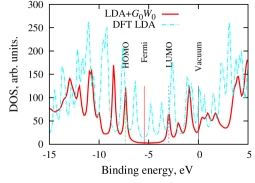
Figure 5: DOS of fullerene C₆₀ computed with our LDA-$G_{0}W_{0}$ approach.

8 Conclusions

We have described our approach to Hedin’s $GW$ approximation for finite systems. This approach allows to compute the interacting Green’s function on a frequency grid. The density of states is our output and it provides HOMO and LUMO levels in reasonable agreement with experiment. The complexity of the approach scales with the third power of the number of atoms, while the needed memory scales with the second power of the number of atoms. These features make our approach suitable for treating the large molecules that are used in organic semiconductors.

References

- [1] See for example the review paper, D. Braga and G. Horowitz, High-Performance Organic Field-Effect Transistors, Adv. Mater. 21 1473 (2009).
- [2] A. Kokalj, Comp. Mater. Sci. 28, 155 (2003).
- [3] P. Hohenberg and W. Kohn, Phys. Rev. 136, B864 (1964); W. Kohn and L. J. Sham, Phys. Rev. 140, A1133 (1965).
- [4] X. Blase, C. Attaccalite, V. Olevano, Phys. Rev. B 83, 115103 (2011); C. Rostgaard, K. W. Jacobsen, and K. S. Thygesen, Phys. Rev. B 81, 085103 (2010).
- [5] L. Hedin, Phys. Rev. 139, A796 (1965). For a review see F. Aryasetiawan and O. Gunnarsson, Rep. Prog. Phys. 61, 237 (1998).
- [6] C. Friedrich and A. Schindlmayr, Many-Body Perturbation Theory: The Approximation, NIC Series, 31, 335 (2006).
- [7] D. Pines, Elementary Excitations in Solids (Wiley, New York, 1964).
- [8] D. Foerster, P. Koval, and D. Sánchez-Portal, arXiv http://arxiv.org/abs/1101.2065, submitted (2011).
- [9] M. E. Casida, in Recent Advances in Density Functional Theory, edited by D. P. Chong (World Scientific, Singapore, 1995, p. 155).
- [10] P. Umari, G. Stenuit and S. Baroni, Phys. Rev. B 79, 201104R (2009); Phys. Rev. B 81, 115104 (2009).
- [11] D. Foerster, J. Chem. Phys. 128, 34108 (2008).
- [12] M. M. Rieger, L. Steinbeck, I. D. White, H. N. Rojas, R. W. Godby, Comp. Phys. Comm. 117, 211 (1999).
- [13] J. M. Soler, E. Artacho, J. D. Gale, A. García, J. Junquera, P. Ordejón and D. Sánchez-Portal, J. Phys.: Condens. Matter 14, 2745 (2002); E. Artacho, E. Anglada, O. Dieguez, J. D. Gale, A. García, J. Junquera, R. M. Martin, P. Ordejón, J. M. Pruneda, D. Sánchez-Portal and J. M. Soler, J. Phys.: Condens. Matter 20, 064208 (2008).
- [14] M. Shishkin and G. Kresse, Phys. Rev. B 74, 035101 (2006); D. Foerster and P. Koval, J. Chem. Phys. 131, 044103 (2009).
- [15] F. Aryasetiawan and O. Gunnarsson, Phys. Rev. B 49, 16214 (1994).
- [16] For hydrocarbons: http://cccbdb.nist.gov/ and J. C. Rienstra-Kiracofe, Ch. J. Barden, Sh. T. Brown, and H. F. Schaefer, J. Phys. Chem. A 105, 524 (2001); for fullerene C60 at http://sesres.com/PhysicalProperties.asp.
- [17] N. Troullier and J. L. Martins, Phys. Rev. B 43, 1993 (1991).
- [18] J. P. Perdew and A. Zunger, Phys. Rev. B 23, 5048 (1981).
- [19] J. Junquera, Ó. Paz, D. Sánchez-Portal, and E. Artacho, Phys. Rev. B 64, 235111 (2001).
- [20] J. D. Talman, J. Chem. Phys. 80, 1984 (2000); J. Comput. Phys. 29, 35 (1978); Comput. Phys. Commun. 30, 93 (1983); Comput. Phys. Commun. 180, 332 (2009).