Accurate Modeling of the Cubic and Antiferrodistortive Phases of SrTiO₃ with Screened Hybrid Density Functional Theory

Abstract

We have calculated the properties of SrTiO₃ (STO) using a wide array of density functionals ranging from standard semi-local functionals to modern range-separated hybrids, combined with several basis sets of varying size/quality. We show how these combination’s predictive ability varies significantly, both for STO’s cubic and antiferrodistortive (AFD) phases, with the greatest variation in functional/basis set efficacy seen in modeling the AFD phase. The screened hybrid functionals we utilized predict the structural properties of both phases in very good agreement with experiment, especially if used with large (but still computationally tractable) basis sets. The most accurate results presented in this study, namely those from HSE06/modified-def2-TZVP, stand as the most accurate modeling of STO to date when compared to the literature; these results agree well with experimental structural and electronic properties as well as providing insight into the band structure alteration during the phase transition.

I Introduction

Strontium titanate (SrTiO₃; STO) is a complex oxide perovskite of great technological interest for its superconductivity,Ueno et al. (2008) blue-light emission,Kan et al. (2005) photovoltaic effect,Zhou et al. (2009) and so on. Under normal conditions, bulk SrTiO₃ crystallizes in a cubic perovskite structure; it subsequently undergoes a second order phase transition at $T_{c}$=105 K to a tetragonal structure with slightly rotated oxygens around the z-axis, known as the antiferrodistortive (AFD) phase (see Fig. 1). Many of the interesting properties of STO, either in bulk or in superlattices formed with other metal oxides, are believed to be caused by the cubic to AFD phase transition. Examples of this attribution are STO’s superlattice’s high T_c superconductivity Reyren et al. (2007); Caviglia et al. (2008); Kozuka et al. (2009) and its colossal magnetoresistivity. Gao et al. (2009) First-principles calculations (see Ref. Pentcheva and Pickett, 2010 and references therein) have indicated that the strain-induced competition between octahedral rotation modes and the lattice distortion in metal oxide superlattices are behind these interesting properties. Thus, there is a considerable need Borisevich et al. (2010); Chang et al. (2010) for precise theoretical calculations of the structural and electronic properties of complex oxides, as well as accurate estimation of the phase transition order parameters, to understand and eventually exploit these phenomena.

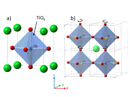
Figure 1: (Color online) SrTiO₃ unit cells for the a) cubic phase and b) antiferrodistortive phase; b) shows the TiO₆ octahedra’s rotation around the [001] axis. Sr atom are in green, Ti are in blue and O are in red. The O₁ (equatorial) and O₂ (axial) labels denote the non-rotating and rotating oxygens, respectively.

The phase transition of STO is governed by two order parameters. The primary order parameter is the rotation angle of the TiO₆ octahedra ($\theta$). The experimentally measured Unoki and Sakudo (1967) octahedral rotation of AFD STO is 1.4° at 77 K and increases as the temperature drops toward the maximum measured value of 2.1° at 4.2 K. The octahedron’s rotation is believed to be almost complete Jauch and Palmer (1999) at around 50 K, where $\theta$=2.01$\pm$0.07° was reported. The secondary order parameter is the tetragonality of the unit cell ($c/a$), which increases from 1.00056 Cao et al. (2000) to 1.0009 Heidemann and Wettengel (1973) as the temperature decreases from 65 K to 10 K. The AFD phase can also appear in thin films of STO He et al. (2004, 2005, 2003) at much higher T_c than the bulk, depending on the substrate used, the thickness of deposited STO film, the strain and the lattice mismatch. For example, 10 nm of STO deposited on LaAlO₃ (LAO) undergoes a transition to the AFD phase at $T_{c}\cong$ 332 K.

As the simplest metal oxide perovskite, STO has been extensively studied in the last decades with different ab initio schemes.Zhukovskii et al. (2009); Eglitis and Vanderbilt (2008); Heifets et al. (2006a); Wahl et al. (2008) However, it is still a challenging material for theory; only a few of the previously published works have been able to accurately describe the structural and electronic properties of the both phases of STO. The balance of this section will consist of a brief review of the theoretical work performed to date.

Sai and Vanderbilt Sai and Vanderbilt (2000) carried out one of the first LDA calculations on STO using a plane-wave basis and ultra-soft pseudopotentials. LDA predicted an exaggerated tetragonal AFD phase of STO, with octahedral rotation angles of 6°, significantly overestimating the 2.1° rotation measured experimentally. Unoki and Sakudo (1967) Using LDA with other basis sets Uchida et al. (2003) shows similar issues, predicting rotations up 8.4°.

Wahl et al. Wahl et al. (2008) used a plane-wave basis while simulating STO with LDAVosko et al. (1980), PBE Perdew et al. (1996, 1997) and PBEsol.Staroverov et al. (2003, 2004) (See Section II for further descriptions of these density functionals). LDA underestimated experimental lattice constants, while PBE overestimated them; both methods had band-gaps that were seriously underestimated compared to experiment. This underestimation is well known for these functionals; see e.g. Ref. Mori-Sánchez et al., 2008 and references therein. PBEsol was found to reproduce accurately the experimental structure, but considerably underestimated the band gaps. For the AFD phase, the octahedral angle $\theta$ was found to be very sensitive to the functional used; all three overestimate the AFD deformation, with LDA worse than PBE and PBEsol splitting the difference. Rondinelli et al. Rondinelli and Spaldin (2010) applied the LSDA+$U$ correction to cubic STO and found that while it corrects the band gap, the calculated octahedral rotation angle remains overestimated at 5.7°. To date, none of the post-DFT corrections which benefit band-gaps have successfully corrected the octahedral rotation overestimation, and many authors attribute this to the argument proposed by Sai and Vanderbilt Sai and Vanderbilt (2000) stating that this can be caused by the exchange and correlation terms in DFT not capturing quantum point fluctuations.

Piskunov et al. Piskunov et al. (2004) conducted one of the most complete and comprehensive ab initio studies of STO, using Gaussian basis sets specifically optimized for modeling STO crystals. This study of STO showed problems when modeling with pure DFT or pure HF, namely underestimated and overestimated band gaps, respectively; this is a well known problem.Janesko et al. (2009) Hybrid functionals, specifically B3PWBecke (1993) and B3LYP,Lee et al. (1988) gave more reasonable results, with direct band gaps overestimated by 5% for B3PW and 3.5% for B3LYP compared to experiment and indirect band gaps overestimated by 12% for B3PW and 10% for B3LYP. (We will demonstrate that an important part of this overestimation can be attributed to the basis set employed; see section III.) The hybrid functionals also gave the best agreement with experiment for the lattice constant and the bulk modulus, and generally did better than semilocal functionals in all categories. This success of hybrid functionals motivated more detailed calculations Zhukovskii et al. (2009); Eglitis and Vanderbilt (2008); Heifets et al. (2006a) of the properties of the cubic and AFD phases of STO, again using the optimized basis set of Piskunov et al. Piskunov et al. (2004) and the B3PW functional.

Next, Wahl et al. Wahl et al. (2008) applied the Heyd-Scuseria-Ernzerhof Heyd et al. (2003, 2006) screened Coulomb hybrid density functional (HSE) in a plane-wave basis set. HSE performed exceptionally well, doing much better than any of semilocal functionals, as it gave a very accurate estimate of both the structural and electronic properties of the cubic phase. HSE also showed excellent agreement with the experimental octahedral angle and tetragonality of the unit cell which constitute, to our knowledge, the most accurately computed STO properties available in the literature for both phases, prior to the current study.

As noted above, hybrid functionals have proved their effectiveness in studying metal oxides, but they are computationally much more demanding than semilocal functionals. While it would be ideal to do high accuracy ab initio on metal oxide superlattices using complete basis sets and large supercells, this is prohibitively expensive at the current level of computer power. Screened hybrid functionals with only short range exact exchange are computationally less demanding; they allow the use of large supercells, especially when used with localized basis sets such as Gaussian functions. We hope to use the most effective methods/basis sets from this study on more complicated metal oxide systems, and thus we have concentrated on methods and basis sets that would be practical for those systems as well as the systems currently under consideration.

This paper focuses on two tightly linked problems. We are interested in the degree of completeness (or size) of the localized basis set necessary to correctly simulate both phases of STO, and in the efficacy of recently developed functionals (including screened hybrids) in predicting the properties of STO. To discuss these issues, the paper proceeds as follows: In Section II, we briefly describe the technical details before turning in Section III to the basis set optimization/modification technique we used to make standard basis sets PBC-compatible. In Section IV, we report the results of semilocal and range separated hybrid functionals applied to the cubic and the AFD phases of STO. We show also how the quality of basis set affected the accurate prediction of the octahedral rotation angle in the AFD phase of STO. Finally, we discuss the results of our best functional/basis set combination for STO, comparing them with previously published theoretical and experimental data, with special emphasis on the effect of varying the range separation parameter in the screened functionals.

II Computational Details

All calculations were performed using a development version of the Gaussian suite of programs,Frisch et al. with the periodic boundary condition (PBC)Kudin and Scuseria (2000, 1998a, 1998b) code used throughout. A wide array of functionals were applied, including: the Local Spin Density Approximation Vosko et al. (1980) (LSDA), the generalized gradient approximation (GGA) corrected functional of Perdew, Burke and Ernzerhof Perdew et al. (1996, 1997) (PBE), the reparametrization of PBE for solids, PBEsol, Staroverov et al. (2003, 2004) the revised meta-GGA of Tao, Perdew, Staroverov and ScuseriaTao et al. (2003); Perdew et al. (2009) (revTPSS), and finally a modern and highly parametrized meta-GGA functional, M06L. Zhao and Truhlar (2006, 2008) Two screened hybrid functionals were also tested, namely the short-range exact exchange functional of Heyd, Scuseria, and Ernzerhof Krukau et al. (2006); Heyd et al. (2003) (HSE, with the 2006 errata, also referred to as HSE06) and the exact exchange in middle-range functional of Henderson, Izmaylov, Scuseria, and Savin (HISS).Henderson et al. (2007, 2008) Because regular hybrids with unscreened exact exchange like B3LYP and B3PW have higher computational cost compared to screened hybrids we decided to exclude them from this test.

Gaussian basis sets of different quality have been tested for their ability to simulate the properties of STO; the details of these tests and the modification of the basis set was detailed enough to merit its own section, section III.

A few numerical considerations should be mentioned here. During the initial (or exploratory) calculations for the AFD phase, we found some dependence of octahedral rotation angle ($\theta$) on initial atomic positions. After further investigation, this can be attributed to the geometric optimization convergence criteria. Since $\theta$ is so small, very stringent convergence criteria is required. Another modified (versus the default) setting was that a pruned integration grid for DFT of (99, 590) was employed, which corresponds to the Gaussian option “ultrafine”. Note that this grid is big enough for this system to avoid any of the instabilities with M06L reported in the literature with small grids.Johnson et al. (2009); Wheeler and Houk (2010) To ensure this, we tested M06L with a larger grid, without noticing any modification in the calculated properties. Thus while “ultrafine” is sometimes insufficient for M06L, it is not for this system. Other numerical settings in gaussian were left at the default values, e.g. integral cut-offs, k-point meshes, SCF convergence criterion, and the like.

Finally, the geometry of each phase is worth discussing briefly. The starting configuration for the cubic phase (see Figure 1(a)) consisted of the perovskite primitive cell containing 5 atoms at the experimental lattice constant Abramov et al. (1995) ($a_{0}$= 3.890 Å). For the AFD phase, we couldn’t simply use the 5 atom tetragonal unit cell with rotated oxygens and the lattice parameters set to $a=b\neq c$. A 20 atoms supercell/simulation cell was necessary, as the phase transition requires a rotation of every pair of neighboring TiO₆ octahedra in opposite directions (figure 1(b)). Thus, the volume of the AFD supercell is about four times the volume of the cubic phase with tetragonal lattice constants $a^{*}=b^{*}=\sqrt{2}a$ and $c^{*}=2c$, with $a$ and $c$ being the lattice parameters of the 5 atoms tetragonal unit cell in the AFD phase. The starting AFD structure of STO was taken from the experimental structure of Jauch et al. Jauch and Palmer (1999) obtained at 50 K and downloaded as CIF file from the ICSD,ICS with $a^{*}=b^{*}=5.507$ Å and $c^{*}=7.796$ Å. The starting rotation angle for TiO₆ octahedra was 2.1° while the $c/a-1=10\times 10^{-4}$. Please note the geometries were only starting points; as mentioned above all geometries were optimized with the method/basis set under consideration. In order to avoid introducing any errors coming from size effects or k-space integration, the calculated properties of the AFD supercell are always compared with a 20 atoms supercell constructed from four cubic primitive cells (without octahedral rotation or tetragonality) fully relaxed using the same k -point mesh. It should be noted that the supercell in the cubic phase is a local minimum and is higher in energy than the supercell in the AFD phase for all reported calculations. The final (reported) $\theta$ values were determined from Ti-O₂-Ti angle measurements, and any octahedral tilts can be estimated by measuring the Ti-O₁-Ti angles (O_n’s subscript was defined in Figure 1). Finally, all geometric visualization was done using GaussView. Dennington et al.

III Basis set efficiency for SrTiO₃

The challenge in selecting a basis set is always balancing accuracy with computational cost. In molecular calculations, the computational cost of a gaussian basis set is determined by the number of functions used, while in PBC calculations the spatial extent or diffuseness of the basis set also plays a major role. The more diffuse a basis set is, the larger the chunk of matter that must be included in the calculations to avoid numerical issues.

Coupled with the argument that the long density tail is more necessary for molecular work than work in extended systems, it becomes obvious that basis sets developed for non-periodic calculations can require modification for PBC use. This section describes the basis set optimization/modification procedure we employed to find the appropriate Gaussian basis sets to simulate periodic STO while keeping within reasonable computational expense. We based our evaluations of a basis set’s accuracy on cubic STO results using the Heyd-Scuseria-Ernzerhof Heyd et al. (2003, 2006) screened Coulomb hybrid density functional (HSE06). Krukau et al. (2006)

The obvious starting point was the basis sets used in previous calculations/studies of bulk STO, including:

• Gaussian-type basis sets published by Piskunov et al. Piskunov et al. (2000) in 2000, optimized using the Hartree-Fock (HF) and density functional theory (DFT) with Hay-Wadt pseudopotentials Hay and Wadt (1984a, b, c) for Sr and Ti, denoted here as P1.
  

• The subsequently improved version of P1 published by Piskunov et al. Piskunov et al. (2004) in 2004, which expands of P1 by adding polarization d-functions to oxygen and making the Ti s and p functions more diffuse, denoted here as P2.

Table 1: The electronic and structural properties of cubic SrTiO₃  computed with HSE06 Krukau et al. (2006) and different basis sets. Please see the text for basis set naming conventions.

Basis set	P1	P2	SZVP	TZVP	Experiment
Direct gap (eV)	3.87	3.80	3.59	3.59	3.75
Indirect gap (eV)	3.53	3.46	3.18	3.20	3.25
a0(Å)	3.900	3.908	3.887	3.902	3.890, 3.900
B(GPa)	198	194	204	193	179,
					179$\pm{4.6}$

Tests on P1 and P2 were done with HSE06, because it has been found to give the best results versus experiment for both structural and electronic propertiesWahl et al. (2008) in older calculations. Both P1 and P2 reproduce the experimental equilibrium lattice constants Abramov et al. (1995) (see Table 1) almost perfectly. Cubic STO modeled with P1  has a slightly higher bulk modulus compared to P2, although the difference between the two basis sets in fairly minimal for structural properties. A more important effect is observed for the electronic properties: P1 and P2 overestimate the direct band gap of STO by 0.12 and 0.05 eV respectively, and seriously overestimate the indirect band gap by 0.28 and 0.21 eV.

It is easy to see that the P2 basis set employed with HSE06 lead to results that are closer to experiment than P1, a fact noted by PiskunovPiskunov et al. (2004) for a number of functionals. The more important point is that increasing the size/quality of the basis set made a noticeable change in the results; the immediate question is whether another increase in basis set size would bring about similar improvement. In other words, using polarization d-orbitals for O and diffuse functions for Ti improved the HSE06 results, and imply that further improvement could potentially be achieved if more basis set improvements are implements, e.g. including titanium core electrons and/or adding more diffuse functions for oxygen.

We decided to optimize some of the Def2- Weigend and Ahlrichs (2005) series of Gaussian basis sets for use in bulk STO calculations. The original Def2- basis sets for the atoms of interest in this project included small-exponent diffuse functions ($\alpha_{min}$ less than 0.10) that are spatially quite extended; as stated above, this long tail is necessary to improve the DFT results for molecules but not necessary for crystals. Heyd et al. (2005); Strain et al. (1996) Basis sets with large spatial ranges dramatically slow down the calculation of Coulomb contributions to the total energy of crystals. Thus, to be useful in PBC calculations, Def2- basis sets must be modified by removing some of the most diffuse functions.

The series of Def2- basis sets are available up to quadruple zeta valence quality for a large set of elements.Weigend and Ahlrichs (2005); Weigend (2006) In the original optimizations, the oxygen, strontium and titanium basis sets were optimized (using HF and DFT) versus the properties of SrO, TiO and TiO₂ molecules. Strontium has the inner shell electrons replaced with small core pseudopotentials, Kaupp et al. (1991) while the other two atoms utilize all electron basis sets; this differs from P1 and P2 which uses pseudopotentials on titanium as well. In general, Def2- basis sets are larger and more expensive than P1 and P2 basis sets, but are expected to give a better representation of both phases of STO due to greater “completeness.”

To make a Def2- basis set applicable to PBC, the first step is selecting a maximum allowable diffuseness, or equivalently the smallest acceptable Gaussian orbital exponent, $\alpha_{min}$. The larger the value of $\alpha_{min}$, the faster the calculations become, but if $\alpha_{min}$ is set too high, significant degradation of physical property prediction results. After the threshold is defined, one pass is made through the basis set to reset all $\alpha<\alpha_{min}$ to $\alpha_{min}$, and then a second pass is made through the basis set to remove any redundancies. Note that after modifying or deleting an element of a contracted basis set, we rely on the code’s internal renormalization code, i.e. no attempt is made to reoptimize contraction coefficients.

We first began with the largest Def2- basis sets, Def2-QZVP and Def2-QZVPP, but these were found to be computationally intractable for bulk STO even for $\alpha_{min}$ as big as 0.2, and previous experience have shown that $\alpha_{min}$ larger than 0.2 causes physically unacceptable results. We then moved to the smaller basis sets, Def2-TZVP and Def2-SZVP. We first set $\alpha_{min}$= 0.12, but found this made the calculations very slow. Our tests showed that $\alpha_{min}$= 0.15 constitutes a more computationally efficient choice without important loss in accuracy.

Henceforth, the Def2-TZVP and Def2-SZVP, with $\alpha_{min}$ modified and redundant s functions removed, will be denoted TZVP and SZVP, respectively.

Table 1 summarizes the calculated electronic and structural properties of cubic STO using our basis set modifications as well as the aforementioned P1 and P2. The optimized basis sets SZVP and TZVP give an overall excellent agreement with experiment: Abramov et al. (1995) direct band gaps are now underestimated by 0.16 eV while indirect band gaps are now underestimated by $\sim$0.05 eV. These two new basis sets are larger than the previously utilized P1 and P2, are more accurate for indirect gaps, as well for other measured properties, and due to their greater size are expected to be closer to the upper limit of HSE06 accuracy for this system. Note also that the electronic properties of STO remain almost unchanged by moving from a SZVP to TZVP basis set. The deviation from the experimental lattice constant do not exceed 0.07 and 0.3% for SZVP and TZVP respectively but is more substantial for the bulk modulus reaching 14% for SZVP and 8% for TZVP. Finally, the same series of basis set optimizations were also performed using HISS and M06L functionals, which lead to the same conclusions regarding the basis set efficiency; these are not presented here for space reasons.

Before moving on to the results section, a brief mention of the expense of the various basis sets should be included. In term of relative CPU time, one SCF cycle takes about 12 units for TZVP compared to 6 units for SZVP and 1 unit for P2. All of these basis sets still have potential uses; SZVP or P2, for example, might be very useful for a rapid investigation of the electronic properties of some complex STO systems. But, in term of completeness, TZVP is the most complete and the closest to the planewave basis set limit, followed by SZVP, then P2.

IV Results: Basis set and functional evaluation

In this section we present the calculated properties of SrTiO₃, always discussing the results of each functional using the TZVP basis set first, followed with a discussion of the sensitivity of the functionals to smaller basis sets, namely SZVP and P2.

IV.1 Structural properties of cubic SrTiO₃

Table 2: Computed lattice parameter $a_{0}$(Å) and bulk modulus B(GPa) for Cubic STO using different combinations of functionals and basis sets compared to experiment.

	HSE06	HISS	M06L	revTPSS	LSDA	PBE	PBEsol	Experiment
a0(Å)								3.890, 3.900
TZVP	3.902	3.883	3.925	3.921	3.862	3.941	3.897
SZVP	3.887	3.869	3.909	3.903	3.845	3.924	3.881
P2	3.908	3.891	3.930	3.920	3.870	3.946	3.903
B(GPa)								179,
TZVP	193	206	187	180	201	169	184	179$\pm{4.6}$
SZVP	204	218	198	193	214	180	196
P2	194	205	191	184	203	173	187

The calculated equilibrium lattice constants and the bulk moduli of cubic STO using different functionals and basis sets are reported in Table LABEL:tab:ela-cub. Unless specified, the deviation of theory from experiment will be always referred to the data of Abramov et al, Abramov et al. (1995) i.e. treated as the target value. Focusing first on the TZVP results, we observe that the screened hybrids HSE06 and HISS give lattice parameters in excellent agreement with experiment.

The calculated bulk modulus using HSE06 is fairly close to the experimentally reported values, although overestimated by 8%. (The same magnitude of overestimation have been also reported in the HSE planewave calculations of Wahl et al. Wahl et al. (2008).) However, a larger bulk modulus overestimation of 15% is observed for HISS, which constitutes the largest deviation from experiment among all the studied functionals.

M06L and revTPSS predict slightly higher equilibrium lattice constants than screened hybrids do, but their bulk moduli are closer to experiment, with revTPSS being especially close. LSDA underestimates the lattice constant by 0.03 Å, while PBE predicts lattice constants 0.05 Å larger than experiment. PBEsol is in excellent agreement with the experimental lattice constant. Thus PBEsol corrects the LSDA underestimation and the PBE overcorrection to LSDA for lattice constants; in addition, the PBEsol bulk modulus deviate by less than 3% from experiment, while LSDA and PBE are off by 11% and 12%, respectively. This is an example of PBEsol meeting its purpose, as it improves the PBE lattice constant and bulk modulus for the cubic phase, approaching very closely the experimental data.

Turning now to the functional sensitivity to basis set size, we observe from the HSE06 results that SZVP basis set predict bond lengths that are very slightly shorter than the TZVP and a bulk modulus that is  6% higher. As such, SZVP predicts SrTiO₃ to be 14% harder than experiment. P2 behave in the opposite direction, predicting slightly longer bonds when compared to TZVP, while the bulk moduli are only 1GPa higher. From table LABEL:tab:ela-cub, this sensitivity of HSE06 to smaller basis set can be generalized to M06L, revTPSS and the semilocal functionals LSDA, PBE and PBEsol.

Finally, it should be noted that PBEsol results offer the best agreement with experimental structural properties Abramov et al. (1995) of SrTiO₃ among all the studied functionals with the TZVP basis set, followed by the screened hybrid HSE06 and the meta-GGA revTPSS.

IV.2 Electronic properties of cubic SrTiO₃

Table 3: Direct and indirect band gaps computed for Cubic SrTiO₃ using different basis sets and functionals compared to experiment.

	HSE06	HISS	M06L	revTPSS	LSDA	PBE	PBEsol	Experiment
Direct gap(eV)								3.75 van Benthem et al. (2001)
TZVP	3.59	4.39	2.51	2.24	2.08	2.11	2.10
SZVP	3.59	4.45	2.53	2.28	2.12	2.14	2.14
P2	3.80	4.56	2.63	2.52	2.34	2.33	2.34
Indirect gap(eV)								3.25 van Benthem et al. (2001)
TZVP	3.20	3.98	2.09	1.87	1.75	1.74	1.75
SZVP	3.18	4.03	2.10	1.89	1.76	1.75	1.76
P2	3.46	4.22	2.24	2.17	2.04	1.99	2.02

The computed electronic properties of SrTiO₃ are summarized in table LABEL:tab:elec_cub. As expected, HSE06 gives an excellent estimate of the electronic properties when used with the large TZVP basis sets. Deviations from the experimental values are 0.15 eV for the direct gap and 0.05 for the indirect gap. A cursory glance over the rest of table LABEL:tab:elec_cub indicates that no other functional was comparable to HSE06’s efficacy for band gaps, i.e. everything else we tried had much larger errors.

The midle range screened hybrid HISS tend to overestimate the direct and indirect band gaps by 0.35 and 0.73 eV, respectively. M06L and revTPSS tend to underestimate both band gaps, by an average of $\sim$1.2 and $\sim$1.4 eV respectively. The semilocal functionals LSDA, PBEsol, PBE underestimate the experimental band gaps by an average of  45% or 1.5 eV. This was expected, and is in agreement with the behavior observed earlier in the literature for this system. Wahl et al. (2008) It can be easily seen from these results that HSE06 is the best functional choice for investigating this system.

Turning to basis set sensitivity, it can be seen from the HSE06 numbers that band gaps are nearly unaffected by using the smaller SZVP basis sets, but when used with the still smaller P2 basis set, direct and indirect band gaps increase by $\sim$0.25 eV versus TZVP. The predicted direct band gap becomes closer to experiment when using P2 and HSE06, probably due to a cancellation of errors effect, while the indirect band gap is noticeably worse. This same sensitivity holds for almost every other functional, with SZVP and TZVP giving about the same band gaps and P2 opening the band gaps up by a few tenths of an eV. M06L appears to be slightly less sensitive; no obvious reason for this exists.

IV.3 Stability of the AFD phase of STO

This section examines the stability of the AFD phase of STO as calculated by the various functionals and basis sets previously tested for the cubic phase. The functional/basis set combinations tested face the challenge of predicting the AFD octahedral rotation angle, $\theta$, as well as the tetragonality parameter $c/a$, which as shown in section I is not trivial. The AFD phase order parameters are evaluated from the relaxed 20-atoms AFD supercells as described in section II. The performance of each functional with TZVP, and then an analysis of the functional’s sensitivity to the smaller basis sets is presented in turn.

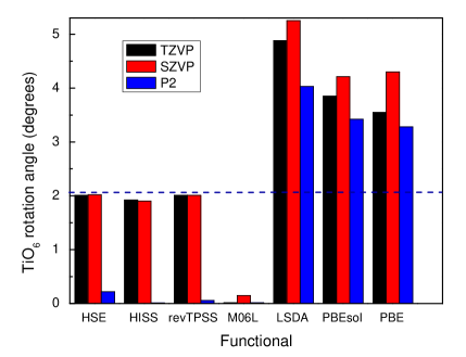
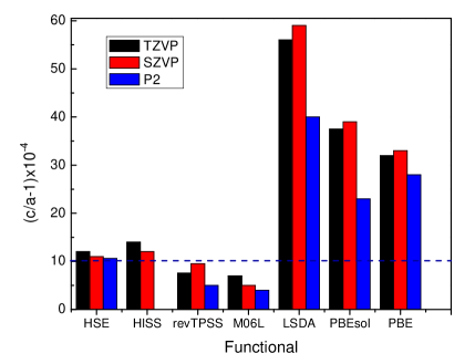
Figure 2: (Color online) Performance of different functional/basis set combinations in predicting the order parameters of the AFD phase transition in STO. Dashed lines depict the experimental octahedral angle measured at 4.2 K from Ref. Unoki and Sakudo, 1967 (left) and the tetragonality parameter obtained at 50 K from Ref. Jauch and Palmer, 1999 (right).

Figure 2 shows that the screened hybrid functional HSE06 is excellent for the structural properties of AFD, as it was for the cubic phase. Both the rotation angle $\theta$ and the $c/a$ ratio are in very good agreement with experiment. These properties are not significantly affected when SZVP is used, but HSE06/P2 predicts a very very small angle for the AFD phase, while retaining a good $c/a$. This is one area where TZVP noticeably outperforms P2  with HSE06.

HISS and revTPSS behave as HSE06 for both TZVP and SZVP, giving a good estimate of both order parameters. However, they demonstrate a higher sensitivity to the smaller P2 basis set and required the use of a very stringent convergence criterium to finally relax the structure back to a pseudocubic phase with $\theta\approx$0. On the other hand, M06L predicts the AFD phase to be unstable, and relaxes to a non-rotated structure regardless of the basis set used.

Table 4: Structural and electronic properties of the antiferrodistorsive phase of SrTiO₃ compared to previously simulated data and experiments. $a^{*}$ and $c^{*}$ are the lattice parameters of the AFD supercell and $c/a=c^{*}/{\sqrt{2}a^{*}}$. $\Delta E=E_{Cubic}-E_{AFD}$ represent the gain in total energy after the cubic to AFD phase transition, while $\Delta E_{g}$ denote the corresponding increase in the band gap.

	LSDA	PBE	PBEsol	HSE06	HISS	revTPSS	M06L	Experiment
$a^{*}$(Å)
Present	5.449	5.568	5.500	5.515	5.448	5.543	5.551	5.507
Ref. Wahl et al., 2008	5.440	5.562	5.495	5.515
$c^{*}$(Å)
Present	7.727	7.900	7.812	7.809	7.772	7.846	7.862	7.796
Ref Wahl et al., 2008	7.755	7.897	7.818	7.808
$(c/a-1)\times 10^{-4}$
Present	27	32	44	12	14	7.6	7	10
Ref. Wahl et al., 2008	80	40	60	10
Others	40
$\theta$(°)
Present	4.14	3.54	3.81	2.01	1.92	2.01	0	2.01$\pm$0.07
Ref. Wahl et al., 2008	6.05	4.74	5.31	2.63				2.1
Others	8.40, 6
	4
$\Delta E\times 10^{-5}$ (eV)
Present	1796	854	44	35	578	258	122
Ref. Wahl et al., 2008	1900	700	1100	200
Indirect band gap (eV)
Present	1.820	1.787	1.808	3.227	3.995	1.890	2.060	3.246 Yamada and Kanemitsu (2010)
Ref. Wahl et al., 2008	1.970	1.790	1.930	3.110				3.160 Hasegawa et al. (2000)
$\Delta E_{g}$ (meV)
Present	75	49	58	27	15	15	30	50
Ref. Wahl et al., 2008	160	10	110	40

The semilocal functionals LSDA, PBEsol and PBE all overestimate the tetragonality of the AFD phase by predicting $\theta$ and $c/a$ almost twice the size of the experimental results. The highest overestimation was observed for LSDA, followed by PBEsol then PBE. Note that our result here is in excellent qualitative agreement with the behavior found in the planewave calculations of Wahl et al; Wahl et al. (2008) quantitatively, however, the LSDA, PBEsol and PBE octahedral angles with TZVP are 25-30% lower than the planewave results Wahl et al. (2008); Sai and Vanderbilt (2000); Uchida et al. (2003) (for a detailed numerical comparison see table 4, and ref. Wahl et al., 2008 has additional comparison with experiment). Similar behavior has been recently published Hong et al. (2010) for LSDA calculation with finite-range numerical atomic orbitals using a double-$\zeta$ polarized basis set. This indicates that localized basis sets tend to reduce the AFD octahedral rotation compared to plane-waves but do not succeed to suppress the DFT overestimation.

When used with the SZVP basis sets, the LSDA, PBE and PBEsol rotation angles are larger than the TZVP ones. Furthermore, when LSDA, PBEsol and PBE are used with the P2 basis set, we observe a small and coherent reduction in the octahedral rotation angle of the AFD structure compared to TZVP results. This demonstrates that semilocal functionals have different degrees of sensitivity to the quality of the localized basis sets used, but the error caused by functional choice is always the more important source of error. Thus the functionals examined here will lead to exaggerated AFD $\theta$ values for all basis sets considered.

V Discussion: Physical properties of STO

Before talking about specific issues, there are a few general conclusions we can reach from examining the results in section IV

1. HSE06/P2 did a good job in describing accurately the structural properties for the cubic phase as well as providing a descent estimation of the band gap. However, the failure of HSE06/P2 to correctly model the structure of the AFD phase indicates that it must be abandoned as a useful combination for this and related systems.

2. HSE06/SZVP has the drawback of predicting a stiffer SrTiO₃ in the cubic phase, although it predicts electronic properties as well as TVZP. It also predicts a stiffer AFD structure, but the octahedral angle and $c/a$ parameters are very good.

3. HSE06/TZVP gave the best agreement with experiment for the cubic phase and for the AFD phase. It is definitely the most reliable combination of functional and basis set among all studied variations. Thus HSE06/TZVP can be used with confidence on more complicated structures, as well as to understand the change in the electronic structure during the cubic to AFD transition for this system. More concisely, we believe that this combination is an accurate enough functional in a good enough basis set to explain phenomena in metal oxides.

Figure 3: Band structure of cubic SrTiO₃  calculated with HSE06/TZVP. The dashed line depict the Fermi level lying at the valence band maximum ($R$ special point.)

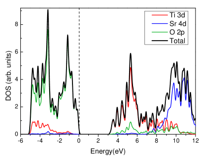
Figure 4: (Color online) Total electronic density of states (DOS) of cubic SrTiO₃ calculated with HSE06/TZVP. Projected density of states (PDOS) of the main contributing orbitals are also shown.

V.1 Band structure alteration by the AFD phase transition

The band structure of the cubic unit cell of STO computed with HSE06/TZVP is shown in figure 3, with the high symmetry points $\Gamma=(0,0,0)$, $X=(0,\frac{1}{2},0)$, $M=(\frac{1}{2},\frac{1}{2},0)$ and $R=(\frac{1}{2},\frac{1}{2},\frac{1}{2})$ labeled, in the first Brillouin zone of the simple cubic system. The dashed line depict the Fermi level lying at the valence band maximum at the $R$ point.

Our band structure agrees qualitatively with previous band structures from LSDA/PW calculations, which can be seen (for example) in Fig. 5 of Ref. Uchida et al., 2003, as well as the B3PW/P2 band structure in Ref. Piskunov et al., 2004 Fig. 2(a), with the exception of a few details. Our direct band gap ($\Gamma\rightarrow\Gamma$) of 3.59 eV and indirect gap ($R\rightarrow\Gamma$) of 3.2 eV are in better agreement with experiment van Benthem et al. (2001) compared to the underestimation observed in the LSDA/PW gaps and the overestimation found with B3PW/P2. Thus for a DFT approach, this diagram is the best band structure to date. (An even more accurate band structure was computed using the experimental lattice constant of SrTiO₃ by mean of post-LSDA quasiparticle self-consistent GW (QSGW) correction to the band structure by Hamann and Vanderbilt.Hamann and Vanderbilt (2009))

Figure 4 shows the total density of states (DOS) as well as the projected density of states (PDOS) on every atomic orbital. The PDOS of oxygen represents the sum of the contributions of all three oxygen atoms in the cubic unit cell. In the energy window shown here, the DOS is dominated by oxygen 2$p$, titanium 3$d$ and strontium 4$d$ states. (All the remaining orbitals have a negligible contribution, so their PDOS are not shown.) The valence band (VB) from 0 to $-$6 eV is dominated by oxygen 2$p$ states, with a small contribution from titanium 3$d$ states in the range $-$3 to $-$6 eV. The conduction band (CB) is clearly dominated by titanium 3$d$ in the energy range 3.2$-$7 eV, with a smaller contribution coming from the 3 oxygen 2$p$ states as well. The admixture in the VB and CB between the titanium 3$d$ and oxygen 2$p$ orbitals demonstrates that the Ti$-$O bonds have a partially covalent character with a small degree of hybridization. (This behavior has been noted in previously published data. Uchida et al. (2003)) Between 7$-$9 eV, the spectrum is the sum of contributions from oxygen 2$p$, titanium 3$d$ and strontium 4$d$ orbitals. The higher energy region in the CB (9$-$12 eV) is dominated by strontium 4$d$ orbitals with small contributions from titanium 3$d$ and with oxygen 2$p$ vanishing at around 10.5 eV.

Figure 5 compares the total electronic densities of states for the cubic and AFD supercells. As a general trend, the cubic to AFD phase transition does not lead to a significant modification in the total DOS; both the valence and the conduction bands experience a slight shift to higher energies (horizontal arrows) together with some small modifications, indicated by vertical black arrows in Figure 5. However, the VB shift does not affect the peak at the VB maximum, while a very small shift to higher energies is observed for the CB minimum, indicating that the band gap increase by $\approx$27 meV after the transition. This same behavior holds for all the functionals/basis sets combinations tested, and is in line with some experimental observations Hasegawa et al. (2000) reporting very small changes in their measured band gaps due to the cubic-to-tetragonal structural transition. Further confirmation of this physical effect can be seen in recent photoluminescence measurements, Yamada and Kanemitsu (2010) which reported that the band gap increased by 50 meV when temperature decreased from 85 K to 8 K, which is a temperature range over which the AFD rotation would go from incomplete to nearly total.

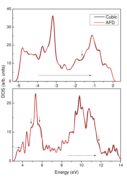
Figure 5: (Color online) Modification in the total DOS of STO upon the cubic to AFD phase transition. Horizontal arrows indicate the direction of the energy shift, while vertical arrows point to the most important changes.

A more detailed comparison between the PDOS for each atomic orbital can give a better understanding of the origin of these modifications. It is important to mention that in the AFD supercell, there is one nonrotating O₁ atom and two rotating O₂ oxygens for every Sr and Ti atom. Concentrating on the oxygen 2$p$ orbitals, we observe that the non-rotating O₁ atoms are nearly unchanged in the PDOS compared to the cubic phase, with the exception of a tiny shift to higher energy (see the inset in Figure 6), which can be attributed to the elongation of the cell along the z-axis. However, the O₂ demonstrate a much more significant shift to higher energies, along with changes in the height and width of some peaks. This is mainly caused by the octahedral rotation involving O₂ atoms. The titanium 3$d$ and strontium 4$d$ spectra experience the same aforementioned shift to higher energies in the VB and the CB due to the elongation of the lattice, with a few noticeable changes in the titanium 3$d$ spectrum at $-$2.9 as well as between 5 and 6.5 eV. Most of the modifications observed in the total DOS, with the exception of few originate from the changes in the O₂ 2$p$ and Ti 3$d$ spectra with the O₂ being far more important.

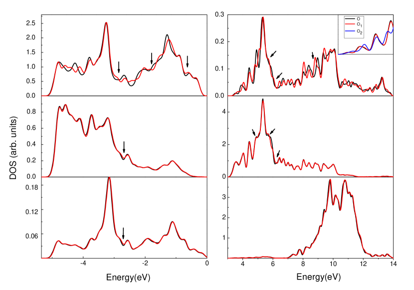
Figure 6: (Color online) Modification of the partial densities of states (PDOS) for O 2p, Ti 3d and Sr 4d Left: Valence band Right: Conduction band

V.2 The effect of the HSE screening parameter, $\omega$

Relying on the assumption that plane-waves are much closer to the infinite basis set limit than the Gaussian basis sets we used, it is useful to compare our HSE06/TZVP results with the HSE plane-wave results. To our knowledge, only Wahl et al. Wahl et al. (2008) have published data using plane-waves and a Heyd-Scuseria-Ernzerhof Heyd et al. (2003, 2006); Krukau et al. (2006) style screened Coulomb hybrid density functional for this system. However, a direct comparison with our present data is not possible because Wahl et al. used a different screening parameter in their calculations.

Briefly, the HSE functional partitions the coulomb potential into short-range (SR) and long-range (LR) components:

$$E^{HSE}_{xc}=\frac{1}{4}E^{HF,SR}_{x}(\omega)+\frac{3}{4}E^{PBE,SR}_{x}(\omega)+E^{PBE,LR}_{x}(\omega)+E^{PBE}_{c}$$ (1)

The screening parameter $\omega$ defines the separation range, as it controls the distance at which the long-range nonlocal interaction becomes negligible, i.e. it “turns off” exact exchange after a specified distance. Wahl et al. used $\omega_{1}$=0.159 $a.u.^{-1}$, effectively using an HSE-style functional, but not either of the functionals HSE03 or HSE06. Krukau et al.Krukau et al. (2006) applied HSE while varying 0.11$\leq\omega\leq$ 0.20 to a number of bulk metals and semiconductors. They concluded that a small increase of $\omega$ substantially lowers the calculated band gaps and the smaller value omega takes in this range, the closer the calculated band gaps and lattice constants are to the experiment. Based on the above, Krukau et al., Krukau et al. (2006) recommended $\omega_{2}$=0.11 $a.u.^{-1}$ for both the HF and PBE part of the exchange. This is the value we used in all our calculations, and this value is part of the formal definition of HSE06. However, in order to make a comparison between our HSE($\omega_{2}$)/TZVP and the HSE($\omega_{1}$)/PW data of Wahl et al., we must perform a HSE/TZVP calculation with $\omega_{1}$ and isolate the screening parameter effect on the calculated properties of SrTiO₃.

Table 5: Variation of the cubic STO lattice parameter(a₀ in Å ), bulk modulus (B in GPa), and direct ($E_{g}^{d}$) and indirect ($E_{g}^{i}$) band gaps (in eV) by decreasing the HSE screening parameter from $\omega_{1}$=0.159 $a.u.^{-1}$ to $\omega_{2}$=0.11 $a.u.^{-1}$. Results are from our Gaussian basis set (TZVP) and the plane-wave (PW) calculations in Ref. Wahl et al., 2008.

	Gaussian		PW		Experiment
	$\omega_{1}\longrightarrow\omega_{2}$		$\omega_{1}\longrightarrow\omega_{2}$
a0	3.903	3.902	3.904	3.903	3.890, 3.900
B	192	193	192	193	179, 179$\pm{4.6}$
$E_{g}^{d}$	3.37	3.59	3.47	3.67	3.75
$E_{g}^{i}$	2.96	3.20	3.07	3.27	3.25

Table LABEL:tab:omega shows that the HSE($\omega_{1}$)/TZVP lattice constant and bulk modulus changes very slightly by decreasing the screening parameter from $\omega_{1}$ to $\omega_{2}$: the change is 0.001 Å  and 1 GPa respectively. A much more significant effect is, however, observed for the band gaps: decreasing the screening parameter by 50% ( $\omega_{1}\rightarrow\omega_{2}$), lead to an increase in the band gaps, effectively a rigid shift of 0.22 and 0.24 eV for the direct and indirect band gaps respectively. If examined from the other direction, decreasing the screening parameter from $\omega_{1}$ to $\omega_{2}$ (with HSE/TZVP) tends to bring the band gaps closer to the experiment (see table LABEL:tab:omega), which suggests that $\omega_{2}$ provides better agreement with experiment than $\omega_{1}$ does. The same structural changes and band gap shifts were also found for the small basis sets SZVP and P2, which are not presented here and which demonstrate that this effect is completely independent from the basis set used. Finally, the HSE($\omega_{2}$)/TZVP band gaps are very close to the HSE($\omega_{2}$)/PW values we estimated, suggesting that our TZVP basis set is very close in quality to the previously used plane waves, and thus is closer to the basis set limit.

This section is contains one of the most important results of this paper, and as such should be clearly restated. If we use the same version of HSE used in plane wave studies, we can show that our TZVP is a high quality basis set as it matches the excellent basis set plane wave results. If we use the proper $\omega$ in HSE with our basis set, we arrive at the best results/smallest errors versus experiment ever reported for SrTiO₃.

Finally, it should be noted that this is not an ad hoc parameterization of $\omega$ to give the best results for this study. We were able to obtain results that closely match experiment by using a demonstrably high quality basis set and a parameter in the density functional determined by a large test bed of structures and properties.Krukau et al. (2006)

V.3 Screened hybrids compared to regular hybrids.

Table 6: Our most converged direct ($E_{g}^{d}$) and indirect ($E_{g}^{i}$) band gaps (in eV) for cubic STO alongside previously published hybrid functional results done with the P2 basis set. Regular hybrids data are corrected according to the basis set sensitivity effect deduced in section IV.2.

	functional/basis	$E_{g}^{d}$		$E_{g}^{i}$
		Ori.	Corr.${}^{\text{estimated}}$	Ori.	Corr.${}^{\text{estimated}}$
Exp. van Benthem et al. (2001)		3.75		3.25
Present	HSE06/TZVP	3.59		3.20
Ref. Piskunov et al.,2004	B3PW/P2	3.96	3.74	3.63	3.35
	B3LYP/P2	3.89	3.67	3.57	3.30
Ref. Heifets et al.,2006b	B3PW/P2	4.02	3.80	3.70	3.42
Ref. Zhukovskii et al.,2009	B3PW/P2	—	—	3.63	3.35
Ref. Bilc et al.,2008	B1-WC/P2	3.91		3.57

Table LABEL:tab:all_litt summarizes the calculated band gaps of HSE06/TZVP and compares them with previously published gaps computed with the regular hybrids B3PW and B3LYP, done with the P2 basis set. There are noticeable differences between the results of HSE06 and the regular hybrids, with HSE06/TZVP giving band gaps very close to experiment while regular hybrids used with P2  overestimate the gap, especially the indirect band gap. The band gap overestimation is of same magnitude we observed in section IV.2 for HSE06/P2 as well as all the other functionals tested on STO with P2. This suggests that P2 is also behind the band gap overestimation in the regular hybrids data reported in the literature.Piskunov et al. (2004); Heifets et al. (2006b); Zhukovskii et al. (2009) By comparing the P2  and TZVP band gaps from table LABEL:tab:elec_cub, we can deduce that the P2  basis set has an effect (versus a large basis set) of increasing the direct and indirect band gaps by average values of 0.22 and 0.28 eV respectively. By applying this P2$\rightarrow$TZVP basis set correction to the regular hybrid B3PW/P2 and B3LYP/P2  band gaps (see the corrected values in table LABEL:tab:all_litt), band gaps are brought closer to the experimental values, and thus closer to the HSE06/TZVP results as well. Consequently, differences in the computed electronic properties of HSE06 and B3PW and B3LYP are considerably attenuated and suggest that the screened hybrid HSE06 is comparable in accuracy with regular hybrids for STO, while being much more computationally efficient.

The final issue to discuss is the comparison of the structural and elastic properties of STO computed with HSE06 versus regular hybrids. Perovskite crystals in the cubic structure have only three independent elastic constants, namely C₁₁, C₁₂ and C₄₄, as well as a bulk modulus:

$$B=\frac{1}{3}(C_{11}+2C_{12})$$ (2)

We calculated the elastic constants of STO using HSE06/TVZP, following the methodology described in Ref. Wu et al., 2005. Ideally we would like to compare our cubic elastic constants calculated at 0 K with low temperature data, but as experimentally the cubic structure turns to a tetragonal structure below a transition temperature, making any comparison of this kind impossible. Experimentally, Bell and Rupprecht Bell and Rupprecht (1963) found that the elastic constants of STO measured between 303 and 112 K obey the following empirical relations:

$$C_{11}=334.1[1-2.62\times 10^{-4}(T-T_{a})-\frac{0.0992}{(T-T_{a})}]$$ (3a)

$$C_{12}=104.9[1-1.23\times 10^{-4}(T-T_{a})+\frac{0.1064}{(T-T_{a})}]$$ (3b)

$$C_{44}=126.7[1-1.30\times 10^{-4}(T-T_{a})-\frac{0.1242}{(T-T_{a})}]$$ (3c)

where the elastic constants are in GPa, T is the temperature and $T_{a}$=108 K is the critical temperature. C₁₁ and C₄₄ reach their maximum values at 133 K where STO is still cubic, then they start to decrease as $-1/(T-T_{a})$ in the region around the transition temperature, in contrast, C₁₂ continue to increase as $1/(T-T_{a})$ in the same temperature range.

Since we don’t know at which temperature the change from cubic to tetragonal phase begins to take place, it is better to limit our comparison with data measured at 133 K and above. Table LABEL:tab:ela summarizes our results and compares them with experiment as well as previously published results with B3PW/P2  and B3LYP/P2. HSE06/TZVP provides excellent lattice constants but predicts the bulk modulus to be 8% higher than experiment. The elastic constants from HSE06/TZVP overestimate the experimental data at room temperature by 10% and the 133 K data by 6%; this was expected given the overestimation of the bulk modulus. The B3PW hybrid also gave very good lattice constant and bulk modulus, but the calculated elastic constants are lower than the room and the low temperature experimental values. B3LYP predicted a lattice constant higher by 1%, a good bulk modulus, and offers the best agreement with the low temperatures elastic constants. In summary, none of the screened or regular hybrids considered was able to give simultaneously excellent bulk moduli and elastic constants, still HSE06/TZVP offer the best compromise between efficiency, accuracy and speed.

Table 7: Calculated elastic constants with HSE06/TZVP for cubic STO compared to experiment and previously published results with the regular hybrid functional B3PW and the P2 basis set from Ref. Piskunov et al., 2004. a₀ is in Å, B, C₁₁, C₁₂ and C₄₄ are in GPa

	$a_{0}$	B	C11	C12	C44
HSE06/TZVP	3.902	193	351.4	113	137.3
B3PW/P2	3.900	177	316	92.7	120.1
B3LYP/P2	3.940	177	328.3	105.7	124.6
Exp.	3.890 Abramov et al. (1995)	179 Abramov et al. (1995)	317.2	102.5	123.5
	3.900 Hellwege and Hellwege (1969)	179$\pm{4.6}$ Fischer et al. (1993)	330	105	126
	3.910	184			128

VI Conclusion

We used the ab-initio code gaussian to simulate the properties of SrTiO₃ (STO) using a large spectrum of functionals, from LSDA, GGAs (PBE and PBEsol) and meta-GGAs (M06L and revTPSS) to modern range-separated hybrid functionals (HSE06 and HISS); assessing their ability in predicting the properties of the cubic and the AFD phases of STO.

We found that pure DFT functionals tend to overestimate the octahedral rotation angles of the AFD phase, in agreement with previously reported results in the literature using plane-wave basis sets of comparable quality. Wahl et al. (2008) Also, basis sets of low quality tend to inhibit the tetragonality of the AFD phase and sometimes even suppress it, regardless of the functional used. We therefore constructed a localized basis set of sufficient completeness (or size) to correctly simulate the TiO₆ octahedral rotation and the cubic phases of STO. We also evaluated the band gap errors arising from the use P2 basis set and from the magnitude of the HSE screening parameter $\omega$. By applying our basis set and $\omega$ corrections to the previously published work with regular and screened hybrid functionals on STO, we showed that the discrepancies between published simulated data can be explained and that hybrid functionals used with sufficiently big Gaussian-type basis sets can give results comparable with plane-wave calculations and in excellent agreement with experiment.

The screened hybrid functional HSE06 predicts the electronic and structural properties of the cubic and AFD phase in very good agreement with experiment, especially if used with high quality basis set TZVP. HSE06/TZVP is the most reliable combination of functional and Gaussian basis set for STO which is computationally tractable with the current computer power. It is accurate enough to enable us to understand the changes in the band structure during the cubic to AFD phase transition. The success of HSE06/TZVP encourages its use on more complicated cases like the bond breaking and over binding and defect formation, where the basis set completeness is expected to play a major role.