VISCOUS COSMOLOGIES WITH VARIABLE $G$ AND $\Lambda$ IN $R^{2}$ GRAVITY

Abstract

We study evolution of a flat Friedmann-Robertson Walker universe filled with a bulk viscous cosmological fluid in a higher derivative theory of gravity in the presence of time varying gravitational and cosmological constant. Cosmological models admitting both power-law and exponential expansions are explored here in the presence of imperfect fluid described by full Israel and Stewart theory. We note some new and interesting cosmological solutions relevant for model building including present accelerating phase. In the case of power law, it is found that gravitational constant increases as the time evolves for a positive cosmological constant whereas it decreases for a negative cosmological constant. The evolution of temperature of a viscous universe is also determined.
PACS No(S): 98.80. Cq

1 Introduction

Recent astronomical observations of type Ia supernovae with redshift parameter $Z\leq 1$ [1], Wilkinson Microwave Anisotropy Probe (WMAP) [2] etc. provided evidence that we may live in a low mass density universe ($\Omega\sim 0.3$) [3]. The predictions of the observations lead to a convincing belief in modern cosmology that a part of the universe is filled up with dark energy ($\Omega\sim 0.7$), which may be addressed by a suitable cosmological constant. One of the recent predictions that the present universe accelerating is remarkable which is not properly understood yet. The present accelerating phase of the universe may be accommodated in cosmological models, obtained from theories : either by a modification of the Einstein’s theory of gravity (GR) or by including a time varying cosmological constant. A number of literature appeared which addressed the present accelerating phase making use of exotic kind of fields in the matter sector of the Einstein’s field equation. The study of late universe however, remains open to address the present issues in other theories. One of the early attempts to modify GR is based on adding curvature squared terms to the Einstein-Hilbert action which is known as generalized theory of gravity was used to obtain early inflation. The theory is found to have a number of good features important for understanding early universe. Starobinsky [4] shown that $R^{2}$ term in the Einstein Hilbert action admits inflation long before the advent of inflation is actually realized. However, the efficacy of the theory is known only after the seminal work on inflation by Guth [5], who employed temperature dependent phase transition mechanism to obtain inflation. The inflationary scenario of the early universe is attractive and which may solve some of the outstanding problems in cosmology [6]. It is known that higher order gravity with suitable counter terms viz., $C^{\mu\nu\rho\delta}C_{\mu\nu\rho\delta}$, $R^{2}$, and cosmological constant ($\Lambda$) added to the Einstein-Hilbert action, one gets a perturbation theory which is well behaved, formally renormalizable and asymptotically free [7, 8].

Cosmological models considering perfect fluid as a source of matter in the framework of higher derivative gravity have been studied in the literature [9] in order to obtain viable cosmological scenario of the early universe. In the absence of particle creation, particle number is conserved in the perfect fluid ( i.e., $n^{\alpha}_{;\alpha}=0$, where $n$ is particle number density ). It may be pointed out here that perfect fluid in equilibrium generates neither entropy ($S^{\alpha}_{;\alpha}=0$) nor frictional heat flow as their dynamics is reversible.

However, in the early universe a number of processes might have occurred leading to a deviation from perfect fluid assumption e.g. viscosity which is to be taken into account. It is known that real fluids behave irreversibly and therefore it is important to consider dissipative processes both in cosmology and in astrophysics. Some of the dissipative processes in the early universe responsible for viscosity may be due to the decoupling of neutrinos from the radiation era, the decoupling of matter from radiation during the recombination era, creation of superstrings in the quantum era, particle collisions involving gravitons, cosmological quantum particle creation processes and formation of galaxies [10]. It has been predicted from observations that a non negligible dissipative bulk stress on cosmological scales at the late universe phase might be important. The possible source of such viscosity may be due to (i) gaseous matter in the framework of relativistic gravity which may give rise to internal self-interaction leading to a negative cosmic bulk pressure [11], (ii) deviation of the non relativistic particle in the substratum from dust. For a non-relativistic substratum cosmic anti-friction may generate a negative fluid bulk pressure which has been noted [12] in the framework of Einstein gravity.

Since the pioneering work of Dirac [13], who proposed a theory with a time varying gravitational coupling constant $G(t)$, a number of literature [14] appeared with variable $G(t)$ and $\Lambda(t)$ in higher derivative theory of gravity in order to obtain cosmological models accommodating the present cosmic acceleration. Recent applications of the apparent magnitude-redshift test, based on type Ia supernovae [2, 15], strongly favours a theory with a positive $\Lambda$ term. A number of ansatze have been proposed for a dynamical decaying $\Lambda$ with time [16]. Berman and collaborators [17] pointed out that cosmological constant may vary as $\Lambda\sim t^{-2}$, which seems to play a major role in cosmology. To obtain a time varying cosmological constant, one can assume different phenomenological relations proportional to the Hubble parameter, one such example [17] considered in recent times is of the form $\Lambda\propto H^{2}$ where $H$ is Hubble parameter. Cosmological models with imperfect fluid have been explored in the presence of a dynamical cosmological constant and gravitational constant in Einstein gravity [18]. It is , therefore, important to look into viable cosmological models with variable $G(t)$ and $\Lambda(t)$ in higher derivative theory of gravity in the presence of imperfect fluid.

To describe a relativistic theory of viscosity, Eckart [19] made the first attempt. However, the theories of dissipation in Eckart formulation suffers from serious shortcoming, viz., causality and stability [20] regardless of the choice of equation of state. The problem arises due to first order nature of the theory, since it considers only first order deviation from equilibrium. It has been shown that the problems of the relativistic imperfect fluid may be resolved by including higher order deviation terms in the transport equation [21]. Israel and Stewart [22], and Pavon [23] developed a fully relativistic formulation of the theory taking into account second order deviation terms in the theory, which is termed as ”transient” or ”extended” irreversible thermodynamics (in short, EIT). The crucial difference between the standard Eckart and the extended Israel-Stewart transport equations is that the latter is a differential evolution equations, while the former is an algebraic relation. Extended irreversible thermodynamics takes its name from the fact that the set needed to describe non-equilibrium states is extended to include the dissipative variables ($\tau$, $\zeta$). In irreversible thermodynamics, the entropy is no longer conserved, but grows, according to the second law of thermodynamics (i.e., $S^{\alpha}_{;\alpha}\geq 0)$. Bulk viscosity arises typically in mixtures either of different species or of the species but with different energies. The solutions of the full causal theory are well behaved for all the times. Therefore, the best currently available theory for analyzing dissipative processes in the universe is the full Israel-Stewart theory (FIS). Using the transport equation obtained from EIT, in addition to dynamical equation obtained from either Einstein gravity [18, 25] or modified gravity [24] cosmological solutions are generally obtained. The motivation of this paper is to explore cosmological solutions in the modified theory of gravity in the presence of variable $G(t)$ and $\Lambda(t)$ with imperfect fluid described by FIS theory. It is interesting to study the behaviour of $G(t)$ and $\Lambda(t)$ in the presence of viscosity.
The characteristic temperature of the universe may be determined in the presence of viscosity in the FIS theory. However, it may be pointed out here that in a number of literature [25] the evolution of temperature of the universe in the presence of viscosity from Gibbs equation is considered in the Einstein gravity. We also consider the above procedure in the framework of higher order gravity to determined the behaviour of temperature.
The plan of this paper is as follows: in sec. 2, we give the gravitational action and set up the relevant field equations in the higher derivative theory of gravity. In sec. 3, cosmological solutions are presented. In sec. 4, distance modulus curves are presented. Finally, in sec. 5, we summarize the results obtained.

2 Gravitational Action and Dynamical Equations:

We consider a gravitational action with higher order term in the scalar curvature $(R)$ containing a variable gravitational constant $(G(t))$ which is given by

$${\large I}=-\int\left[\frac{1}{16\pi G(t)}f(R)+L_{m}\right]\sqrt{-g}\;d^{4}x$$ (1)

where $f(R)$ is a function of $R$ and its higher power including a variable cosmological constant $\Lambda(t)$, $g$ is the determinant of the four dimensional metric and ${L_{m}}$ represents the matter Lagrangian.
Variation of the action (1) with respect to $g_{\mu\nu}$ yields

$$f_{R}(R)\;R_{\mu\nu}-\frac{1}{2}\;f(R)\;g_{\mu\nu}+f_{RR}(R)\left(\nabla_{\mu}\nabla_{\nu}R-g_{\mu\nu}\nabla^{\mu}\nabla^{\nu}g_{\mu\nu}\right)+$$

$$f_{RRR}(R)\left(\nabla_{\mu}R\nabla_{\nu}R-\nabla^{\sigma}R\nabla_{\sigma}R\;g_{\mu\nu}\right)=-8\pi G(t)\;T_{\mu\nu}$$ (2)

where $\nabla_{\mu}$ is the covariant differential operator, $f_{R}(R)$ represents the derivative of $f(R)$ with respect to $R$ and $T_{\mu\nu}$ is the effective energy momentum tensor for matter determined by ${L_{m}}$. We consider a flat Robertson-Walker spacetime given by the metric

$$ds^{2}=-dt^{2}+a^{2}(t)\left[dr^{2}+r^{2}(d{\theta}^{2}+sin^{2}{\theta}d{\phi}^{2})\right]$$ (3)

where $a(t)$ is the scale factor of the universe. The scalar curvature for a flat universe is

$$R=-\;6\;[\dot{H}+2H^{2}]$$ (4)

where $H=\frac{\dot{a}}{a}$ is the Hubble parameter and an overdot represents derivative with respect to cosmic time $(t)$. The trace and (0,0) components of eq. (2) are given by

$$Rf_{R}(R)-2f(R)\;+\;3f_{RR}(R)\left(\ddot{R}+3\frac{\dot{a}}{a}\dot{R}\right)+3f_{RRR}(R)\dot{R}+8\pi G(t)\;T=0,$$ (5)

$$f_{R}(R)\;R_{00}+\frac{1}{2}f(R)-3f_{RR}(R)\frac{\dot{a}}{a}\dot{R}+8\pi G(t)\;T_{00}=0.$$ (6)

Let us consider a higher order gravity, namely, $f(R)=R+\alpha R^{2}-2\Lambda(t)$. Using Eq. (3) in Eqs. (5) and (6), we get

$$H^{2}-6{\alpha}\left[2H\ddot{H}-\dot{H}^{2}+6\dot{H}H^{2}\right]=\frac{8\pi G(t)\rho}{3}+\frac{\Lambda(t)}{3},$$ (7)

and the conservation equation becomes

$$\dot{\rho}+3(\rho+p)H=-\left(\frac{\dot{G}}{G}\rho+\frac{\dot{\Lambda}}{8\pi G}\right),$$ (8)

where $\rho$ and $p$ are the energy density and pressure of the perfect fluid respectively. Equations (7) and (8) are the key equations to study cosmological models with a perfect fluid in the presence of time varying $G$ and $\Lambda$. To include, the effect of viscosity in the above, the perfect fluid pressure in eq. (8) is replaced by an effective pressure $p_{\it{eff}}$, which is given by $p_{\it{eff}}=p+\Pi$, where $p$ is isotropic pressure and $\Pi$ is the bulk viscous stress. In $EIT$, the bulk viscous stress $\Pi$ satisfies a transport equation given by

$$\Pi+\tau\dot{\Pi}=-3\zeta H-\frac{\epsilon}{2}\tau\Pi\left[3H+\frac{\dot{\tau}}{\tau}-\frac{\dot{\zeta}}{\zeta}-\frac{\dot{T}}{T}\right],$$ (9)

where $\zeta$ is the coefficient of bulk viscosity, $\tau$ is the relaxation coefficient for transient bulk viscous effects and $T$ $\geq 0$ is the absolute temperature of the universe. The parameter $\epsilon$ takes the value 0 or 1. Here $\epsilon=0$ represents truncated Israel-Stewart theory and $\epsilon=1$ represents full Israel-Stewart (FIS) causal theory. One recovers the non-causal Eckart theory for $\tau=0$. The conservation eq. (8) including viscous fluid is given by :

$$\dot{\rho}+3(\rho+p+\Pi)H=-\left(\frac{\dot{G}}{G}\rho+\frac{\dot{\Lambda}}{8\pi G}\right).$$ (10)

For a constant $G$, $\Lambda$ and $\Pi=0$, eq. (10) reduces to the usual continuity equation for a barotropic fluid. We consider an equation of state for the isotropic fluid pressure given by

$$p=(\gamma-1)\rho$$ (11)

where $\gamma$ $(1\leq\gamma\leq 2)$ is a constant. The deceleration parameter $(q)$ is related to $H$ as

$$q=\frac{d}{dt}\left(\frac{1}{H}\right)-1.$$ (12)

The deceleration parameter is negative for accelerating and positive for decelerating phase of the universe. The temperature of the universe is defined via the Gibbs equation which is given by

$$TdS=d\left(\frac{\rho}{n}\right)+p\;d\left({\frac{1}{n}}\right).$$ (13)

The behaviour of temperature in the universe is obtained through Gibbs integrability condition

$$n\frac{\partial T}{\partial n}+\left(\rho+p\right)\frac{\partial T}{\partial\rho}=T\frac{\partial p}{\partial\rho}.$$ (14)

For a barotropic fluid the temperature follows a power-law which is $T\sim\rho^{\frac{\gamma-1}{\gamma}}$. The above temperature may be determined using Gibbs integrability condition also

$$\frac{\dot{T}}{T}=-3H\left[\left(\frac{\partial p}{\partial\rho}\right)_{n}+\frac{\Pi}{T}\left(\frac{\partial T}{\partial\rho}\right)_{n}\right].$$ (15)

To determine the temperature of a viscous universe eq. (9) may be employed here, in addition to, Gibbs integrability condition (15). Both of them are considered here to investigate viable cosmological models.

3 Cosmological Solutions :

The system of eqs. (7), (9)-(11) is employed to obtain cosmological solutions. The system of equations is not closed as it has eight unknowns ($\rho$, $\gamma$, $\tau$, $\zeta$, $G$ $\Lambda$, $a(t)$, $T$) to be determined from four equations. We assume the following widely accepted $\it{adhoc}$ relations

$$\zeta=\beta\rho^{s},\;\tau=\beta\rho^{s-1}$$ (16)

where $\zeta\geq 0$, $\tau\geq 0$ , $\beta\geq 0$ and $s\geq 0$. We consider in this paper a known variation of $\Lambda$ with Hubble parameter ($H$) of the form, $\Lambda=3mH^{2}$ where $m$ is dimensionless constant to be determined from the dynamical equations. In the next section we explore cosmologies with power law and exponential expansion respectively.

3.1 Power-law model:

In this case we consider a power law expansion of the universe given by

$$a(t)=a_{0}t^{D}$$ (17)

where $a_{0}$ and $D$ are constants which are to be determined from the field equation. The accelerating mode of expansion ($q<0$) of the universe is obtained for $D>1$. In the absence of particle creation ( i.e., $n^{\alpha}_{;\alpha}=0$ ) eq. (10) may be decoupled as follows:

$$\dot{\rho}+\;3\gamma\rho H+\;3\Pi H\;=0,$$ (18)

$$8\pi\;\dot{G}\;\rho+\;\dot{\Lambda}\;=0.$$ (19)

Using eqs. (7), (17) and (19) we obtain

$$G=G_{0}\left[t^{2}+\rho_{2}\right]^{\frac{m}{1-m}},$$ (20)

where we replace $\rho_{2}=\frac{18\alpha(2D-1)}{1-m}$ and $G_{0}=const.$ The initial value of $G(t)$ is determined in terms of coupling parameter $(\alpha)$, which however vanishes when $D=\frac{1}{2}$. In this case the gravitational parameter $G(t)$ increases with time for $\Lambda>0$ and it decreases for $\Lambda<0$. It is evident that the model admits a constant $G$ when $\Lambda$ vanishes. The energy density evolves as

$$\rho=\rho_{0}\left[t^{2}+\rho_{2}\right]^{\frac{1-2m}{1-m}}\;t^{-4},$$ (21)

where $\rho_{0}=3(1-m)D^{2}$ (with $8\pi G_{0}=1$). For physically realistic solution ( i.e., $\rho>0$) the upper boundary on cosmological constant is $\Lambda<3H^{2}$ (i.e., $m<1$). For $m=\frac{1}{2}$ the variation of energy density is determined by $R^{2}$ term only for which it decreases as ($\rho\sim t^{-4}$), whereas it is independent of $\alpha$. The bulk viscous stress obtained from eq. (18) is given by

$$\Pi=-\left[\Pi_{0}t^{2}+\Pi_{2}\right]\left[t^{2}+\rho_{2}\right]^{\frac{-m}{1-m}}t^{-4},$$ (22)

where $\Pi_{0}=D(3\gamma D(1-m)-2)$ and $\Pi_{2}=18\alpha D(2D-1)(3\gamma D-4)$. For physically realistic solution bulk viscous stress is essentially negative, which demands $\Pi_{0}>0$ i.e., $D>\frac{2}{3\gamma(1-m)}$. We note that the bulk viscous stress decreases as $|\Pi|\sim t^{-\frac{2}{1-m}}$ when (i) $\alpha=0$ and $D\neq\frac{1}{2}$ or (ii) $\alpha\neq 0$ and $D=\frac{1}{2}$. It is evident that for $m<1$, bulk viscous stress ($|\Pi|$) will decrease with time. One of the advantage of the FIS theory is that one can determine the evolution of the temperature in this case. For FIS theory we use $\epsilon=1$, eq. (9) reduces to a differential equation given by

$$\frac{\dot{T}}{T}=3H-\frac{\dot{\rho}}{\rho}+\frac{6H\rho}{\Pi}+\rho^{1-s}\frac{2}{\beta}+\frac{2\dot{\Pi}}{\Pi}.$$ (23)

Using eqs. (17), (21) and (22) in eq. (23) we get temperature of the universe, which is

$$T=T_{0}\;\frac{\Pi^{2}a^{3}}{\rho}e^{\int{\frac{6\rho H}{\Pi}}dt}e^{\frac{2}{\beta}\int{\rho^{1-s}}dt},$$ (24)

where $T_{0}$ stands for a constant. The temperature of the universe have to go through Gibbs integrability condition (15) for a viable solution. We note the following:
(i) For $s=\frac{3}{4}$, $m=\frac{1}{2}$ and $\alpha=0$, we note power law decrease of the temperature, which is $T=T_{0}\;t^{-\alpha_{1}}$, where $\alpha_{1}=\frac{6\rho_{0}D}{\Pi_{0}}+4-3D-\frac{2\rho_{0}^{\frac{1}{4}}}{\beta}$. The decreasing mode of temperature is ensured for $\alpha_{1}\geq 0$. Putting the expression of temperature ($T$) in the presence of viscosity in Gibbs condition (15) one can obtain ${\alpha_{1}=\frac{4(\gamma-1)}{\gamma}}$. Here the negative value of bulk viscous stress ($\Pi$) is obtain for $\Pi_{0}>0$ (i. e., $3\gamma D>4$). However, In the absence of viscosity the variation of temperature can be obtained from eq. (15) which yields $T=T_{0}t^{-3D(\gamma-1)}$. It is evident from fig. (1) that the temperature of the universe is more for a universe filled viscous fluid at a given time compared to that of a universe without viscosity.

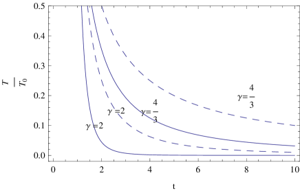
Figure 1: shows the plot of $\frac{T}{T_{0}}$ vs $t$ for a different value of $\gamma$ with $D=\frac{3}{2}$. Here the solid line represent the variation in the absence of viscosity while the dashing line represent that in the presence of viscosity.

It is also evident that the temperature of the universe is higher for lower values of $\gamma$ at a given instant of time.

(ii) For $s=\frac{3}{4}$, $m=\frac{5}{6}$, $\alpha\neq 0$ and $D\neq\frac{4}{3\gamma}$, the temperature of the universe evolves as $T=T_{0}t^{(3D-4-\frac{6\rho_{0}\rho_{2}D}{\Pi_{2}}+\frac{2\rho_{0}^{\frac{1}{4}}}{\beta\rho_{2}})}\left[\Pi_{0}t^{2}+\Pi_{2}\right]^{(2-\frac{3\rho_{0}D}{\Pi_{0}}+\frac{3\rho_{0}\rho_{2}D}{\Pi_{2}})}\left[t^{2}+\rho_{2}\right]^{-6-\frac{\rho_{0}^{\frac{1}{4}}}{\beta\rho_{2}}}$. At the later stage of evolution of the universe ($t>>\Pi_{2}$ and $t>>\rho_{2}$) one can obtain the power law variation of temperature. Using Gibbs integrability condition the temperature evolution of the universe becomes $T=T_{0}t^{\frac{-12(\gamma-1)}{\gamma}}$. Here the condition $D>\frac{4}{\gamma}$ ensure the negative value of bulk viscous stress.

(iii) For $s=\frac{m+1}{2}$, the temperature of the universe in GR ($\alpha=0$) may be evaluated using Gibbs integrability condition (15) and eq. (9), we obtain the following variation of temperature :

$$T=T_{0}t^{\frac{-2(\gamma-1)}{\gamma(1-m)}},$$ (25)

which is decaying if $\gamma>1$, $m<1$ or $\gamma<1$, $m>1$. Here the negative value of bulk viscous stress ($\Pi$) is obtain for $\Pi_{0}>0$ ( i. e., $D>\frac{4}{3\gamma(1-m)}$). The condition $D>\frac{4}{3\gamma(1-m)}$ also implies that in an expanding universe the temperature decrease less rapidly in the presence of viscosity compared to that when viscosity is absent. The plot of $T$ Vs. $t$ in fig. (2) shows that at a given time, a universe with higher temperature is possible when the cosmological constant is gradually decreased in GR. It permits a universe with late acceleration.

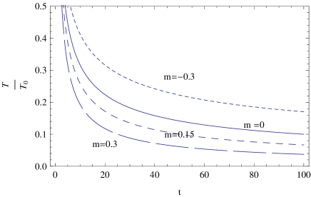
Figure 2: shows the plot of $\frac{T}{T_{0}}$ Vs. $t$ for a different value of cosmological constant (i.e., m) for $\gamma=\frac{4}{3}$.

Using the eq. (25), One can obtain the temperature of the viscous universe at the different epoch of cosmological evolutions of the universe. To obtain the temperature at present epoch we set the initial condition $T_{0}=1\times 10^{10}$ at $t=1$ [26] i.e., during the cosmological epoch of decoupling of neutrinos from the cosmic plasma. Considering age of the present universe $\sim 10^{10}$ years $\sim 3.15\times 10^{17}$ second, $\gamma=\frac{4}{3}$ (radiation) and cosmological constant $\Lambda=3\times 0.085\times H^{2}(i.e.,m=0.085)$, eq. (25) leads to $T\sim 2.74$K which is in fair agreement with observed value $T\sim 2.72$K from CMBR. So, the solution admits observed value of temperature from CMBR in the presence of a small value of cosmological constant with an late accelerating universe.

3.2 Exponential models:

The set of eqs. (7), (9), (18)-(19) also admit cosmological solution with a universe without singularity . We discuss two such cases.
Case I : We note that Hubble parameter satisfying a differential equation

$$\dot{H}=\eta H-\frac{3}{2}H^{2},$$ (26)

is permitted with $\eta=\sqrt{\frac{1-m}{6\alpha}}$. This admits a ever expanding universe with no singularity, such a solution admits emergent universe scenario [27]. In this case the corresponding variation of gravitational constant and energy density are given by

$$G=G_{0}exp[bH^{-2}],$$ (27)

$$\rho=\rho_{0}H^{4}exp[-bH^{-2}],$$ (28)

where $\rho_{0}=\frac{81\alpha}{2}$ (with $8\pi G_{0}=1$) and $b=\frac{2m}{27\alpha}$ and $G_{0}=const.$ It is evident that the model admits a constant $G$ when $\Lambda=0$. The bulk viscous stress is obtained from eq. (18), which yields

$$\Pi=(2-\gamma)\rho-\frac{1}{3}\rho H^{-3}\left[4\eta H^{2}+2b\eta-3bH\right].$$ (29)

We note that without a cosmological constant ($\Lambda=0$), one obtains a realistic solution when Hubble parameter satisfies an upper bound $H<\frac{4\eta}{3(2-\gamma)}$. The temperature evolution of the universe in full causal theory is obtained from eq. (23), which yields

$$T=T_{0}\;e^{f(H)}\;e^{g(H)}\;\;\frac{\Pi^{2}}{\rho(H-\frac{2\eta}{3})^{-2}}$$ (30)

where $f(H)=\int{\frac{6\rho H}{\Pi}}dt$ and $g(H)=\frac{2}{\beta}\int{\rho^{1-s}}dt$. The above expression of the temperature also have to satisfies the Gibbs integrability condition (15). We note the following :
(i) For $s=\frac{1}{2}$, $\beta=\frac{2\sqrt{3}}{3}$, in the absence of cosmological constant and for stiff fluid the temperature of the universe evolves as $T=T_{0}H^{2}(H-\frac{2\eta}{3})^{-2}$. When $H\ll\frac{2\eta}{3}$, the evolution of temperature becomes $T\sim H^{2}$. We obtain here a decreasing mode of temperature for an exponentially expanding universe.

The scale factor of the universe is obtained on integrating eq. (26) which is given by

$$a(t)_{\pm}=\left[a_{1}\pm a_{2}\;e^{\eta t}\right]^{\frac{2}{3}}.$$ (31)

The solution ($a_{+}$) is important for building emergent universe scenario [27]. It has no singularity and the universe originated from a static state in the infinite asymptotic past ($t\rightarrow-\infty$). In this case, we note that the solution ($a(t)=a(t)_{+}$) represents a universe which begins with a finite size in the past and grows exponentially. However, initially at $t\sim 0$, the universe is matter dominated which subsequently emerges to an accelerated phase of expansion. We note that the temperature of the universe decreases in this case. The decreasing mode of temperature obtained in the FIS theory may be relevant for the later evolution which will be taken up else where for a detail scenario.
Case II : The dynamical equation admit de Sitter solution with $H=\frac{2\eta}{3}$. The scale factor of the universe evolves as $a(t)=a_{0}e^{\frac{2\eta}{3}t}$, for a sufficient inflation to solve cosmological problems, de Sitter phase should exit after an epoch $\Delta t>\frac{195}{2\eta}$. We note de Sitter phase with

$$G=const.,\;\rho=const.,\;\Lambda=const.$$ (32)

and $\zeta=const.$ and $\tau=const.$ for $m\neq 1$. In this case that bulk viscosity also remains constant throughout the inflationary phase. The temperature of the universe in this case is found to be a constant ( similar to that obtained by A. Beesham in Ref [18]) for $\beta=\frac{\gamma\;\rho^{1-s}}{(2-\gamma)\eta}$.

We also note that for $H=\frac{2}{3}\eta$ and $m=1$, one ends up with $\Lambda=const.,$ $G=const.,$ $\rho=0,$ $\zeta=0$, $\tau=0$ and $T=0$, which is not physically relevant.

4 Distance Modulus Curves :

We now probe late universe with exponential and power law expansion taking into account observational results. The distance modulus is $\mu=5\log d_{L}+25$, where the luminosity distance $d_{L}=r_{1}(1+z)\;a(t_{0})$ and $z$ represents the red shift parameter, where $1+z=\frac{a(t_{0})}{a(t_{1})}$. We determine $r_{1}$ from

$$\int\limits_{0}^{r_{1}}\frac{dr}{\sqrt{1-kr^{2}}}=\int\limits_{t_{1}}^{t_{0}}\frac{dt}{a(t)}.$$ (33)

At the late time, the scale factor becomes $a(t)\sim a_{2}e^{\frac{2\eta t}{3}}$. For exponential expansion of the flat universe, the distance modulus relation is given by

$$\mu(z)=5\log(\frac{z(1+z)}{H_{0}})+25,$$ (34)

where $H_{0}=\frac{2\eta}{3}$. For power law expansion $(a(t)\sim t^{D})$ with $k=0$, the distance modulus relation is given by

$$\mu(z)=5\log\left((\frac{D}{H_{0}})^{\frac{1}{D}}\frac{(1+z)}{D-1}((1+z)^{\frac{D-1}{D}}-1)\right)+25.$$ (35)

The observed values of $\mu(z)$ at different $z$ parameters [28] given in table 1 are employed to draw the curves corresponding to the exponential and power law expansion of the universe discussed above. The plot are shown in figs. (3) and fig. (4) which matches with observations perfectly.

Figure 3: shows the plot of $\mu$ Vs. $z$ for supernova data (dashing line) and for the exponential expansion (solid line) with $\eta=0.00038$.

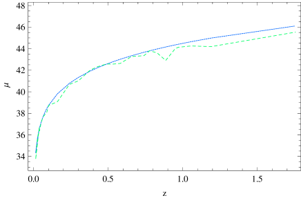
Figure 4: shows the plot of $\mu$ Vs. $z$ for supernova data (dashing line) and for the power law expansion (solid line) with $H_{0}=10^{-5}$ and $D=\frac{4}{3}$.

z	supernova $\mu$	Exponential $\mu$	Power law $\mu$
0.038	36.67	35.961	36.543
0.014	33.73	33.742	34.343
0.026	35.62	35.112	35.703
0.036	36.39	35.839	36.423
0.040	36.38	36.077	36.657
0.050	37.08	36.582	37.154
0.063	37.67	37.110	37.673
0.079	37.94	37.634	38.184
0.088	38.07	37.887	38.43
0.101	38.73	38.212	38.745
0.160	39.08	39.324	39.814
0.240	40.68	40.349	40.783
0.300	41.01	40.936	41.329
0.380	42.02	41.579	41.921
0.430	42.33	41.925	42.235
0.490	42.58	42.298	42.572
0.526	42.56	42.504	42.757
0.581	42.63	42.797	43.018
0.657	43.27	43.165	43.345
0.740	43.35	43.530	43.665
0.778	43.81	43.686	43.801
0.828	43.61	43.881	43.971
0.886	42.91	44.096	44.158
0.949	43.99	44.316	44.348
0.970	44.13	44.388	44.490
1.056	44.25	44.665	44.646
1.190	44.19	45.061	44.983
1.755	45.53	46.403	46.104

Table 1: Red shift data from Supernova, power law model and exponential model.

5 Discussions :

In this paper we study both power law and exponential behaviour of the universe with viscosity separately in a higher derivative theory of gravity considering a time varying cosmological and gravitational constant. We note that for a power law evolution of the universe, one obtains an increasing mode of gravitational constant with a positive $\Lambda$ but a decreasing mode of gravitational constant results for a negative $\Lambda$. We note a physically realistic ($\rho_{0}>0$) solution for $\Lambda<3H^{2}$. For $\Lambda=\frac{3}{2}H^{2}$ the variation of energy density ($\rho\sim t^{-4}$) is determined by $R^{2}$ term only. However, the energy density does not depend on the coupling parameter $\alpha$ in the gravitational action. We determine the characteristics temperature of a viscous universe from eq. (9), which also follows from Gibbs integrability condition. Fig. (1) shows the variation of temperature for different values of $\gamma$ in the presence or in the absence of viscosity in an accelerating universe $(q>0)$. It is evident that the higher value of $\gamma$ leads to a universe with lower temperature at a given instant of time. The evolution of temperature of a viscous universe is found to be more than that in a universe without viscosity. Fig. (2) shows the variation of temperature for different values of $\Lambda$ (determined by $m$). It is evident from fig. (2) that the rate of decrease of temperature is higher for larger values of cosmological constant in the presence of viscosity. Here we obtain a interesting solution which suggests that the present temperature of the universe is $T\sim 2.745$K, which is in fair agreement with observed value $T\sim 2.72$K from CMBR, for a radiation dominated late accelerating universe in the presence of a positive cosmological ($\Lambda=3\times 0.085\times H^{2}$) in GR. We also note cosmological solutions which admit a universe originating from singularity free state. One of the solution corresponds to emergent universe [27] which is interesting. We obtain a de Sitter solution with $\Lambda\neq 3H^{2}$. The figs. (3)-(4) show the plot of distance modulus ($\mu$) vs red shift parameter ($z$). The figures indicate that power-law and exponential model support the present observational data perfectly well.

References

- [1] S. Perlmutter , 391 (1998); S. Perlmutter , 483 (1997); A. G Riess , 1009 (1998); S. Perlmutter , 565 (1999).
- [2] D. N. Spergel , , 175 (2003); L. Page , 233 (2003); L. Verde , , 195 (2003); S. Bridel, O. Lahav, J. P. Ostriker and P. J. Steinhardt, , 1532 (2003); C. Bennet , 1 (2003).
- [3] A. G Riess , 36 (1986).
- [4] A. A. Starobinsky, , 99 (1980); L. A. Kofman, A. D. Linde and A. A. Starobinsky , 361 (1985); S. W. Hawking and J. C. Luttrell, , 250 (1984); A. Vilenkin, , 2411 (1985); M. B. Mijic, M. S. Morris and W. Suen, , 2934 (1986); B. C. Paul, D. P. Datta and S. Mukherjee, , 843 (1988); S. Gottlober and V. Muller, 183 (1986).
- [5] A. H. Guth, , 347 (1981).
- [6] A. D. Linde, , 925 (1984); R. H. Brandenberger, , 1 (1985); D. H. Lyth and D. Roberts, , 7120 (1998); L. Mersini, , 1933 (2001); A. Linde, , 89 (2002).
- [7] K. S. Stelle, , 953 (1977).
- [8] A. D. Dolgov and M. Kawasaki, , 1 (2003), S. Nojiri and S. D. Odintsov, , 123512 (2003), C. G. Bhomer, L. Hollenstein and F. S. N. Lobo , 084005 (2007); J. D. Barrow, G. F. R. Ellis, R. Maarteens, C. G. Tsagas, , 155 (2003); S. Cotsaki and G. Flessas, , 8 (1993); V. Faraoni, , 104017 (2006); I. Sawicki and W. Hu, , 127502 (2007); S. Nojiri and S. D. Odintsov, , 026007 (2008).
- [9] L. P. Chimento and A. S. Jakubi, , 71 (1995); J. D. Barrow, , 279 (1993); L. P. Chimento and A. E. Cossarini, , 1177 (1994); M. Kenmoku, K. Otsuki, K. Shigemoto and K. Uehara, , 1751 (1996).
- [10] C. W. Misner, , 431 (1968); J. D. Barrow and R. A. Matzner, , 719 (1977); B. L. Hu, in , eds. L. Z. Fang and R. Ruffini (World Scientific, Singapore, 1983).
- [11] D. Pavon and W. Zimdhal, , 261 (1993).
- [12] W. Zimdahl, D. J. Schwarz, A. B. Balakin, D. Pavon, , 063501 (2001); D. Pavon , 375 (1991); G. M. Kremer and F. P Devecchi, , 047301 (2003).
- [13] P. A. M. Dirac , 199 (1938).
- [14] P. J. E. Peebles, B. Ratra, , 559 (2003); J. D. Barrow and A. C. Ottewil, , 2757 (1983); B. Ratra and A. J. P. Peblees, , 3406 ( 1998); M. Zakari and D. Jou, , 1597 (1993); R. Maartens, , 1455 (1995); P. S. Debnath and B. C. Paul, , 189 (2006).
- [15] R. G. Vishwakarma, , 1973 (2001); R. G. Vishwakarma, , 776 (2002).
- [16] W. Chen and Y. S. Wu, , 695 (1990); W. Chen and Y. S. Wu, , 4728 (1992) [Erratum]; V. Sahni , 453 (1990); V. Sahni and A. Starobinsky, , 373 (2000); J. Garriga, A. Vilenkin, , 023517 (2001); M. Özer, M. O. Taha, , 571 (1998).
- [17] M. S. Berman and M. M. Som, , 1411 (1990); M. S. Berman and M. M. Som and F. M. Gomide, , 287 (1989); M. S. Berman, , 567 (1990); M. S. Berman, , 1419 (1990).
- [18] G.M. Kremer, F.P. Devecchi, , 047301 (2003); M. K. Mak, T. Harko, , 447 (2002); A. Beesham, , 159 (1993), Y. K. Lau and S. J. Prokhovnik , 339 (1986); V. Mendez and D. Pavon, , 679 (1996); A-M. M. Abdel-Rahman, , 3497(1992); M. K. Mark and T. Harko, , 5458 (1998); , 1171 (1998); , 273 (1999); Arbab I. Arbab and A. Beesham, , 615 (2000); A. I. Arbab, , 61 (1997); , 371 (1998).
- [19] C. Eckart, , 919 (1940).
- [20] W. A. Hiskock and L. Lindblom, , 725 (1985); W. A. Hiscock, , 1527 (1986).
- [21] I. Muller, , 329 (1967); W. A. Hiscock and J. Salmonson, , 3249 (1991);
- [22] W. Israel, , 329 (1967); W. Israel and J. M. Stewart, , 341 (1970).
- [23] D. Pavon, D. Jou and J. Casas Vazquez, , 79 (1982); D. Pavon , 375 (1991); A. M. Anile, D. Pavon and V. Romano, (1998) [gr-qc/9810014].
- [24] G. P. Singh and S. Kotambkar, , 206 (2003); B. C. Paul, Phys. Rev. D 64, 027302 (2001) ; A. Pradhan, P. Pandey, G. P. Singh and R. V. Deshpandey, Spacetime and Substance 6, 116 (2005); T. Singh and A. Beesham, , 607 (2000); P. S. Debnath, B. C. Paul and A. Beesham , 123505 (2007).
- [25] M. O. Calvao, J. A. S. Lima and I. Waga, , 223 (1992); J. A. S. Lima and A. S.M. Germano, , 373 (1992); W. Zimdahl, , 5483 (1996); G. P. Singh and A. Y. Kale, , 1177 (2009); J. A. S. Lima, A. S. M. Germano and L. R. W. Abramo, , 8 (1996).
- [26] R. Maartens, Extended Irreversible Thermodynamics in Relativity ( Hanno Rund Lectures, 1996).
- [27] S. Mukherjee, B. C. Paul, N. K. Dadhich, S. D. Maharaj and A. Beesham, Class. quantum Grav. 23 6927 (2006).
- [28] A. G. Riess, , 665 (2004).