Afterglow of binary neutron star merger

Abstract

The merger of two neutron stars results often in a rapidly and differentially rotating hypermassive neutron star (HMNS). We show by numerical-relativity simulation that the magnetic-field profile around such HMNS is dynamically varied during its subsequent evolution, and as a result, electromagnetic radiation with a large luminosity $\sim 0.1B^{2}R^{3}\Omega$ is emitted with baryon ($B$, $R$, and $\Omega$ are poloidal magnetic-field strength at stellar surface, stellar radius, and angular velocity of a HMNS). The predicted luminosity of electromagnetic radiation, which is primarily emitted along the magnetic-dipole direction, is $\sim 10^{47}(B/10^{13}~{}{\rm G})^{2}(R/10~{}{\rm km})^{3}(\Omega/10^{4}~{}{\rm rad/s})$ ergs/s, that is comparable to the luminosity of quasars.

1. Introduction

Coalescence of binary neutron stars (BNS) is one of the most promising sources for next-generation kilo-meter size gravitational-wave detectors such as advanced LIGO, advanced VIRGO, and LCGT. Statistical studies have suggested that the detection rate of gravitational waves emitted by BNS will be $\sim 1$–100 per year (Kalogera et al., 2007). Typical signal-to-noise ratio for such detection will be $\sim 10$ or less. Thus, it will be crucial for the detection of gravitational waves to find electromagnetic counterparts to the gravitational-wave signals. Short-hard gamma-ray bursts (SGRB) have been inferred to accompany with the BNS merger (Narayan et al., 1992; Piran, 2004). However, this hypothesis relies on many uncertain assumptions; e.g., high magnetic-field strength or efficient pair annihilation of neutrino-antineutrino. In this article, we give a conservative estimate for the strength of electromagnetic signals based on a numerical-relativity simulation and show that a strong electromagnetic signal will indeed accompany with the BNS merger.

BNS evolves due to gravitational radiation reaction and eventually merges. After the merger sets in, there are two possible fates (e.g., Shibata et al. (2005); Kiuchi et al. (2009)): If the total mass $M$ is larger than a critical mass $M_{c}$, a black hole will be formed, while a hypermassive neutron star (HMNS) will be formed for $M<M_{c}$. The value of $M_{c}$ depends strongly on the equation of state (EOS) of neutron stars, but the latest discovery of a high-mass neutron star with mass $1.97\pm 0.04M_{\odot}$ (Demorest et al., 2010) indicates that the EOS is stiff and $M_{c}$ may be larger than the typical total mass of the BNS $\sim 2.7M_{\odot}$ (Stairs, 2004). This indicates that HMNS is the likely outcome for many BNS mergers, at least temporarily (Hotokezaka et al., 2011).

Neutron stars in nature have a strong magnetic field with typical field strength at the stellar surface $10^{11}$–$10^{13}$ G. One of the neutron stars in BNS often has field strength smaller than this typical value as $\sim 10^{10}$–$10^{11}$ G (Lorimer, 2008), probably because of the accretion history of the first-formed neutron star during the formation of the second one. However, at least the second one is likely to have the typical magnetic-field strength.

It is reasonable to believe that each neutron star in the inspiral phase (before the merger sets in) has an approximately dipole magnetic field as in the isolated one. During the late inspiral phase and formation of a HMNS in the merger phase, its magnetic-field profile will be modified due to magnetohydrodynamics (MHD) processes. However, in zeroth approximation, it would be safe to suppose that the dipole field is dominant. Due to this reason, we consider the evolution of a HMNS with dipole magnetic fields in the following.

One of the most important properties of HMNS is that it is rapidly and differentially rotating (Shibata et al., 2005). The numerical simulations have shown that the typical angular velocity at its center is $\Omega\mathrel{\raise 1.29167pt\hbox{$>$}\mkern-14.0mu\lower 2.58334pt\hbox{$\sim$}}10^{4}$ rad/s, much larger than that of ordinary pulsars, while at equatorial surface it is $\sim 10^{3}$ rad/s. Because of the presence of the differential rotation, the winding of magnetic fields is enhanced: Toroidal magnetic-field strength $B_{T}$ in HMNS increases linearly with time ($t$) in the presence of seed poloidal (cylindrically radial) magnetic fields $B_{P}$ ($B_{T}$ increases as $\sim B_{P}\Omega t$). The increase of the magnetic-field strength results in the increase of magnetic pressure. Because only dilute matter is present in the surface of HMNS, Alfvén waves are likely to propagate near the rotational axis with $\varpi\mathrel{\raise 1.29167pt\hbox{$<$}\mkern-14.0mu\lower 2.58334pt\hbox{$\sim$}}10$ km, where $\varpi=\sqrt{x^{2}+y^{2}}$, transporting electromagnetic energy generated in HMNS along the rotational axis; tower-type outflow is driven. As far as the HMNS is alive and the rapid rotation is present, the amplification of the toroidal magnetic field continues via the winding effect. Then, the electromagnetic energy should increase approximately as $\dot{E}_{B}\sim B_{P}^{2}V\Omega$ as described in Meier (1999) where $V$ is an effective volume for which the amplification occurs. If the amplification efficiently occurs near the rotation axis with $\varpi\mathrel{\raise 1.29167pt\hbox{$<$}\mkern-14.0mu\lower 2.58334pt\hbox{$\sim$}}10$ km, $V$ is approximately $\sim(\alpha R)^{3}$ where $R$ is the equatorial stellar radius $\sim 10$ km and $\alpha$ is a constant of $O(0.1)$. For a typical HMNS formed after the merger

$$\dot{E}_{B} \sim 10^{46}B_{13}^{2}~{}R_{6}^{3}~{}\Omega_{4}\alpha_{0.1}^{3}~{}{\rm ergs/s},$$ (1)

where $B_{13}=B_{P}/10^{13}$ G, $R_{6}=R/10$ km, $\Omega_{4}=\Omega/10^{4}$ rad/s, and $\alpha_{0.1}=\alpha/0.1$. We suppose a relatively high magnetic-field strength because it is likely to be amplified by compression that occurs during the merger (Rezzolla et al., 2011). Thus, the luminosity of the electromagnetic radiation will be as high as that of quasars for a typical field strength of a progenitor neutron star $B_{P}\sim 10^{12}$ G and of a resulting HMNS $B_{P}\sim 10^{13}$ G. If a substantial fraction of this generated electromagnetic energy is converted to electromagnetic radiation (as suggested, e.g., in Nakar & Piran (2011)), the merger event may be detected by telescopes as the electromagnetic signals.

2. Numerical simulation

Motivated by the fact mentioned above, we performed MHD simulation for a HMNS in general relativity. As the initial condition, we prepare a rapidly and differentially rotating HMNS in axisymmetric equilibrium as in Shibata et al. (2006): We constructed a HMNS model with the following piecewise polytropic EOS: $P=P_{\rm cold}=K_{1}\rho^{\Gamma_{1}}$ for $\rho\leq\rho_{\rm nuc}$ and $P_{\rm cold}=K_{2}\rho^{\Gamma_{2}}$ for $\rho\geq\rho_{\rm nuc}$. Here, $P$ and $\rho$ are the pressure and rest-mass density. We set $\Gamma_{1}=1.3$, $\Gamma_{2}=2.75$, $K_{1}=5.16\times 10^{14}$ cgs, $K_{2}=K_{1}\rho_{\rm nuc}^{\Gamma_{1}-\Gamma_{2}}$, and $\rho_{\rm nuc}=1.8\times 10^{14}~{}{\rm g/cm^{3}}$. With this EOS, the maximum gravitational mass (rest mass) is $2.01M_{\odot}~{}(2.32M_{\odot})$ for spherical neutron stars and $2.27M_{\odot}~{}(2.60M_{\odot})$ for rigidly rotating neutron stars. These are similar values to those in realistic stiff EOS (e.g.,  Read et al. (2009) for a review). We prepare a HMNS with the following physical parameters: gravitational mass $M=2.65M_{\odot}$, baryon rest mass $M_{b}=2.96M_{\odot}$, maximum density $\rho_{\rm max}=9.0\times 10^{14}~{}{\rm g/cm^{3}}$, angular momentum $J=0.82GM^{2}/c$, ratio of polar to equatorial radius 0.3, central rotation period $P_{c}=0.202$ ms, and rotation period at the equatorial surface $5.4P_{c}$. Here, $G$ is the gravitational constant. The rotation law is specified in the same way as in Baumgarte et al. (2000) with the differential rotation parameter $\hat{A}=0.8$. This HMNS is similar to that found in the BNS merger simulation of Shibata et al. (2005); Kiuchi et al. (2009) performed in nuclear-theory-based EOS. In the evolution, we employ an EOS of the form $P=P_{\rm cold}+(\Gamma_{1}-1)\rho(\varepsilon-\varepsilon_{\rm cold})$ where $\varepsilon$ is the specific internal energy and $\varepsilon_{\rm cold}$ is its cold part determined from $P_{\rm cold}$.

Poloidal magnetic fields, for which the toroidal component of the vector potential has the form $A_{\varphi}=A_{0}\varpi_{0}\varpi^{2}/(r^{2}+\varpi_{0}^{2})^{3/2}$, are superimposed on this initial condition. The magnetic field in the inertial frame is given by $B^{i}=\epsilon^{ijk}\partial_{j}A_{k}$ where $\epsilon_{ijk}$ is the completely anti-symmetric tensor. Here, $r^{2}=\varpi^{2}+z^{2}$, and $(\varpi_{0},A_{0})$ are constants: $\varpi_{0}$ is chosen to be $5R_{e}/3$–$20R_{e}/3$ where $R_{e}(=12.1~{}{\rm km})$ is the coordinate radius on the equatorial plane. We found that the electromagnetic luminosity shown below depends weakly on this parameter. In the following we show the results for $\varpi_{0}=10R_{e}/3$ and $20R_{e}/3$. $A_{0}$ determines the field strength for which we give the maximum magnetic-field strength $B_{\rm max}\approx 10^{13}$–$4\times 10^{14}$ G. Here, the magnetic-field strength is defined by $B=\sqrt{b_{\mu}b^{\mu}}$ where $b^{\mu}$ is the 4-vector of the magnetic field in the frame comoving with the fluid. With such strength, the magnetic pressure in the HMNS is much smaller than the matter pressure at its center, and thus, the density profile of the HMNS (except for its surface) is not significantly modified by the magnetic-field effect. Because of the presence of differential rotation, the magnetic fields may be amplified in the exponential manner due to the magnetorotational instability (MRI) (Balbus & Hawley, 1998). However, the wavelength for the fastest growing mode is very short ($\sim 10^{2}$–$10^{4}$ cm) in the present setting and it is not possible to resolve in numerical simulation. We here do not pay attention to the MRI but only to the winding effect. In the presence of the MRI effects, the electromagnetic energy will be increased more rapidly and the luminosity of electromagnetic radiation may be even enhanced. Thus, this work would determine the lower bound of the magnetic luminosity, that is, however, quite high.

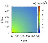
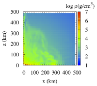
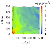
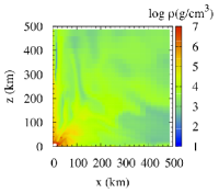
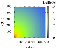
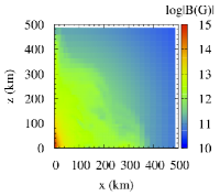
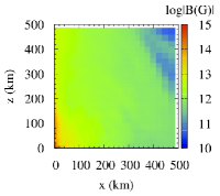
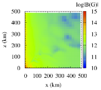
Figure 1.— Snapshots of density profiles (upper panels) and the magnetic-field strength profiles (lower panels) outside HMNS at $t=0$, 2.8, 6.2, and 12.7 ms for a model with $B_{\rm max}=1.7\times 10^{14}$ G, $\varpi_{0}=10R_{e}/3$, and $n=2$. The region with $\rho>10^{7}~{}{\rm g/cm^{3}}$ are shown to be white in the upper panels.

MHD simulation is performed assuming that ideal MHD condition holds. A conservative shock capturing scheme is employed for solving MHD equations as in Shibata & Sekiguchi (2005): In the present work, a numerical scheme with third-order accuracy in space and fourth-order accuracy in time is employed. Einstein’s evolution equations are solved in the fourth-order accuracy in space and time in the so-called BSSN-puncture formulation (Shibata & Nakamura, 1995; Baumgarte & Shapiro, 1999; Campanelli et al., 2006).

Any conservative scheme in MHD cannot handle vacuum, and hence, we have to add an atmosphere of small density outside the HMNS. Because the matter outside a HMNS formed in a real merger would be dilute, the density of the atmosphere should be as small as possible to exclude spurious effects by it. We set the density of the atmosphere as

$$\rho_{\rm at}=\Big{\{}\begin{array}[]{ll}f_{\rm at}\rho_{\rm max}&r<2R_{e},\\ f_{\rm at}\rho_{\rm max}(r/2R_{e})^{-n}&r\geq 2R_{e},\\ \end{array}$$ (4)

where we choose $n=2$ or 2.5. $f_{\rm at}$ is constant, for which we typically give $10^{-9}$. We changed the values of $f_{\rm at}$ from $10^{-10}$ to $10^{-7}$ for $B_{\rm max}=4.2\times 10^{13}$ G and found that as far as $B^{2}/(4\pi\rho_{\rm at}c^{2})\mathrel{\raise 1.29167pt\hbox{$<$}\mkern-14.0mu\lower 2.58334pt\hbox{$\sim$}}1$, our code works well. For a large value of $f_{\rm at}$, the evolution of magnetic fields is substantially affected by the inertia of the matter. However, with decreasing the value of $f_{\rm at}$ to $B^{2}/(4\pi\rho_{\rm at}c^{2})\sim 1$, the dependence of magnetic-field evolution on the atmosphere density becomes weak, and hence, the effect of the artificial atmosphere does not play a role. The velocity of the atmosphere is set to be zero initially. With this treatment, the magnetic field is initially modified for $t\mathrel{\raise 1.29167pt\hbox{$<$}\mkern-14.0mu\lower 2.58334pt\hbox{$\sim$}}P_{c}$. However, such modification plays a minor role after the winding effect becomes dominant for the magnetic field amplification. We always perform simulations for a time much longer than $P_{c}$, and focus on the stage for which a quasisteady state is achieved. Thus, the artificial effect associated with the initial setting does not matter.

Axisymmetric numerical simulation is performed in the cylindrical coordinates for MHD and in the Cartesian coordinates for Einstein’s equation part (using the so-called Cartoon method). The details are described in Shibata & Sekiguchi (2005) and its references to which the reader may refer. Nonuniform grid is prepared as in Kiuchi et al. (2008). We here impose the axial symmetry to guarantee a sufficiently high grid resolution although we can perform a nonaxisymmetric simulation. In the present setting, the equatorial coordinate radius of the HMNS, $R_{e}$, is covered by 150 uniform grids. Smaller grids with 100 and 120 were also adopted to check the convergence of the numerical results. Outer boundaries along $x$ and $z$ axes are located at $\approx 170R_{e}\approx 2000$ km.

Figure 1 plots the evolution of the density profiles and magnetic-field strength outside the HMNS. Numerical simulation shows that the system evolves in the following manner. Because of the presence of differential rotation, the winding of magnetic fields proceeds. Toroidal field strength is increased linearly with time, and the growth rate is high in particular near the rotational axis ($\varpi\mathrel{\raise 1.29167pt\hbox{$<$}\mkern-14.0mu\lower 2.58334pt\hbox{$\sim$}}10$ km). Hence, Alfvén waves propagate primarily toward $z$-direction near the rotational axis, and magnetic-field strength there also increases. After the substantial winding, the magnetic pressure $B^{2}/8\pi$ becomes larger than the gravitational potential energy density near the polar surface, $\sim GM\rho/H$ where $H(=0.3R_{e})$ is the vertical coordinate radius of the HMNS. Then, the matter of the HMNS in the vicinity of its polar surface is stripped, and an outflow is driven. Because the magnetic energy density $B^{2}/4\pi$ is comparable to or slightly smaller than the rest-mass density $\sim(H/GM)(B^{2}/8\pi)>B^{2}/4\pi c^{2}$, the outflow is mildly relativistic with the velocity of order $0.1c$ in the vicinity of the HMNS. However, in the region far from the HMNS, the outflow velocity could be fairly relativistic $\sim 0.9c$ near the rotation axis (see Fig. 3).

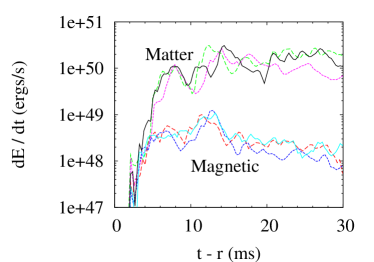
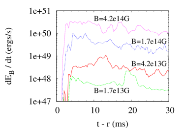
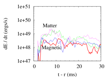
Figure 2.— Top-left: Total matter energy (upper curves) and magnetic energy (lower curves) ejection rates as functions of time for $B_{\rm max}=4.2\times 10^{13}$ G, $\varpi_{0}=10R_{e}/3$, and $n=2$. The results with three different grid resolutions are plotted: The solid, dashed, and dotted curves show the results with high, middle, and low resolutions. Top-right: The same as the top-left panel but for $(\varpi_{0},n)=(10R_{e}/3,2)$ (solid curves), $(10R_{e}/3,2.5)$ (dashed curves), and $(20R_{e}/3,2)$ (dotted curves). Bottom-left: Evolution of $\dot{E}_{B}$ for $B_{\rm max}=1.7\times 10^{13}$, $4.2\times 10^{13}$, $1.7\times 10^{14}$, and $4.2\times 10^{14}$ G. Bottom-right: The same as the top panels but for the amount integrated only for the angle $\Delta\theta=\pi/20$ radian from the rotation axis for $(\varpi_{0},n)=(10R_{e}/3,2)$ (solid curves) and $(20R_{e}/3,2)$ (dotted curves). The thick curves denote the electromagnetic luminosity. For all the figures, $r$ denotes the radius for which the surface integral of Eq. (5) is carried out.

Figure 2 plots evolution of the matter and electromagnetic energy ejection rates $\dot{E}_{M}$ and $\dot{E}_{B}$ defined by

$$\dot{E}=-\oint_{r={\rm const}}d\Omega\sqrt{-g}T^{r}_{~{}t},$$ (5)

where we substitute the stress energy tensor for the matter and electromagnetic fields into $T^{r}_{~{}~{}t}$, respectively. $g$ is the determinant of the spacetime metric. The surface integral is performed for $r\approx 480$ km. We checked that the luminosity depends only weakly on the radius of the surface integral. The top-left and top-right panels show the evolution of $\dot{E}_{M}$ and $\dot{E}_{B}$ for $B_{\rm max}=4.2\times 10^{13}$ G, and the bottom-left panel show the evolution of $\dot{E}_{B}$ for $B_{\rm max}=1.7\times 10^{13}$–$4.2\times 10^{14}$ G. The bottom-right panel shows the ejection rates integrated only for the angle $\Delta\theta=\pi/20$ for $B_{\rm max}=4.2\times 10^{13}$ G. The top-left panel is for $\varpi_{0}=10R_{e}/3$, and $n=2$ with three grid resolutions, and the top-right panel is for different values of $\varpi_{0}$ and $n$. The top-left and top-right panels show that irrespective of the grid resolution, $\varpi_{0}$, and $n$, the total ejection rates are

$$\dot{E}_{M} \sim 10^{48}B_{13}^{2}R_{6}^{3}\Omega_{4}~{}{\rm ergs/s},$$ (6)

$$\dot{E}_{B} \sim 10^{47}B_{13}^{2}R_{6}^{3}\Omega_{4}~{}{\rm ergs/s}.$$ (7)

The bottom-left panel indeed shows that the scaling relation with respect to the magnetic-field strength holds (the same scaling also holds for $\dot{E}_{M}$). Another important point is that these ejection rates do not significantly vary in time. Thus, a quasisteady outflow is driven.

The value of $\dot{E}_{B}$ agrees approximately with the prediction of Eq. (1), implying that the scenario described in Sec. 1 is correct. The ratio of $\dot{E}_{M}/\dot{E}_{B}$ is of order $2c^{2}H/GM\sim 10$. This agrees approximately with the value required for the mass stripping.

Comparison among top-left, top-right, and bottom-right panels of Fig. 2 shows that the electromagnetic energy is mainly emitted in the direction near the rotation axis. By contrast, the matter energy is emitted in a fairly isotropic manner. Along the rotational axis, $\dot{E}_{M}/\dot{E}_{B}$ is of order unity ($\sim 1$–10). This is the reason that the outflow along the rotation axis can be mildly relativistic.

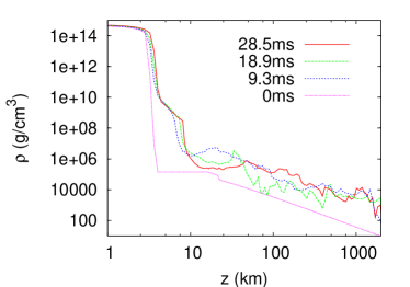
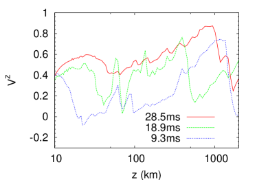
Figure 3.— Snapshots of density (left panel) and velocity profiles (right panel) along the rotation axis for $B_{\rm max}=4.2\times 10^{13}$ G, $\varpi_{0}=10R_{e}/3$, and $n=2$. At $t=0$, the density is determined by the atmosphere and decreases in the form $\rho\propto r^{-2}$ for the large radius.

The amount of angular momentum loss by the matter ejection and electromagnetic radiation in the time duration $\Delta t=P_{c}$ is much smaller than the total angular momentum because of our choice of magnetic-field strength $\mathrel{\raise 1.29167pt\hbox{$<$}\mkern-14.0mu\lower 2.58334pt\hbox{$\sim$}}3\times 10^{14}$ G. This implies that the matter and electromagnetic waves are continuously ejected, and a quasisteady outflow is formed. Figure 3 plots the density and velocity profiles along the rotation axis for $B_{\rm max}=4.2\times 10^{13}$ G, $\varpi_{0}=10R_{e}/3$, and $n=2$. The density profile (left panel) indeed shows that the averaged density does not change significantly with time. The density decreases with the radius. In these examples, the power-law index is roughly $n_{\rho}\sim 1.5$–2 ($\rho\propto r^{-n_{\rho}}$), but this number depends on the initial setting for $B_{\rm max}$ and $\varpi_{0}$ and varies with time. The velocity profile (right panel of Fig. 3) shows that the outflow is mildly relativistic. The profile varies in a short time scale. The maximum velocity is $\sim 0.9c$ as mentioned above: This maximum depends weakly on the setting of the atmosphere; for the lower atmosphere density, the maximum speed is larger. The averaged magnitude of the outflow velocity in time is $\sim 0.4$–$0.6c$ (which also depends weakly on the setting of the atmosphere). Because the corresponding Lorentz factor of the jet is $\Gamma_{j}\lesssim 2$, the relativistic beaming effect (i.e., observable viewing angle is $\lesssim 1/\Gamma_{j}$) is relatively small, and thus, this jet may be observable from a large solid angle.

3. Discussion

The centrifugal force due to rapid and differential rotation plays a crucial role for supporting strong self-gravity of HMNS. This suggests that any HMNS will eventually collapse to a black hole after a substantial loss of angular momentum by gravitational-wave emission (Shibata et al., 2005) and/or after a substantial angular momentum transport inside it due to magnetic viscous effects (Duez et al., 2006) in a realistic situation. The predicted lifetime is of order 10–100 ms. After the collapse to a black hole, a system composed of a black hole and compact accretion disk will be formed (Shibata et al., 2006; Duez et al., 2006; Rezzolla et al., 2011; Hotokezaka et al., 2011). Then, the electromagnetic radiation is likely to be emitted through the Blandford-Znajek mechanism (Blandford & Znajek, 1977; McKinney & Gammie, 2004; McKinney, 2005). However, the lifetime of the accretion disk will not be longer than $\sim 100$ ms because of the viscous evolution. Hence, the magnetic energy generation and mass ejection are likely to continue only for a short time scale of order 100 ms after the BNS merger.

However, the luminosity is quite high. If the kinetic energy of the matter and/or electromagnetic energy are efficiently converted to an electromagnetic signal, it will be observed even if the merger happens at a distance of several hundred Mpc as discussed, e.g., in Nakar & Piran (2011). Strong radio afterglow emission could be expected when the jet propagates in the matter that may be ejected from neutron stars and HMNS during the merger. The ejected mass that can be estimated as $\dot{E}_{M}\Delta T/c^{2}\sim 10^{-6}M_{\odot}B_{13}^{2}R_{6}^{3}\Omega_{4}(\Delta T/0.1~{}{\rm s})$ could yield radioactive elements and be observed like dim supernovae (Li & Paczyński, 1998).

In this article, we focus only on the HMNS with conservative magnetic field strength $B\sim 10^{13}$ G (achieved by compression of ordinary field strength $\sim 10^{12}$ G). If the magnetic field strength were as high as that of magnetar (Woods & Thompson, 2006), i.e., $B\sim 10^{15}$ G, the electromagnetic luminosity would reach $10^{51}$ ergs/s (see the bottom-left panel of Fig. 2). This value is as high as the luminosity of GRBs, and because the expected time duration is less than 1 s, this is also a candidate model for SGRB (Nakar, 2007). The canonical peak isotropic luminosity of SGRB is $\sim 10^{51}$ ergs/s, which is consistent with this estimation, assuming the jet solid angle as $\Omega_{j}\sim 0.1$ and the conversion efficiency from the jet kinetic energy into the gamma rays as $\eta\sim 0.1$. Hence, if one of neutron stars in BNS has a large magnetic-field strength or the magnetic-field strength is significantly amplified during the merger process or in the formed HMNS, this may be observed as a SGRB.

References

- Balbus & Hawley (1998) Balbus, S. A., & Hawley, J. F. 1998, Reviews of Modern Physics, 70, 1
- Baumgarte & Shapiro (1999) Baumgarte, T. W., & Shapiro, S. L. 1999, Phys. Rev. D, 59, 024007
- Baumgarte et al. (2000) Baumgarte, T. W., Shapiro, S. L., & Shibata, M. 2000, ApJ, 528, L29
- Blandford & Payne (1982) Blandford, R. D., & Payne, D. G. 1982, MNRAS, 199, 883
- Blandford & Znajek (1977) Blandford, R. D., & Znajek, R. L. 1977, MNRAS, 179, 433
- Campanelli et al. (2006) Campanelli, M., Lousto, C. O., Marronetti, P., & Zlochower, Y. 2006, Physical Review Letters, 96, 111101
- Demorest et al. (2010) Demorest, P. B., Pennucci, T., Ransom, S. M., Roberts, M. S. E., & Hessels, J. W. T. 2010, Nature, 467, 1081
- Duez et al. (2006) Duez, M. D., Liu, Y. T., Shapiro, S. L., Shibata, M., & Stephens, B. C. 2006, Phys. Rev. D, 73, 104015
- Hotokezaka et al. (2011) Hotokezaka, K., et al., submitted to Phys. Rev. D.
- Ioka & Taniguchi (2000) Ioka, K., & Taniguchi, K. 2000, ApJ, 537, 327
- Kalogera et al. (2007) Kalogera, V., Belczynski, K., Kim, C., O’Shaughnessy, R., & Willems, B. 2007, Phys. Rep., 442, 75
- Kiuchi et al. (2008) Kiuchi, K., Shibata, M., & Yoshida, S. 2008, Phys. Rev. D, 78, 024029
- Kiuchi et al. (2009) Kiuchi, K., Sekiguchi, Y., Shibata, M., & Taniguchi, K. 2009, Phys. Rev. D, 80, 064037
- Li & Paczyński (1998) Li, L.-X., & Paczyński, B. 1998, ApJ, 507, L59
- Lipunov & Panchenko (1996) Lipunov, V.M., Pancenko, I.E. 1996, A & A, 312, 937
- Lorimer (2008) Lorimer, D. R. 2008, Living Reviews in Relativity, 11, 8
- McKinney & Gammie (2004) McKinney, J. C., & Gammie, C. F. 2004, ApJ, 611, 977
- McKinney (2005) McKinney, J. C. 2005, ApJ, 630, L5
- Meier (1999) Meier, D. L. 1999, ApJ, 522, 753
- Nakar (2007) Nakar, E. 2007, Phys. Rep., 442, 166
- Nakar & Piran (2011) Nakar, E., & Piran, T. 2011, arXiv:1102.1020
- Narayan et al. (1992) Narayan, R., Paczynski, B., & Piran, T. 1992, ApJ, 395, L83
- Piran (2004) Piran, T. 2004, Reviews of Modern Physics, 76, 1143
- Read et al. (2009) Read, J. S., Lackey, B. D., Owen, B. J., & Friedman, J. L. 2009, Phys. Rev. D, 79, 124032
- Rezzolla et al. (2011) Rezzolla, L., Giacomazzo, B., Baiotti, L., Granot, J., Kouveliotou, C., & Aloy, M. A. 2011, ApJ, 732, L6
- Shapiro & Teukolsky (1983) Shapiro, S.L., & Teukolsky, S.A. 1983, Black Holes, White dwarfs, and Neutron stars, chapter 10
- Shibata & Nakamura (1995) Shibata, M., & Nakamura, T. 1995, Phys. Rev. D, 52, 5428
- Shibata et al. (2005) Shibata, M., Taniguchi, K., & Uryū, K. 2005, Phys. Rev. D, 71, 084021
- Shibata & Sekiguchi (2005) Shibata, M., & Sekiguchi, Y.-I. 2005, Phys. Rev. D, 72, 044014
- Shibata et al. (2006) Shibata, M., Duez, M. D., Liu, Y. T., Shapiro, S. L., & Stephens, B. C. 2006, Physical Review Letters, 96, 031102
- Stairs (2004) Stairs, I. H. 2004, Science, 304, 547
- Vietri (1996) Vietri, M. 1996, ApJ, 471, L95
- Woods & Thompson (2006) Woods, P. M., & Thompson, C. 2006, Compact stellar X-ray sources, 547