Data compression of measurements of peculiar velocities of Supernovae Ia

Abstract

We study the compression of information present in the correlated perturbations to the luminosity distance in the low-redshift ($z<0.1$) supernovae Ia due to peculiar velocities of these supernovae. We demonstrate that the naïve compression into angular velocity power spectrum does not work efficiently, due to thickness of the spherical shell over which the supernovae are measured. Instead, we show that measurements can be compressed into measurements of $f^{2}P(k)$, where $f$ is the logarithmic rate of growth of linear perturbations and $P(k)$ is their power spectrum. We develop an optimal quadratic estimator and show that it recovers all information for $\Lambda CDM$ models for surveys of $N\sim 10,000$ or more supernovae. We explicitly demonstrate robustness with respect to the assumed fiducial model and the number of power spectrum bins. Using mock catalogues of SNe Ia we estimate that future low redshift surveys will be able to probe $\sigma_{8}$ to $6\%$ accuracy with $10,000$ SNe Ia.

I Introduction

Since the earliest studies of supernovae, it has been suggested that type Ia (SNe Ia) might be used as standard candles for cosmological measurements. In the subsequent years many studies using SNe Ia revealed that the expansion of the universe is accelerating 1998AJ….116.1009R ; 1999ApJ…517..565P . From SNe Ia observational data one could measure cosmological parameters describing the homogeneous expansion of the universe through measurements of the luminosity distance such as matter and dark energy densities and equation of state parameters 2006A&A…447…31A ; 2007ApJ…659…98R ; 2007ApJ…666..694W ; 2002SPIE.4836…..T ; 2005AAS…20718005D ; 2006PASP..118….2H ; 2005NewAR..49..346A .

But density inhomogeneities cause additional scatter to SNe Hubble flow 1995ApJ…445L..91R ; 1997ApJ…488L…1R ; 1998ApJ…503..483Z ; 2000AAS…196.6207B ; 2004MNRAS.355.1378R ; 2006PhRvL..96s1302B ; 2007ApJ…661..650H ; 2007ApJ…659..122J ; 2007MNRAS.379..343W ; 2007ApJ…664L..13C ; 2007arXiv0705.0368W ; 2007ApJ…661L.123N ; 2008JCAP…02..022H ; 1988ApJ…332L…7G . In the recent years it has become apparent that the correlations between these peculiar velocities of the supernovae are significant at low redshifts ($z<0.1$) 2006PhRvD..73l3526H ; 2007PhRvL..99h1301G and thus present an opportunity to measure cosmological parameters that affect the growth of perturbations in the Universe such as amplitude and shape of the matter power spectrum.

But extracting any additional information from the correlations induced by peculiar-velocities comes at an expense of computing $N_{sn}\times N_{sn}$ correlation matrix and its inverse on every likelihood evaluation. To complicate matters even further, each matrix element consists of an oscillatory integrals thus adding to the cost of the overall computing time. In this paper we asses whether a data compression method can be found that will provide both efficiency and simplified form of the cosmological information carried by the peculiar velocity correlation matrix. This will also provide a physical insight into what is that the peculiar velocities of supernovae Ia are measuring.

Through the paper we assume the correlated part of peculiar velocities is described by the linear theory and that small scale virial velocities can be described by single parameter describing the velocity dispersion. While this is probably not a good approximation for realistic surveys of thousands of supernovae (after all, supernovae don’t measure velocities at random positions and the real Universe is not linear), it nevertheless provides a good simple framework for studying an efficient information compression.

The paper is structured as follows. In Section II we discuss the background theory required to describe correlations in the luminosity distances to nearby supernovae sourced by correlated large-scale velocities. In Section III we discuss the angular power spectrum of the projected velocities as a candidate for data compression. In Section IV we discuss the power spectrum multiplied by a factor describing the growth of fluctuations at mean redshift as our proposed method for data compression. We conclude in Section V.

Throughout the paper we assume that unless noted otherwise, the variables have their usual meaning.

II Correlations of peculiar velocities

The luminosity distance $d_{L}$ to a distant SN at redshift $z$ is defined by

$$F=\frac{L}{4\pi d_{L}^{2}},$$ (1)

where $F$ is the measured flux and $L$ the intrinsic luminosity of the supernovae. In the Friedmann-Robertson-Walker (FRW) metric, the luminosity distance is related to the comoving distance to an object at redshift $z$ as

$$d_{L}(z)=(1+z)\left\{\begin{array}[]{lr}\frac{1}{\sqrt{k}}\sin(\chi(z)\sqrt{k})&k>0\\ \chi(z)&k=0\\ \frac{1}{\sqrt{-k}}\sinh(\chi(z)\sqrt{-k})&k<0\end{array}\right.,$$ (2)

where $k$ is the geometrical curvature of the universe and we have introduced $\chi(z)$ as the comoving distance to a distant object at $z$ as

$$\chi(z)=\int_{0}^{z}\frac{dz^{\prime}}{H(z^{\prime})}.$$ (3)

Astronomers prefer the flux relation (Eq. (1)) rewritten in terms of the magnitudes as

$$m-M=5\log_{10}\left(\frac{d_{L}}{\mathrm{Mpc}}\right)+25,$$ (4)

where $m$ and $M$ stand for the apparent and absolute magnitude respectively.

The perturbed FRW metric leads to the effect of peculiar velocities and those in turn lead to the perturbations in luminosity distance given by 2006PhRvD..73b3523B ; 2006PhRvD..73l3526H ; 2007PhRvL..99h1301G

$$\frac{\delta d_{L}}{d_{L}}=\frac{d_{L}^{me}-d_{L}^{th}}{d_{L}^{th}}=\hat{{\bf x}}\cdot\left({\bf v}-\frac{(1+z)^{2}}{H(z)d_{L}^{th}}({\bf v}-{\bf v}_{o})\right),$$ (5)

where $d_{L}^{me}$ and $d_{L}^{th}$ stand for measured luminosity distance and theoretical prediction for unperturbed space-time, given by Eq. (2). Velocities ${\bf v}$ and ${\bf v}_{o}$ are peculiar velocities of the source and the observer respectively. Projection of peculiar velocities along the line of sight ($\hat{{\bf x}}$) is the only component we can measure. Redshift $z$ on the right-hand side of the equation stands for the observed redshift.

Since the peculiar velocities result from some initial Gaussian matter perturbations, the peculiar velocity measurements are drawn from a distribution with zero mean and nonzero variance. The later can be written in the form of correlation function as $\xi({\bf x}_{1},{\bf x}_{2})=\langle({\bf v}({\bf x}_{1})\cdot\hat{{\bf x}}_{1})({\bf v}({\bf x}_{2})\cdot\hat{{\bf x}}_{2})^{*}\rangle$ for two SN at comoving position $x_{1,2}$. The correlation function of projected peculiar velocities has been computed in a number of studies 2007PhRvL..99h1301G ; Dodelson . The result, assuming linear perturbation theory, can be written as

$$\xi({\bf x}_{1},{\bf x}_{2})= \sin{\theta_{1}}\sin{\theta_{2}}\xi_{\perp}(x,z_{1},z_{2})+$$

$$+\cos{\theta_{1}}\cos{\theta_{2}}\xi_{\parallel}(x,z_{1},z_{2}),$$ (6)

where ${\bf x}_{12}\equiv{\bf x}_{1}-{\bf x}_{2}$, $x=|{\bf x}_{12}|$, $\cos{\theta_{1}}\equiv\hat{{\bf x}}_{1}\cdot\hat{{\bf x}}_{12}$ and $\cos{\theta_{2}}\equiv\hat{{\bf x}}_{2}\cdot\hat{{\bf x}}_{12}$. The projections of the correlation function are given by 2007PhRvL..99h1301G ; Dodelson

$$\xi_{\parallel,\perp}={\bar{D}}^{\prime}(z_{1}){\bar{D}}^{\prime}(z_{2})\int_{0}^{\infty}\frac{dk}{2\pi^{2}}P(k)K_{\parallel,\perp}(kx),$$ (7)

where ${\bar{D}}(z)$ is the normalized growth function (${\bar{D}}(z)=D(z)/D(z=0)$) and derivatives are with respect to conformal time (${}^{\prime}=d/d\eta$, $a(t)d\eta=cdt$). $P(k)$ is the matter power spectrum and integration kernels are given by $K_{\parallel}(x)=j_{0}(x)-\frac{2j_{1}(x)}{x}$ and $K_{\perp}(x)=\frac{j_{1}(x)}{x}$.

Correlations in the peculiar velocity lead to correlations in the luminosity distance fluctuations which can be written as 2007PhRvL..99h1301G

$$C_{v}(i,j)=\left(1-\frac{(1+z)^{2}}{H(z)d_{L}}\right)_{i}\left(1-\frac{(1+z)^{2}}{H(z)d_{L}}\right)_{j}\xi({\bf x}_{\bf i},{\bf x}_{\bf j}).$$ (8)

The total correlation matrix is a sum of peculiar velocity correlation matrix and uncorrelated scatter $\sigma_{i}^{2}$ and can be written as 2007PhRvL..99h1301G

$$C_{ij}=C_{v}(i,j)+\delta_{ij}\sigma_{i}^{2}.$$ (9)

The diagonal parts of the matrix given by 2007PhRvL..99h1301G

$$\sigma_{i}^{2}=\left(\frac{\ln{10}}{5}\right)^{2}(\sigma_{m}^{2}+\sigma_{m_{i}}^{2})+\left(1-\frac{(1+z)^{2}}{H(z)d_{L}}\right)_{i}^{2}\sigma_{v}^{2},$$ (10)

where $\sigma_{m_{i}}$ stands for observational errors on apparent magnitudes, which are a property of the dataset and vary from supernova to supernova. The remaining two parameters are $\sigma_{m}$, which is intrinsic magnitude scatter describing deviations of supernova luminosities from the perfect standard candles, while $\sigma_{v}$ is the small scale velocity dispersion due to uncorrelated small scale peculiar velocities.

III Projected velocity angular power spectrum

Measurements of the SNe are most commonly transformed into luminosity distances or, in case of peculiar velocities, into luminosity distance fluctuations. But there is no apparent reason why not to work with the projected peculiar velocity field instead 2008JCAP…02..022H . Since we are interested in the velocity perturbations along the line of sight, the projected peculiar velocity field seems more natural as well. Those velocity perturbations can be understood as perturbations relative to the expansion of the universe in physical coordinates, or as perturbations with respect to the comoving grid.

Since the peculiar velocity field is a scalar function on a sphere, it is natural to consider its angular power spectrum. Using expansion over spherical harmonics we get

$${\bf v}(z)\cdot\hat{r}z=\sum_{\ell=0}^{\infty}\sum_{m=-\ell}^{+\ell}a_{\ell m}(z)Y_{\ell m}(\theta,\phi),$$ (11)

where we kept the dependence of the expansion on redshift $z$, i.e. we consider infinitely thin spherical shells at redshift $z$. $Y_{\ell m}$ are spherical harmonic functions that satisfy orthonormal relation

$$\int d\Omega Y_{\ell m}(\theta,\phi)Y^{*}_{\ell^{\prime}m^{\prime}}(\theta,\phi)=\delta_{\ell\ell^{\prime}}\delta_{mm^{\prime}}.$$ (12)

Using the assumption of Gaussian initial perturbations we can relate angular auto and cross power spectra to the expansion coefficients ($a_{\ell m}$) as

$$\langle a_{\ell m}(z)a^{*}_{\ell^{\prime}m^{\prime}}(z^{\prime})\rangle=C_{\ell}(z,z^{\prime})\delta_{\ell\ell^{\prime}}\delta_{mm^{\prime}}.$$ (13)

In the linear theory, these are given by

$$C_{\ell}(z,z^{\prime}) =\bar{D}^{\prime}(z)\bar{D}^{\prime}(z^{\prime})\frac{2}{\pi}\cdot$$

$$\cdot\int_{0}^{\infty}dkP(k)\left(\frac{\partial j_{\ell}(k\chi)}{\chi\partial k}\right)\left(\frac{\partial j_{\ell}(k\chi^{\prime})}{\chi^{\prime}\partial k}\right),$$ (14)

for two SNe at the redshifts $z$ and $z^{\prime}$, where $\bar{D}$ is the growth factor, $j_{\ell}$ are spherical Bessel functions, $\chi^{(^{\prime})}=\chi(z^{(^{\prime})})$ and $P(k)$ matter power spectrum. The detailed derivation can be found in the Appendix.

The angular power spectrum of luminosity distance fluctutations are exactly the same as in Eq. (14) save for the prefactors and can be written as

$$D_{\ell}(z,z^{\prime}) =\left(1-\frac{(1+z)^{2}}{H(z)d_{L}(z)}\right)\cdot$$

$$\cdot\left(1-\frac{(1+z^{\prime})^{2}}{H(z^{\prime})d_{L}(z^{\prime})}\right)C_{\ell}(z,z^{\prime}).$$ (15)

Both angular power spectra have dimensionless units. This is due to the fact that velocity in our all calculations is in the units of the speed of light.

Figure (1) shows the auto-power spectrum $D_{\ell}(z,z)$ for different values of redshift. As expected and also shown in the literature 2008JCAP…02..022H , numerical simulations are in good agreement with above result (Eq. (14)) only for small $\ell$ ($\ell<100$), where linear regime is still valid.

Figure 1: The luminosity distance fluctutations angular power spectrum plotted as $\ell(\ell+1)D_{\ell}/2\pi$ vs $\ell$ for three different redshifts: $z=0.05$ (solid), $z=0.1$ (dashed) and $z=0.01$ (dot-dashed). The angular power spectrum has dimensionless units.

Figure 2: The cross correlation coefficient $r(z)$ (Eq. 16) with respect to reference redshift $z_{m}=0.016528$. The coefficient is plotted for four low multipoles: $\ell=2$ (solid), $\ell=3$ (dashed), $\ell=4$ (dot-dashed) and $\ell=5$ (dotted).

Although the formalism is appealing, is the angular power spectrum actually a useful compression method for the low-redshift supernovae? If we want to describe all peculiar velocities of supernovae at low redshifts using a single power spectrum, the slices at different redshifts would essentially need to be describing the same velocity field. In order to check this assumption, we look at the cross-correlation coefficient given by

$$r(z,z^{\prime})=\frac{C_{\ell}^{2}(z,z^{\prime})}{C_{\ell}(z,z)C_{\ell}(z^{\prime},z^{\prime})}.$$ (16)

In Figure (2) we plot $r(z,z^{\prime})$ while fixing $z^{\prime}=0.016$, a median redshift of a typical low-z SNe dataset used in 2007ApJ…659..122J . We see that the ’correlation length’ of velocities in redshift is only about $\delta z=0.01$ and hence to describe all correlations between $z=0.0$ and $z=0.1$, we would need about 10 angular power spectra, together with a large covariance matrix that will describe not only the errors and their covariances at one redshift, but also those at neighbouring redshifts. This makes this approach clearly suboptimal and hence we turn the direct estimation of the three-dimensional power spectrum.

IV Effective power spectrum measurements

In any data compression technique, we try to put constraints on quantities that are as close to the data as possible and as independent of the underlying theoretical assumptions, while at the same time still capturing most of the information in the full dataset. Although the covariance matrix of perturbations to the luminosity distance depends on a number of cosmological dependent pre-factors, in addition to the underlying power spectrum $P(k)$, we show that, in the limit of supernovae being at sufficiently low redshifts, the data effectively measure $P(k)f^{2}$, where $f$ is the logarithmic growth rate, regardless of which fiducial cosmology one adopts.

Since the $P(k)$ is a continuous function of the wave vector $k$ we will approximate it with a stepwise function such that $P(k)=\text{const.}$ for $k_{\alpha}\leq k<k_{\alpha+1}$. With this in mind we can rewrite the parallel in perpendicular projections of correlation function of two SNe ($i$ and $j$) as

$$\xi_{\parallel}([k_{\alpha},k_{\alpha+1}))= \bar{D}^{\prime}(z_{i})\bar{D}^{\prime}(z_{j})\frac{P(k_{\alpha})}{2\pi^{2}x}\int_{k_{\alpha}x}^{k_{\alpha+1}x}K_{\parallel}(y)\,dy$$

$$= \bar{D}^{\prime}(z_{i})\bar{D}^{\prime}(z_{j})\frac{P(k_{\alpha})}{2\pi^{2}x}\cdot$$

$$\cdot\left(j_{1}(k_{\alpha+1}x)-j_{1}(k_{\alpha}x)\right),$$ (17)

$$\xi_{\perp}([k_{\alpha},k_{\alpha+1}))= \bar{D}^{\prime}(z_{i})\bar{D}^{\prime}(z_{j})\frac{P(k_{\alpha})}{2\pi^{2}x}\int_{k_{\alpha}x}^{k_{\alpha+1}x}K_{\perp}(y)\,dy$$

$$=\bar{D}^{\prime}(z_{i})\bar{D}^{\prime}(z_{j})\frac{P(k_{\alpha})}{4\pi^{2}x}\cdot$$

$$\cdot\left(\text{Si}(k_{\alpha+1}x)-\text{Si}(k_{\alpha}x)\right)-2\xi_{\parallel},$$ (18)

where $x=|{\bf x}_{ij}|$, ${\bf x}_{ij}={\bf x}_{i}-{\bf x}_{j}$ and ${\bf x}_{i}=\chi(z_{i})\hat{{\bf x}}_{i}$ (Eq. (3)), $\bar{D}(z)$ is normalized growth function and $j_{1}$ are spherical Bessel functions of the first kind. We have also defined integral sinus as $\text{Si}(x)=\int_{0}^{x}\frac{\sin{z}}{z}dz$. Eqs. (17) and (18) are valid only when $x\neq 0$. Because $x$ is the norm of the difference of two vectors to SN we will surely have examples where $x=0$ (peculiar velocity auto-correlation functions). When taking $x\rightarrow 0$ the above expressions simplify to

$$\xi_{\parallel,\perp}([k_{1},k_{2}))=\bar{D}^{\prime}(z_{i})\bar{D}^{\prime}(z_{j})\frac{P(k_{1})}{6\pi^{2}}\left(k_{2}-k_{1}\right).$$ (19)

Parameters we want to constrain from the SNe Ia data are values of matter power spectrum $P_{\alpha}$, and two uncorrelated errors $\sigma_{m}$ and $\sigma_{v}$ and so $N_{p}=N_{b}+2$. We have assumed that the absolute magnitude offset will be for all our purposes completely constrained from all supernovae data (including higher-redshift ones).

IV.1 Mock catalogues

To test our method we created several mock catalogues of SNe redshifts and their positions on the sky. For those catalogues we calculated their synthetic observational data in the form of luminosity distance fluctuations. We chose to model are synthetic data with fiducial cosmological parameters $(\Omega_{m}=0.24,h=0.7,w=-1,\Omega_{\Lambda}=1-\Omega_{m})$. We computed the covariance matrix give by Eq. (9) using reference linear matter power spectrum $P^{ref}(k)$ computed using CAMB. We computed eigenvalues $\lambda_{i}$ and eigenvectors $v_{\lambda_{i}}$ of covariance matrix and than, for each $\lambda_{i}$, draw a random number from a Gaussian distribution with $\sigma=\sqrt{\lambda_{i}}$ and add this number to the initially zero data vector in the direction of the $v_{\lambda_{i}}$. This procedure gave us at the end a data vector of luminosity distance fluctuations that was a linear combination of every eigenvector.

Uncorrelated errors of apparent magnitudes were randomly chosen from a uniform distribution between $0.05$ and $0.2$ mag. Moreover we assumed that any errors in the redshift are negligible. Uncorrelated magnitude and peculiar velocity scatter had fixed values of $\sigma_{m}=0.1\;\mathrm{mag}$ and $\sigma_{v}=300\;\mathrm{km/s}$.

IV.2 Optimal quadratic estimator

Because of the simplified form of our correlation matrix we chose the Newton iteration method for zero-finding of the derivative of probability function $L$, given by Dodelson

$$\ln{L}=-\frac{\Delta^{T}{\bf C}^{-1}\Delta}{2}-\frac{1}{2}\ln\left(\mathrm{det}\,{\bf C}\right)-\frac{N_{sn}}{2}\ln{2\pi},$$ (20)

where is $\Delta$ the data vector and ${\bf C}$ the correlation matrix given by Eq. (9). Our model depends on $a_{p}$, $p=1,\ldots,N_{p}$ parameters and is thus multidimensional. The correction to the parameters $a_{p}$ for Newton’s method is then given by Dodelson ; 1998PhRvD..57.2117B

$$\delta a_{p}=-\sum_{p^{\prime}}\left[\frac{\partial^{2}\ln{L(a)}}{\partial a_{p}\partial a_{p^{\prime}}}\right]^{-1}\frac{\partial\ln{L(a)}}{\partial a_{p^{\prime}}}.$$ (21)

The common simplification is to replace the second derivative of $\ln{L}$ with its ensemble average Dodelson ; 1998PhRvD..57.2117B

$$F_{pp^{\prime}} \equiv-\langle\frac{\partial^{2}\ln{L(a)}}{\partial a_{p}\partial a_{p^{\prime}}}\rangle$$

$$=\frac{1}{2}\mathrm{Tr}\left({\bf C}^{-1}\,{\bf C}_{,p}\,{\bf C}^{-1}\,{\bf C}_{,p^{\prime}}\right),$$ (22)

known as the Fisher matrix. When taking the ensemble average we assume that the underlying theory is correct and that the following relation is true $\langle\Delta\,\Delta^{T}\rangle={\bf C}$.

The correction to the parameter $a_{p}$ can then be written as Dodelson ; 1998PhRvD..57.2117B

$$\delta a_{p}=\frac{1}{2}\sum_{p^{\prime}}(F^{-1})_{pp^{\prime}}\,\mathrm{Tr}\left[\left(\Delta\,\Delta^{T}-{\bf C}\right)\left({\bf C}^{-1}\,{\bf C}_{,p^{\prime}}\,{\bf C}^{-1}\right)\right].$$ (23)

This method is called the optimal quadratic estimator (OQE) and is an iterative method. Although the OQE uses the Fisher matrix instead of the matrix of second derivatives, it converges to the same maximum. This is true because both matrices ($F$ and the matrix of second derivatives) are invertible and for both we are in maximum when $\delta a_{p}=0$. The only approximation comes in using the Fisher matrix to approximate the errors.

Since our parameters ($P_{\alpha},\sigma_{m},\sigma_{v}$) have physical meaning only when they are positive, we have checked this condition on every iteration step. Were they negative their values were put to zero.

IV.3 Application to synthetic data

Equation Eq. (7) tells that aside from the matter power spectrum, the peculiar velocity correlation function depends on the cosmology through the linear growth factor as well. Because we are interested in low-z SNe ($z<0.1$), where the peculiar velocity effect is still large, we are in the regime where the Hubble rate is almost constant, and equal the Hubble constant. In the limit of low-z we can rewrite luminosity distances for flat universe as

$$d_{L}\approx(1+z)\frac{cz}{H_{0}},\qquad H(t)\approx H_{0}.$$ (24)

With this in mind the factors in the luminosity distance correlation matrix (Eq. (8)) become independent of cosmological parameters. A little more care must be exercised with the derivative of the growth factor. If we expand it into a more suitable form

$${\bar{D}}^{\prime}(z)=\frac{d{\bar{D}}(z)}{d\eta}= \frac{1}{c}f(a)\,a\,H(a)\,\frac{D(z)}{D(z=0)}$$

$$= \frac{1}{c}f(a)\,\frac{1}{1+z}\,H(a)\,{\bar{D}}(z),$$ (25)

where we have defined logarithmic growth rate $f$ as

$$f\equiv\frac{a}{D(a)}\frac{dD(a)}{da}=\frac{d\ln{D}}{d\ln{a}}.$$ (26)

Therefore, in this limit we can approximate

$${\bar{D}}^{\prime}(z){\bar{D}}^{\prime}(z^{\prime})P(k)\\ \approx\frac{H_{0}^{2}}{(1+z)(1+z^{\prime})}f(z)f(z^{\prime})({\bar{D}}(z){\bar{D}}(z^{\prime})P(k))\\ \approx\frac{H_{0}^{2}}{(1+z)(1+z^{\prime})}\left(f^{2}({\bar{z}})P(k,\bar{z})\right)$$ (27)

This illustrates that in the limit of small redshifts, the relevant quantity that our method is sensitive to is a non-dimensional growth factor multiplying matter power spectrum at some effective redshift (which we show to be the mean redshift). Our final result for the correlation matrix is thus algebraic combination of Eqs. (8), (9), (17), (18), (19) and (27).

First, we have tested our method assuming a future survey of 10,000 supernovae Ia. We plot the results, together with the theoretical model used to create the dataset in Figure (3). This illustrates that the method basically works. We will proceed with a series of tests.

Figure 3: Shows the result of the new method in the form $(f^{2}P(k,z))_{\alpha}$ (datapoints with errors) and the underlying model that went into creation of synthetic dataset (solid line).

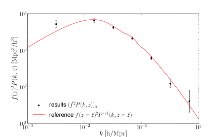
First, we have tested our method using synthetic data with different number of SN (1000,5000,10000) and different number of bins $N_{b}$ on which we estimated the matter power spectrum. We chose the bin positions by trial and error, so that the edge bin positions had very large errors and hence contained very little information. We therefore converged on the following set-up: one bin on small scales $1-10h/{\rm Mpc}$, two on large scales $10^{-4}-10^{-3}h/{\rm Mpc}$ and $10^{-3}-10^{-2}h/{\rm Mpc}$. The rest were uniformly distributed in the logarithmic scale over the interval $0.01-1h/{\rm Mpc}$. We always discard edge bins which contain essentially no information.

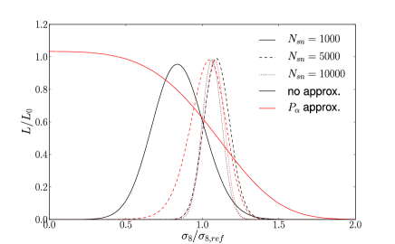
Our method relies on the overall signal-to-noise to be high enough for the central theorem limit making the power spectrum constraints have Gaussian errors. To test this, we have performed a simple test. We analysed the same synthetic data two ways. First we measured the effective power spectrum from the data and then, for a standard $\Lambda CDM$ cosmology measured the value of $\sigma_{8}$, while keeping all the other cosmological parameters fixed at their fiducial value. We then repeated the same, but this time skipped the intermediate test and measured $\sigma_{8}$ directly from the synthetic data. In the limit of infinite number of supernovae, the two should match perfectly, but we do expect deviations to appear for a small finite number of datapoints.

Results are shown in the Figure (4), where we plot the probability distributions for $\sigma_{8}$ for different number of SNe. On the vertical line we plotted the relative probability $L$. As expected, with increasing number of SNe the distributions become more alike. If we fitted Gaussian distributions we found that the variances of the distributions for $N_{sn}=5000$ differ by roughly $40\%$, while the variances for $N_{sn}=10000$ differ only by a few percent ($\sim 4\%$). We stress that the point of this exercise is to see how many supernovae are required for reaching the Gaussian limit and that in general one should marginalise over other parameters. We also note that for any given realization, the maximum likelihood is expected to be distributed around the fiducial value according to the measurement error.

Figure 4: Show the probability distribution of cosmological parameter $\sigma_{8}$ for data $P_{\alpha}$ with respect to the reference power spectrum. It shows lines representing different number of SNe at the constant number of bins $N_{b}=9$. We compare new method (red) with the brute-force calculation using Eq. (20) without approximations (black). Different line-styles represent different number of SNe: $N_{sn}=1000$ (solid), $N_{sn}=5000$ (dashed) and $N_{sn}=10000$ (dotted). $P_{\alpha}$ stands for $P_{\alpha}=(f^{2}({\bar{z}})P(k,\bar{z}))_{\alpha}$. The normalization $L_{0}$ is chosen such that $L/L_{0}$ peaks at around 1.

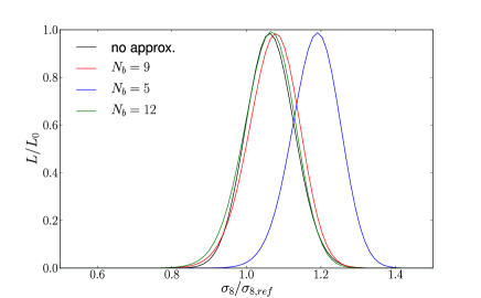
Using the same method we checked how many bins are required. We plot this in the Figure (5). The distributions vary in shape a little when changing number of bins as well as their positions in the k-space. But as long as we fix the number of bins around $N_{b}\sim 10$ the variances of the distributions vary for only a few percent.

Figure 5: Shows the probability distribution of cosmological parameter $\sigma_{8}$ for data $P_{\alpha}$ with respect to the reference power spectrum. Different line colours represent different number of bins at the constant number of SNe $N_{sn}=10000$: $N_{b}=9$ (red), $N_{b}=5$ (blue) and $N_{b}=12$ (green). Black colour represents the brute-force calculation without using any approximations. $P_{\alpha}$ stands for $P_{\alpha}=(f^{2}({\bar{z}})P(k,\bar{z}))_{\alpha}$. The normalization $L_{0}$ is chosen such that $L/L_{0}$ peaks at around 1.

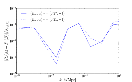
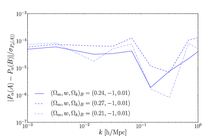
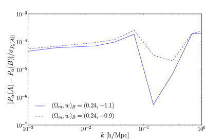
We now turn to the dependence on the assumption of the fiducial cosmological model. To this end we generate synthetic data with cosmology A ($\Omega_{m}=0.24,w=-1$) and reconstruct the matter power spectrum $P_{\alpha}$ with the same cosmology. Then we reconstruct the $P_{\alpha}$ with different cosmology $B$ ($B\neq A$) and compare the results with respect to the error on the $P_{\alpha}$ bins reconstructed with A.

Figure 6: Shows the difference of the $P_{\alpha}$ bins at different cosmologies ($A$ and $B$) with respect to the error on the result reconstructed with $A$. On the upper left plot we change $\Omega_{m}$ while keeping $w$ constant ($\Omega_{m}=0.27$ - full line, $\Omega_{m}=0.21$ - dashed; cosmology $A$ had $\Omega_{m}=0.24$). On the lower left plot we change $w$ while keeping $\Omega_{m}$ constant ($w=-1.1$ - full line, $w=-0.9$ - dashed; cosmology $A$ had $w=-1.0$). The right-hand side plots are the same as left, but we have additionally used $\Omega_{k}=0.01$ in the assumed model.

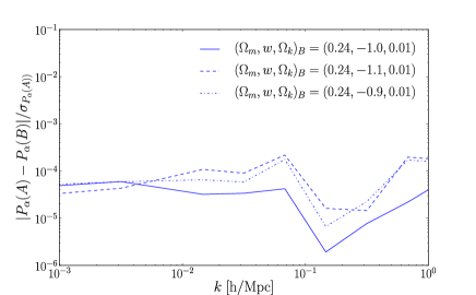Figure 6 shows that the results vary with the input cosmology only in the order of a few percent of the error and are thus negligible, when we vary parameter $\Omega_{m}$ and $w$ within their present error-bars. Which shows that even if we use the slightly wrong fiducial cosmology in the power spectrum recovery procedure, this does not affect the result significantly and that was the purpose of this new method. In this way the most cosmological information is encoded in the result ($((f\,D)^{2}P)_{\alpha}$).

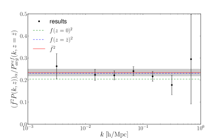
The last cross-check that we perform is to check if result can indeed be approximated as if all supernovae were at a mean redshift. The matter power spectrum and $f$ indeed vary with the redshift. In order to proceed, we divide the result of our method with average matter power spectrum for each bin ($P^{ref}_{avg}(z=\bar{z})$), where $\bar{z}$ is the mean redshift of the input SNe synthetic data. If the quantity $P^{ref}_{avg}(z=\bar{z})$ is a good estimator of what we are measuring we should get a constant line at the value of $f^{2}$. This is shown on figure (7), where we used 9 bins ($N_{b}=9$) and 10 realizations with $N_{sn}=10,000$ SNe. We see that indeed the right $f$ to use is the one evaluated at the mean redshift $f=f(z={\bar{z}})$.

Figure (4) shows that future surveys of several thousand SNe Ia will be able to estimate $\sigma_{8}$ to the accuracy of $6\%$ using $10,000$ SNe Ia.

Finally, we have investigated to what redshift we can push our method, by creating mock catalogs with increasing maximum redshfit. The approximations employed in this work clearly start to break down at z=0.2 and therefore the data need to be split into several redshift bins if working over $z=0.1$.

Figure 7: Shows the results of the new data compression method in the form $({\bar{f}}^{2}P(k,z))_{\alpha}/P^{ref}_{avg}(z=\bar{z})$ on the $k_{\alpha}$ bins. Two dashed constant lines represent values of $f$ evaluated at two different redshifts ($z=0$ - green and $z={\bar{z}}$ - blue; where $\bar{z}$ stands for the mean redshift of the synthetic SNe data). The mean of the results is shown as a full red line with $1\sigma$ errors (gray shaded region). The results are consistent with the latter ($f=f(z=\bar{z})$). We used the OQE with $N_{b}=9$ bins and 10 realizations with $N_{sn}=10,000$ SNe.

—

V Conclusions

To sum up, we presented a new data compression method for cosmological extraction of data from the low-z SNe. We have shown that these supernovae effectively measure $P(k,z)f(z)^{2}$ at the mean redshift of the supernovae survey and that in the limit of large number of supernova $N\sim 10,000$, the method is essentially optimal and unbiased. We have further shown that the correlations of supernovae velocities are sourced by perturbations on scales with wave-vectors $\sim 10^{-2}$Mpc/$h$ to $\sim 0.5$Mpc/$h$ as these scales are the most constrained.

Using mock catalogues we have shown that accuracy of $6\%$ in $\sigma_{8}$ can be obtained using $10,000$ SNe Ia with the data compression method presented in this paper. We would also like to stress that using velocity angular power spectrum should be excercised with caution, since $C_{\ell}$’s at different redshift bins are not correlated as was shown in section III. Moreover, the data compression method presented in this paper does not carry any new information, it just shows that all information is represented by $f^{2}(\bar{z})\,P(k,\bar{z})$.

These basic conclusions are unlikely to change with the real data. However, at the limit of this number of supernovae, one should worry about potential systematics and biases. Two of those are the most important. First, the actual perturbations sourcing supernovae are not in the completely linear regime any more and second, supernovae don’t trace velocity at random positions in the Universe, but instead trace it at position of rare density peaks in the primordial field, where galaxies eventually form. Corrections due to these effects can only be assessed by running $N$-body simulations. This exceeds to scope of this paper.

Recent SNe data contain of the order of a couple hundred low-redshift supernovae and so this method remains inapplicable. Unfortunately, the $10,000$ low-redshift SNe will not be available for the foreseeable future. The LSST survey predicts $\sim 100,000$ SNe per year with redshift $z<1.2$. Of this $\sim 1400$ SNe per year with $z<0.1$. However, there is no planned spectroscopic followup to these measurements. The LSST photometric redshift errors are predicted to be around $0.02(1+z)$. We examined if information on peculiar velocities could be extracted with such large redshift errors by approximating them with an extra velocity scatter of $6000$km/s, but the results are not encouraging. Photometric errors of course have an additional issue of being highly non-Gaussian.

If one could, however, measure 10,000 supernova Ia at low redshift, it might results in some interesting science. The auto-power spectrum of the population of galaxies in which supernova reside would measure the value of $P(k)b^{2}$, where $b$ is the galaxy bias, while the redshift-space distortions of the same sample would measure $\beta=f/b$. Combined with peculiar velocities measurements discussed here, one would get an over-constrained system and if analysis was done on the same volume, the sample variance would cancel out. The quantity

$$S_{G}=\frac{1}{\beta^{2}}\frac{P_{g}}{P_{sn}},$$ (28)

would therefore have a unity value in Einstein gravity and deviation from unity would indicate either new physics or systematics. Note that in using several tracers over the same field, the sample variance would cancel and thus provide a much more stringent result than one might naively guess. Similar method using weak gravitational lensing was recently used in (2010Natur.464..256R ).

—

Appendix

When computing the angular power spectrum we get

$$\langle a_{\ell m}a^{*}_{\ell^{\prime}m^{\prime}}\rangle =\bar{D}^{\prime}(z_{1})\bar{D}^{\prime}(z_{2})\int\frac{k^{2}dk}{(2\pi)^{3}}P(k)\int d\Omega_{k}\frac{1}{k^{4}}\cdot$$

$$\cdot\int d\Omega(\hat{{\bf x}}_{1})Y^{*}_{\ell m}(\hat{{\bf x}}_{1})e^{i{\bf k}\cdot{\bf x}_{1}}{\bf k}\cdot\hat{{\bf x}}_{1}\cdot$$

$$\cdot\int d\Omega(\hat{{\bf x}}_{2})Y_{\ell^{\prime}m^{\prime}}(\hat{{\bf x}}_{2})e^{-i{\bf k}\cdot{\bf x}_{2}}{\bf k}\cdot\hat{{\bf x}}_{2},$$ (A1)

where $a_{\ell m}$ stand for the expansion coefficients, $\bar{D}(z)$ is normalized linear growth factor and derivatives are with respect to conformal time ($a(t)d\eta=cdt$). In equation (A1) there are two integrals of the form

$$I_{\ell m}=\int d\Omega(\hat{{\bf x}})Y^{*}_{\ell m}(\hat{{\bf x}})e^{i{\bf k}\cdot{\bf x}}{\bf k}\cdot\hat{{\bf x}},$$ (A2)

where we have dropped the SN label in the subscript (1 or 2). We notice that the integrals in Eq. (A1) are complex conjugates, so we only need to calculate one. If we choose the coordinate system such that ${\bf k}=k\left(\sin{\theta_{k}}\cos{\phi_{k}},\sin{\theta_{k}}\sin{\phi_{k}},\cos{\theta_{k}}\right)$ and ${\bf x}=x\left(\sin{\theta}\cos{\phi},\sin{\theta}\sin{\phi},\cos{\theta}\right)$ we can rewrite the above integral into

$$I_{\ell m}=\int d\Omega Y^{*}_{\ell m}(\theta,\phi)e^{ikx\cos{\gamma}}k\cos{\gamma},$$ (A3)

where $k=|{\bf k}|$, $x=|{\bf x}|$ and $\gamma$ the angle between ${\bf k}$ in ${\bf x}$. Also the following identity is true

$$\frac{k}{ix}\frac{\partial}{\partial k}e^{ikx\cos{\gamma}}=e^{ikx\cos{\gamma}}k\cos{\gamma}.$$ (A4)

Now we are left with the integral of the exponent function over the spherical harmonics. With the use of the following mathematical identities arfken+weber

$$e^{ikr\cos{\gamma}}=\sum_{n=0}^{\infty}a_{n}j_{n}(kx)P_{n}(\cos{\gamma}),$$ (A5)

where $a_{n}=i^{n}(2n+1)$, $j_{n}$ are spherical Bessel functions and $P_{n}$ Legendre polynomials given by

$$P_{n}(\cos{\gamma})=\frac{4\pi}{2n+1}\sum_{p=-n}^{+n}Y_{np}(\theta,\phi)Y_{np}^{*}(\theta_{k},\phi_{k}),$$ (A6)

where $Y_{np}$ are spherical harmonics, we can rewrite Eq. (A3) into

$$I_{\ell m}= \frac{k}{ix}\frac{\partial}{\partial k}\sum_{n=0}^{\infty}a_{n}\frac{4\pi}{2n+1}j_{n}(kx)\cdot$$

$$\cdot\sum_{p=-n}^{+n}Y_{np}*(\theta_{k},\phi_{k})\int d\Omega Y_{\ell m}^{*}(\theta,\phi)Y_{np}(\theta,\phi),$$ (A7)

where the only integral left is the orthonormal relation of spherical harmonics

$$\int d\Omega Y_{\ell m}^{*}(\theta,\phi)Y_{np}(\theta,\phi)=\delta_{\ell n}\delta_{mp},$$ (A8)

where $\delta$’s on the right-hand side are Kronecker delta’s. Using the above identity we can evaluate both sums in the Eq. (A7) and write the result as

$$I_{\ell m} =\frac{k}{ix}\frac{\partial}{\partial k}a_{\ell}\frac{4\pi}{2\ell+1}j_{\ell}(kx)Y^{*}_{\ell m}(\theta_{k},\phi_{k})$$

$$=4\pi\,k\,i^{\ell-1}\frac{\partial j_{\ell}(kx)}{x\partial k}Y^{*}_{\ell m}(\theta_{k},\phi_{k}).$$ (A9)

Comparing the result with the original equation (A1), we have computed $I_{\ell m}(kx_{1})$. With complex conjugation and variable substitution of this result we can write the second integral as $I_{\ell^{\prime}m^{\prime}}^{*}(kx_{2})$, where $x_{1,2}=|{\bf x}_{1,2}|$. Rewriting Eq. (A1) and inserting the integral values we get

$$\langle a_{\ell m}a^{*}_{\ell^{\prime}m^{\prime}}\rangle= \bar{D}^{\prime}(z_{1})\bar{D}^{\prime}(z_{2})\int\frac{k^{2}dk}{(2\pi)^{3}}P(k)\cdot$$

$$\cdot\int d\Omega_{k}\frac{1}{k^{4}}I_{\ell m}(kx_{1})I_{\ell^{\prime}m^{\prime}}(kx_{2})$$

$$= \bar{D}^{\prime}(z_{1})\bar{D}^{\prime}(z_{2})\int\frac{2dk}{\pi}P(k)\cdot$$

$$\cdot\frac{\partial j_{\ell}(kx_{1})}{x_{1}\partial k}\frac{\partial j_{\ell^{\prime}}(kx_{2})}{x_{2}\partial k}i^{\ell-\ell^{\prime}}\cdot$$

$$\cdot\int d\Omega_{k}Y^{*}_{\ell m}(\theta_{k},\phi_{k})Y_{\ell^{\prime}m^{\prime}}(\theta_{k},\phi_{k})$$

$$= \bar{D}^{\prime}(z_{1})\bar{D}^{\prime}(z_{2})\int\frac{2dk}{\pi}P(k)\cdot$$

$$\cdot\frac{\partial j_{\ell}(kx_{1})}{x_{1}\partial k}\frac{\partial j_{\ell^{\prime}}(kx_{2})}{x_{2}\partial k}i^{\ell-\ell^{\prime}}\delta_{\ell\ell^{\prime}}\delta_{mm^{\prime}},$$ (A10)

which is exactly what we were looking for. The term on the right-hand side of the equation, that stands in front of the $\delta_{\ell\ell^{\prime}}\delta_{mm^{\prime}}$ is by definition equal to $C_{\ell}$. Implying the Kronecker delta $\delta_{\ell\ell^{\prime}}$ we can write

$$C_{\ell}(z_{1},z_{2})= \bar{D}^{\prime}(z_{1})\bar{D}^{\prime}(z_{2})\frac{2}{\pi}\cdot$$

$$\cdot\int_{0}^{\infty}dkP(k)\left(\frac{\partial j_{\ell}(kx_{1})}{x_{1}\partial k}\right)\left(\frac{\partial j_{\ell}(kx_{2})}{x_{2}\partial k}\right).$$ (A11)

References

- (1) A. G. Riess, A. V. Filippenko, P. Challis, A. Clocchiatti, A. Diercks, P. M. Garnavich, R. L. Gilliland, C. J. Hogan, S. Jha, R. P. Kirshner, B. Leibundgut, M. M. Phillips, D. Reiss, B. P. Schmidt, R. A. Schommer, R. C. Smith, J. Spyromilio, C. Stubbs, N. B. Suntzeff, and J. Tonry, AJ 116, 1009 (Sep. 1998), arXiv:astro-ph/9805201
- (2) S. Perlmutter, G. Aldering, G. Goldhaber, R. A. Knop, P. Nugent, P. G. Castro, S. Deustua, S. Fabbro, A. Goobar, D. E. Groom, I. M. Hook, A. G. Kim, M. Y. Kim, J. C. Lee, N. J. Nunes, R. Pain, C. R. Pennypacker, R. Quimby, C. Lidman, R. S. Ellis, M. Irwin, R. G. McMahon, P. Ruiz-Lapuente, N. Walton, B. Schaefer, B. J. Boyle, A. V. Filippenko, T. Matheson, A. S. Fruchter, N. Panagia, H. J. M. Newberg, W. J. Couch, and The Supernova Cosmology Project, ApJ 517, 565 (Jun. 1999), arXiv:astro-ph/9812133
- (3) P. Astier, J. Guy, N. Regnault, R. Pain, E. Aubourg, D. Balam, S. Basa, R. G. Carlberg, S. Fabbro, D. Fouchez, I. M. Hook, D. A. Howell, H. Lafoux, J. D. Neill, N. Palanque-Delabrouille, K. Perrett, C. J. Pritchet, J. Rich, M. Sullivan, R. Taillet, G. Aldering, P. Antilogus, V. Arsenijevic, C. Balland, S. Baumont, J. Bronder, H. Courtois, R. S. Ellis, M. Filiol, A. C. Gonçalves, A. Goobar, D. Guide, D. Hardin, V. Lusset, C. Lidman, R. McMahon, M. Mouchet, A. Mourao, S. Perlmutter, P. Ripoche, C. Tao, and N. Walton, A&A 447, 31 (Feb. 2006), arXiv:astro-ph/0510447
- (4) A. G. Riess, L. Strolger, S. Casertano, H. C. Ferguson, B. Mobasher, B. Gold, P. J. Challis, A. V. Filippenko, S. Jha, W. Li, J. Tonry, R. Foley, R. P. Kirshner, M. Dickinson, E. MacDonald, D. Eisenstein, M. Livio, J. Younger, C. Xu, T. Dahlén, and D. Stern, ApJ 659, 98 (Apr. 2007), arXiv:astro-ph/0611572
- (5) W. M. Wood-Vasey, G. Miknaitis, C. W. Stubbs, S. Jha, A. G. Riess, P. M. Garnavich, R. P. Kirshner, C. Aguilera, A. C. Becker, J. W. Blackman, S. Blondin, P. Challis, A. Clocchiatti, A. Conley, R. Covarrubias, T. M. Davis, A. V. Filippenko, R. J. Foley, A. Garg, M. Hicken, K. Krisciunas, B. Leibundgut, W. Li, T. Matheson, A. Miceli, G. Narayan, G. Pignata, J. L. Prieto, A. Rest, M. E. Salvo, B. P. Schmidt, R. C. Smith, J. Sollerman, J. Spyromilio, J. L. Tonry, N. B. Suntzeff, and A. Zenteno, ApJ 666, 694 (Sep. 2007), arXiv:astro-ph/0701041
- (6) J. A. Tyson and S. Wolff, eds., Society of Photo-Optical Instrumentation Engineers (SPIE) Conference Series, Presented at the Society of Photo-Optical Instrumentation Engineers (SPIE) Conference, Vol. 4836 (2002)
- (7) B. Dilday, J. Barentine, B. Bassett, A. Becker, R. Bendar, M. Bremer, H. Brewington, F. DeJongh, J. Dembicky, D. L. DePoy, M. Doi, A. Edge, E. Elson, J. Frieman, P. Garnavich, A. Goobar, T. Gueth, M. Harvanek, J. Holtzman, U. Hopp, W. Kollatschny, J. Krzesinski, D. Lamenti, H. Lampeitl, R. Kessler, B. Ketzeback, K. Konishi, D. Long, J. Marriner, J. L. Marshall, R. McMillan, J. Mendez, G. Miknaitis, R. Nichol, K. Pan, J. L. Prieto, M. Richmond, A. Riess, R. Romani, K. Romer, P. Ruiz-Lapuente, M. Sako, D. Schneider, M. Smith, S. Snedden, M. Subbarao, N. Takanashi, K. van der Heyden, C. Wheeler, and N. Yasuda, in Bulletin of the American Astronomical Society, Bulletin of the American Astronomical Society, Vol. 37 (2005) pp. 1459–+
- (8) M. Hamuy, G. Folatelli, N. I. Morrell, M. M. Phillips, N. B. Suntzeff, S. E. Persson, M. Roth, S. Gonzalez, W. Krzeminski, C. Contreras, W. L. Freedman, D. C. Murphy, B. F. Madore, P. Wyatt, J. Maza, A. V. Filippenko, W. Li, and P. A. Pinto, PASP 118, 2 (Jan. 2006), arXiv:astro-ph/0512039
- (9) G. Aldering, New Astron. Rev. 49, 346 (Nov. 2005), arXiv:astro-ph/0507426
- (10) A. G. Riess, W. H. Press, and R. P. Kirshner, ApJL 445, L91 (Jun. 1995), arXiv:astro-ph/9412017
- (11) A. G. Riess, M. Davis, J. Baker, and R. P. Kirshner, ApJL 488, L1+ (Oct. 1997), arXiv:astro-ph/9707261
- (12) I. Zehavi, A. G. Riess, R. P. Kirshner, and A. Dekel, ApJ 503, 483 (Aug. 1998), arXiv:astro-ph/9802252
- (13) A. Bonacic, R. A. Schommer, N. B. Suntzeff, and M. M. Phillips, in Bulletin of the American Astronomical Society, Bulletin of the American Astronomical Society, Vol. 32 (2000) pp. 1285–+
- (14) D. J. Radburn-Smith, J. R. Lucey, and M. J. Hudson, MNRAS 355, 1378 (Dec. 2004), arXiv:astro-ph/0409551
- (15) C. Bonvin, R. Durrer, and M. Kunz, Physical Review Letters 96, 191302 (May 2006), arXiv:astro-ph/0603240
- (16) T. Haugbølle, S. Hannestad, B. Thomsen, J. Fynbo, J. Sollerman, and S. Jha, ApJ 661, 650 (Jun. 2007), arXiv:astro-ph/0612137
- (17) S. Jha, A. G. Riess, and R. P. Kirshner, ApJ 659, 122 (Apr. 2007), arXiv:astro-ph/0612666
- (18) R. Watkins and H. A. Feldman, MNRAS 379, 343 (Jul. 2007), arXiv:astro-ph/0702751
- (19) A. Conley, R. G. Carlberg, J. Guy, D. A. Howell, S. Jha, A. G. Riess, and M. Sullivan, ApJL 664, L13 (Jul. 2007), arXiv:0705.0367
- (20) L. Wang, ArXiv e-prints(May 2007), arXiv:0705.0368
- (21) J. D. Neill, M. J. Hudson, and A. Conley, ApJL 661, L123 (Jun. 2007), arXiv:0704.1654
- (22) S. Hannestad, T. Haugbølle, and B. Thomsen, JCAP 2, 22 (Feb. 2008), arXiv:0705.0979
- (23) K. Gorski, ApJL 332, L7 (Sep. 1988)
- (24) L. Hui and P. B. Greene, Phys. Rev. D 73, 123526 (Jun. 2006), arXiv:astro-ph/0512159
- (25) C. Gordon, K. Land, and A. Slosar, Physical Review Letters 99, 081301 (Aug. 2007), arXiv:0705.1718
- (26) C. Bonvin, R. Durrer, and M. A. Gasparini, Phys. Rev. D 73, 023523 (Jan. 2006), arXiv:astro-ph/0511183
- (27) S. Dodelson, Modern Cosmology (Academic Press, 2003) ISBN ISBN-13:987-0-12-219141-1
- (28) Matter power spectrum was computed with CAMB using the following cosmological parameters ()
- (29) J. R. Bond, A. H. Jaffe, and L. Knox, Phys. Rev. D 57, 2117 (Feb. 1998), arXiv:astro-ph/9708203
- (30) R. Reyes, R. Mandelbaum, U. Seljak, T. Baldauf, J. E. Gunn, L. Lombriser, and R. E. Smith, Nature 464, 256 (Mar. 2010), arXiv:1003.2185 [astro-ph.CO]
- (31) G. B. Arfken and H. J. Weber, Mathematical Methods for Physicists, 6th ed. (Elsevier Academic Press, 2005) ISBN 0-12-088584-0