Nonequilibrium Thermodynamics of Feedback Control
Abstract
We establish a general theory of feedback control on classical stochastic thermodynamic systems, and generalize nonequilibrium equalities such as the fluctuation theorem and the Jarzynski equality in the presence of feedback control with multiple measurements. Our results are generalizations of the previous relevant works to the situations with general measurements and multi-heat baths. The obtained equalities involve additional terms that characterize the information obtained by measurements or the efficacy of feedback control. A generalized Szilard engine and a feedback-controlled ratchet are shown to satisfy the derived equalities.
pacs:
05.70.Ln,82.60.Qr,05.20.-yI Introduction
Since the mid-twentieth century, feedback control has played crucial roles in science and engineering Doyle ; Astrom . Here, “feedback” means that a control protocol depends on measurement outcomes obtained from the controlled system. Recently, feedback control has become increasingly important in terms of nonequilibrium physics, due to at least the following two reasons.
First of all, stochastic aspects of thermodynamics Sekimoto ; Bustamante ; Seifert1 have become important due to recent theoretical and experimental developments. Theoretically, a number of nonequilibrium equalities such as the fluctuation theorem and the Jarzynski equality Evans ; Gallavotti ; Jarzynski1 ; Crooks1 ; Crooks2 ; Spohn ; Maes1 ; Maes2 ; Jarzynski2 ; Kurchan ; Tasaki2 ; Hatano ; Evans2 ; Cohen ; Jarzynski3 ; Jarzynski4 ; Harada ; Seifert2 ; EspositoQ ; Gaspard ; Saito ; Ohkuma ; Kawai ; Marin ; Nakagawa1 ; Nakagawa2 ; Utsumi ; HanggiQ ; Ren ; Hasegawa ; Esposito ; HanggiQ2 ; Vaikuntanathan have recently been found. On the other hand, experimental techniques have been developed to manipulate and observe small thermodynamic systems such as macromolecules and colloidal particles, and several nonequilibrium equalities have been experimentally verified Wang ; Liphardt ; Trepagnier ; Carberry ; Collin ; Douarche ; Andrieux1 ; Toyabe1 ; Toyabe2 ; Hayashi ; Nakamura . Moreover, artificial Serreli ; Rahav ; Kay ; H and biological Schliwa molecular machines have been investigated. In these contexts, feedback control is useful to realize intended dynamical properties of small thermodynamic systems, and it has become a topic of active research Cao1 ; Kim ; Lopez ; Cao2 ; Cao3 ; Bonaldi ; Suzuki1 ; Sagawa-Ueda3 ; Suzuki2 ; Brandes ; Ponmurugan ; Horowitz ; Morikuni ; Seifert3 ; Horowitz2 ; Esposito2 ; Vaikuntanathan2 ; Sagawa ; Lahiri ; Horowitz3 ; Pekola ; Toyabe3 .
Secondly, feedback control sheds light on the foundations of thermodynamics and statistical mechanics concerning “Maxwell’s demon” Maxwell ; Demon ; Szilard ; Brillouin ; Bennett ; Landauer . In fact, Maxwell’s demon performs measurement and feedback control on thermodynamic systems. Recently, Maxwell’s demon has attracted renewed interest Lloyd1 ; Lloyd2 ; Lloyd3 ; Touchette ; Zurek ; Scully ; Kieu ; Allahverdyan ; Quan ; Nielsen ; Sagawa-Ueda1 ; Jacobs ; Sagawa-Ueda2 ; Maruyama ; SWKim from the standpoints of modern information theory and statistical mechanics.
A quintessential model of Maxwell’s demon is a single-particle heat engine proposed by L. Szilard in 1929 Szilard . During the thermodynamic cycle of the Szilard engine, the demon obtains bit ( nat) of information by a measurement, performs feedback control, and extracts of positive work from a single heat bath. After numerous arguments on the consistency between the demon and the second law of thermodynamics, it is now understood that the work needed for the demon (or equivalently the feedback controller) during the measurement and information erasure compensates for the work that can be extracted by the demon Sagawa-Ueda2 . Therefore, we cannot extract a net positive work from the total system of the engine and the demon in an isothermal cycle, and therefore the presence of the demon does not contradict the second law of thermodynamics. Nevertheless, of work extracted by the demon can be still useful. By using feedback control, we can increase the system’s free energy without injecting any energy (work) to it. We stress that, without feedback control, we need the direct energy input into the system in order to increase its free energy due to the second law of thermodynamics. Feedback control may be regarded as a powerful tool to control thermodynamic systems. Since the crucial quantity is the information that is obtained to be used for feedback control, we may regard the Szilard-type heat engine as “information heat engine.” Recently, such an information heat engine was realized experimentally by using a colloidal particle Toyabe3 .
In this paper, we formulate a general theory of feedback control on stochastic thermodynamic systems. In particular, we extend recent theoretical results on the generalizations of the fluctuation theorem and the Jarzynski equality Sagawa-Ueda3 to the situations in which the measurement and feedback control are non-Markovian and there are multi-heat baths. Our results serve as the fundamental building blocks of information heat engines.
This paper is organized as follows.
In Sec. II, we briefly review the framework of stochastic thermodynamics in a general setup. We discuss classical stochastic systems that are in general non-Markovian and in contact with multi-heat baths. We discuss the concept of entropy production and the detailed fluctuation theorem as our starting point. Because they are general properties of nonequilibrium systems, our formulations and results in the following sections are not restricted to Langevin systems but applicable to any classical stochastic systems that satisfy the detailed fluctuation theorem.
In Sec. III, we formulate measurements on thermodynamic systems. We discuss multi-measurements including continuous measurements, and investigate the properties of the mutual information obtained by the measurements. In particular, we introduce the two kinds of mutual information and , which will be shown to play key roles in the discussion of feedback control.
In Sec. IV, we discuss feedback control on Markov and non-Markov processes, and investigate feedback control in terms of probability theory, where the causality of the measurement and feedback play a crucial role.
In Sec. V, we derive the main results of this paper. We generalize the nonequilibrium equalities to situations in which the system is subject to feedback control. In particular, we derive two types of generalizations of the fluctuation theorem and the Jarzynski equality. One involves a term concerning the mutual information, and the other involves a term of feedback efficacy. As corollaries, we derive the generalizations of the second law of thermodynamics and a fluctuation-dissipation relation.
In Sec. VI, we illustrate our general results by two examples: a generalized Szilard engine with measurement errors and a feedback-controlled ratchet Cao1 ; Lopez ; Cao3 . We discuss the former analytically and the latter numerically.
In Sec. VII, we conclude this paper.
In Appendix A, we discuss the physical meaning of entropy production to elucidate the physical contents of our results in two typical situations.
II Review of Stochastic thermodynamics
In this section, we briefly review thermodynamics of classical stochastic systems and introduce notations that will be used later.
II.1 Dynamics
We consider a classical stochastic system S that is in contact with heat baths , , , at respective temperatures , , , . Let be the phase-space point of system S and be a set of external parameters such as the volume of a gas or the frequency of an optical tweezers. We control the system from time to with control protocol . Let be a trajectory of the system.
To formulate the stochastic dynamics, we discretize the time interval by dividing it into small intervals with width . The original continuous-time dynamics is recovered by taking the limit of or equivalently . Let and . We refer to “time ” as “time .” Then, trajectory corresponds to .
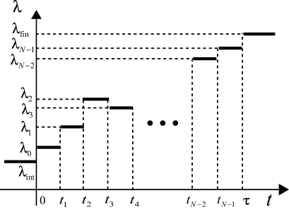
Control protocol can also be discretized. Let be the value of between and , where it is assumed to be constant during this time interval (see FIG. 1). We denote the trajectory of from time to as . Let be the value of parameter before time , which is not necessarily equal to because we can switch the value of the parameter at time . We also denote the value of after time as , which is not necessarily equal to , either (see also FIG. 1).
Let be the probability distribution of at time . In particular, is the initial distribution of . The initial distribution can be chosen as a stationary distribution under external parameters , as , which means . We note that is not necessarily a canonical distribution; it can be a nonequilibrium stationary distribution. Due to the causality, is determined by through the transition probability , which depends on the external parameters at time (i.e., ). We note that represents the the probability of realizing at time under the condition that the trajectory of up to time is given by . If the dynamics is Markovian, can be replaced by .
The probability of trajectory is then given by
| (1) |
where we write just as for simplicity. We note that
| (2) |
is the probability of trajectory under the condition that the initial state is and the control protocol is .
Let be an arbitrary physical quantity that can depend on the trajectory and protocol . The ensemble average of this quantity is given by
| (3) |
where .
II.2 Backward Control
Before proceeding to the nonequilibrium equalities, we consider the stochastic dynamics with a backward control protocol. The backward control protocol means the time-reversal of protocol , which is formulated as follows. Let be the time-reversal of ; for example, if is a magnetic field, then . The time-reversed protocol of is then given by . The backward protocol can be discretized as . We define , , and .
We consider the probability of realizing trajectory of the system with a backward control protocol. We define and . We denote as the initial distribution of the backward processes. We stress that is not necessarily equal to the final distribution of the forward experiments. In fact, we can prepare a new state for the system to perform the backward experiments after the forward experiments. The probability distribution of trajectory with backward protocol is given by
| (4) |
where we write as for simplicity. Correspondingly,
| (5) |
In special cases, the backward trajectory is equal to the time-reversal of the forward trajectory . Let be the time-reversal of phase-space point . For example, if with and being the position and the momentum respectively, we have . The time-reversal of trajectory is then given by . With notation , we write . By substituting to Eqs. (4) and (5), we obtain the probability of realizing a backward trajectory under the backward protocol as
| (6) |
where the conditional probability under initial is given by
| (7) |
We note that holds, because .
II.3 Nonequilibrium Equalities
We now discuss nonequilibrium equalities. Let be the heat that is absorbed by the system from the th heat bath satisfying . We write simply as for simplicity. It has been established that the following equality is satisfied for stochastic thermodynamic systems Crooks1 ; Crooks2 ; Jarzynski2 ; Seifert2 :
| (8) |
which is referred to as the detailed fluctuation theorem (or the transient fluctuation theorem). This is the starting point of our research. We can rewrite Eq. (8) as
| (9) |
where
| (10) |
which is called the entropy production along trajectory .
Various proofs of the detailed fluctuation theorem [Eqs. (8) and (9)] for stochastic systems have been presented, for example, in Refs. Crooks1 ; Crooks2 ; Seifert2 for the Markovian stochastic dynamics and in Ref. Ohkuma for non-Markovian Langevin systems. A proof of Eqs. (8) and (9) has also been given in Ref. Jarzynski2 for the situations in which the total system including heat baths is treated as a Hamiltonian system and the initial states of the heat baths in the forward and backward processes are the canonical distributions. This proof can confirm the physical validity of the detailed fluctuation theorem even for the non-Markovian dynamics with multi-heat baths, as the stochastic dynamics can be reproduced as that of a partial system of the total Hamiltonian system including the heat baths. We also note that several equalities that are similar but not equivalent to Eqs. (8) and (9) have been derived for different situations. For example, the transient fluctuation theorem has been discussed for dynamical systems in Ref. Evans2 . The fluctuation theorem for nonequilibrium steady states has been discussed for stochastic systems Kurchan0 ; Spohn and dynamical systems Evans ; Gallavotti .
From the detailed fluctuation theorem (9), we can show Crooks’ fluctuation theorem as follows. We denote as the probability of finding the entropy production in the forward processes, satisfying
| (11) |
where is the delta function. On the other hand, let be the probability of obtaining in the backward processes, satisfying
| (12) |
By using the detailed fluctuation theorem (9) and equality , we obtain Crooks’ fluctuation theorem
| (13) |
The detailed fluctuation theorem (9) or Crooks’ fluctuation theorem (13) leads to the integral fluctuation theorem
| (14) |
where the ensemble average is taken over all trajectories under forward protocol (see Eq. (3)). From the concavity of the exponential function, we obtain
| (15) |
which is an expression of the second law of thermodynamics: the ensemble-averaged entropy production is non-negative. By taking the ensemble average of the logarithm of both sides of Eq. (9), we have
| (16) |
which we will refer to as the Kawai-Parrondo-Broeck (KPB) equality Kawai ; Marin . The right-hand side of Eq. (16) is the Kullback-Leibler divergence (or the relative entropy) of and , which is always positive. Therefore, Eq. (16) reproduces inequality (15).
If the probability distribution of is Gaussian, the cumulant expansion of Eq. (3) leads to a variant of fluctuation-dissipation relation
| (17) |
which indicates that is determined by the fluctuation of . Equality (17) is an expression of the fluctuation-dissipation theorem of the first kind, which gives a special case of the Green-Kubo formula Evans2 .
In the case of an isothermal process with a single heat bath, the entropy production reduces to
| (18) |
where is the work performed on the system during the process, and is the difference of the free energies for the initial and final Hamiltonians (see also Appendix A for details). Under this situation, Eq. (14) leads to
| (19) |
which is the Jarzynski equality Jarzynski1 . The second law of thermodynamics then reduces to
| (20) |
III Measurement
In this section, we formulate and investigate the effect of measurements on nonequilibrium dynamics.
III.1 Classical Measurement and Mutual Information
In this subsection, we review the general framework of a measurement on a probabilistic variable, which can be applied to a broad class of measurements on classical systems.
Let be an arbitrary probability variable of a measured system whose distribution is . We perform a measurement on it and obtain outcome which is also a probability variable. The error of the measurement can be characterized by a conditional probability , which describes the probability of obtaining outcome under the condition that the true value of the measured system is . We note that for all , where we note that the sum should be replaced by the integral if is a continuous variable. If the measurement is error-free, is given by the delta function or the Kronecker’s delta. We assume that is independent of the probability distribution ; in other words, the error is independent of the state preparation of the measured system. The joint probability of and is given by , and the probability of obtaining by . The probability of realizing under the condition that the measurement outcome is , denoted as , is given by the Bayes theorem:
| (21) |
We next discuss the information contents related to the measurement Shannon ; Cover-Thomas . The Shannon information contents of the probability variables are given by
| (22) |
which characterize the randomnesses of and , respectively. On the other hand, the mutual information content between and is given by
| (23) |
where
| (24) |
In this paper, we also call the mutual information. We note that holds due to the Bayes theorem (21).
The mutual information measures the amount of information obtained by the measurement. It is known that
| (25) |
If the measurement is error-free, holds.
III.2 Measurements on Nonequilibrium Dynamics
We next formulate multiple measurements on nonequilibrium dynamics, and discuss the properties of the mutual information obtained by the measurements.
Let be the outcome at time . In this section, we assume the followings:
-
1.
The error of the measurement at time is characterizes by , where can depend on the trajectory of the system before due to the causality. Here we assumed that the property of the measurement error at time does not explicitly depend on or . This assumption is also justified in many real experimental situations.
-
2.
The unconditional probability distribution of , , is not affected by the back-action of the measurement. Since the system is classical, this assumption is justified for many real systems such as colloidal particles and macromolecules.
If , we call the measurement Markovian, which means that the outcome is determined only by the system’s state immediately before the measurement. This condition is satisfied if the measurements can be performed in a time interval that is sufficiently shorter than the shortest time scale of the system. We note that the Markovness of the measurement is independent of that of the dynamics.
We assume that the measurements are performed at times , , , , where . If , , , , hold, the measurement is time-continuous in the limit of , because the measurements are performed at all times.
We write as the set of measurement outcomes that are obtained up to time , i.e. where is the maximum satisfying . If the measurement is continuous, then .
We define
| (26) |
where is the maximum integer satisfying . Without feedback, Eq. (26) defines the conditional probability of obtaining outcomes under the condition of , while, with feedback, this interpretation of Eq. (26) is not necessarily correct as shown in the next section. To explicitly demonstrate this point and to distinguish from the usual conditional probability, we put suffix “c”. Then, the joint distribution of and is given by
| (27) |
The probability of obtaining outcomes is given by
| (28) |
where the two equalities are just identities known in probability theory. We also note that
| (29) |
which is, in fact, independent of .
We then discuss the mutual information obtained by multiple measurements on nonequilibrium dynamics. Suppose that we obtain measurement outcomes at time . If we perform another measurement at time and obtain outcome , we obtain the mutual information between and under the condition that we have obtained :
| (30) |
where we used Eq. (29). We note that, if the measurement is Markovian, reduces to . We denote as the sum of these mutual information contents obtained by multi-measurements, that is,
| (31) |
where we used Eq. (28). We note that the same quantity has been discussed in Ref. Cao2 . From Eq. (31), we find that equals the mutual information between trajectories and defined as . In the presence of feedback control, however, this is not true (i.e., ), as we will see later.
IV Feedback Control
In this section, we formulate feedback control on nonequilibrium dynamics.
IV.1 Formulation
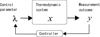
Feedback control implies that protocol depends on measurement outcomes (see FIG. 2). On the other hand, without feedback control, control protocols are predetermined and independent of the measurement outcomes, as is the case for the setup of the original fluctuation theorem and Jarzynski equality.
When the system is subject to feedback control, can depend on measurement outcomes that are obtained until , while cannot depend on any measurement outcome that is obtained after time due to causality. We introduce notation , which means that the value of at time is determined by . We write .
If only depends on as , the feedback protocol is called Markovian. We note that the Markovness of feedback is independent of that of the dynamics or measurements. The Markovian feedback control is realized when the delay time of feedback is sufficiently smaller than the smallest time scale of the dynamics.
IV.2 Overdamped Langevin System
As a simple illustrative example, we discuss an overdamped Langevin system, whose equation of motion is given by
| (32) |
where is the friction constant, is an external potential, is an external nonconservative force, and is the Gaussian white noise satisfying . The detailed fluctuation theorem (8) is still satisfied in the presence of a nonconservative force that violates the detailed balance, because Eq. (8) can be derived from the local transition rate of the stochastic dynamics and is independent whether there is a global potential or not. We assume that the measurement is time-continuous and Markovian:
| (33) |
where is a white Gaussian noise with (). The conditional probability of obtaining outcome is given by
| (34) |
The feedback protocol can be written as in general. The work performed on the system is then given by
| (35) |
where
| (36) |
In particular, if the feedback is Markovian, is given by . Then, can be written as
| (37) |
where . The first term on the right-hand side of Eq. (37) arises from a change in by the pre-fixed protocol, while the second and third terms are induced by the feedback control.
We next consider the Kalman filter and the optimal control. As a special case of Eq. (32), we consider a discretized linear Langevin equation in the Itô form:
| (38) |
where is a positive constant and is a control parameter. If the initial distribution of is Gaussian, the distribution of remains Gaussian with Eq. (38). In this case, the obtained mutual information by measurement (33) at time is given by
| (39) |
where . Therefore, the total mutual information
| (40) |
can converge, while the measurement is continuous.
We consider the Kalman filter on Eq. (38) with measurement (33). The Kalman filter is a standard method to construct the optimal estimator of , denoted as , in terms of the mean square error. From measurement outcomes , is obtained as the solution to the following simultaneous differential equations Welch :
| (41) |
| (42) |
where is a time-dependent real number and Eq. (42) is a discretized version of the Riccati equation. By using the Kalman estimator , the optimal control protocol Bertsekas is given by
| (43) |
where is a pre-determined constant depending on the target of the optimal control. We note that the optimal control is a non-Markovian control as , because we use all of to calculate . The generalized Jarzynski equality for this situation has been discussed in Ref. Suzuki2 .
IV.3 Probability Distributions with Feedback
We discuss the probability distributions with feedback control in general. Under the condition that we fix control protocol with being fixed, the conditional probability of realizing is given by
| (44) |
which corresponds to Eq. (1). We note that, in the expression in Eq. (44), we do not omit the notation because its -dependence is crucial. We also write
| (45) |
On the other hand, along the trajectory , the conditional probability of obtaining outcome at time is written as . We then define
| (46) |
which is to be compared with Eq. (26).
We then obtain the joint probability distribution of and with feedback control as
| (47) |
We can check that
| (48) |
by integrating and in Eq. (47) in the order of , where the causality of measurements and feedback play crucial roles.
The marginal distributions are given by
| (49) |
and the conditional distributions by
| (50) |
We stress that, in the presence of feedback control,
| (51) |
in general, because protocol depends on . On the other hand, without feedback control, holds because is simply given by with being independent of .
The ensemble average of a probability variable is given by
| (52) |
and the conditional average under the condition of is given by
| (53) |
Equation (29) still holds in the presence of feedback control:
| (54) |
We note that Eq. (28) also holds with feedback control.
We then define the mutual information in the same way as in the case without feedback control:
| (55) |
In the presence of feedback control, does not equal the mutual information between trajectories and defined as , because . Intuitively speaking, only characterizes the correlation between and due to the measurements, while involves the correlation due to the feedback control. Note that is a more important quantity than , because has a clear information-theoretic significance: is the information that we obtain by measurements. We also note that, in the case of a single measurement and feedback, always holds.
We also note that an identity similar to the integral fluctuation theorem holds for :
| (56) |
because
| (57) |
IV.4 Detailed Fluctuation Theorem for a Fixed Control Protocol
If we fix control protocol with being fixed, then the detailed fluctuation theorem (8) still holds:
| (58) |
where
| (59) |
The left-hand side of Eq. (58) corresponds to the following forward and backward experiments. We first perform forward experiments many times with feedback control, and choose the subensemble in which the measurement outcomes are given by . Within this subensemble, the ratio of trajectory is given by under the condition of initial . We next perform backward experiments with protocol , where was chosen in the forward experiments. We stress that we do not perform any feedback in the backward experiments: is just the time-reversal of . We then obtain as the ratio of trajectory , under the condition of initial in the backward experiments. The original detailed fluctuation theorem (8) can straightforwardly be applied to this subensemble corresponding to because we have a unique control protocol in the subensemble, and therefore we obtain Eq. (58).
Let the initial distribution of the backward experiments be which in general depends on the measurement outcomes in the forward experiments. A natural choice of is a stationary state . Then we have
| (60) |
where
| (61) |
If there is a single heat bath and the initial distributions of the forward and backward experiments are given by the canonical distributions, then the entropy production reduces to
| (62) |
where the free-energy difference can depend on the measurement outcomes as .
We list our notations in Table I.
| Phase-space point of the system. | |
|---|---|
| Time-reversal of . | |
| Discretization of time. | |
| Phase-space point at time . | |
| Trajectory of the phase-space point from time to , i.e. . | |
| Time-reversal of , i.e. with . | |
| Controllable external parameters at time . | |
| Control protocol from time to . | |
| Backward control protocol of , i.e. with . | |
| Entropy production. | |
| Measurement outcome at time . | |
| Measurement outcomes from time to . | |
| Time-reversal of , i.e. with . | |
| Protocol of feedback control with outcomes . | |
| Probability of trajectory under the condition that the protocol is given by with being fixed outcomes. | |
| Time-reversal of : | |
| Probability density of obtaining under the condition of , which characterizes the measurement error. | |
| . | |
| Joint distribution of and which is given by . | |
| Conditional mutual information obtained at time under the condition that we have outcomes . | |
| Sum of the conditional mutual information: . |
V Nonequilibrium Equalities with Feedback Control
We now discuss the main results of this paper. We derive the two types of the generalized nonequilibrium equalities with feedback control in Sec. V A and V B, respectively. The former generalization involves the mutual information, while the latter involves the efficacy of feedback control.
V.1 Generalized Fluctuation Theorem with Mutual Information
To derive a generalized detailed fluctuation theorem, we first formulate the relevant backward probabilities. We consider the following type of “backward probability distribution”:
| (63) |
which satisfies
| (64) |
Definition (63) has a clear operational meaning. Suppose that we perform a forward experiment with feedback and obtain outcome . We then perform a backward experiment with protocol . We repeat this set of the forward and backward experiments many times, and calculate the fractions of and , which respectively give and .
Noting Eq. (47) and the definition of the mutual information (55), we obtain a generalized detailed fluctuation theorem with feedback control:
| (65) |
where the effect of feedback control is involved by the term of the mutual information that is obtained in the forward experiments. We stress that, to obtain Eq. (65), we do not perform feedback control in the backward experiments. We just reverse forward protocol as Eq. (59) in the backward experiments. The same result for a special case was obtained in Ref. Horowitz . The investigation of the detailed fluctuation theorem in the situations in which feedback control is also performed in the backward processes Ponmurugan is an interesting future challenge. Such situations would be relevant to, for example, autonomous systems consisting of the controlled system and the controller, in which feedback control should also be needed for the backward processes. We can expect that the backward processes with feedback control can be used to characterize the reversibility of the autonomous systems.
From the generalized detailed fluctuation theorem (65), we obtain a generalized integral fluctuation theorem Sagawa-Ueda3 :
| (66) |
Due to the concavity of the exponential function, we obtain a generalized second law of thermodynamics Sagawa-Ueda1 ; Sagawa-Ueda3 :
| (67) |
which means that the entropy production can be negative due to the effect of feedback control (or due to the action of Maxwell’s demon), and that the lower bound of the entropy production is bounded by the mutual information .
The reason why the entropy production can be negative is that one can rectify the thermal fluctuations by feedback control. This negative entropy production is compensated for by the excess entropy production in the demon or the feedback controller Sagawa-Ueda2 , and therefore the entropy production in the total system consisting of the demon and the information heat engine is consistent with the second law of thermodynamics. The key feature of feedback control is that it enables us to control the entropy production of a partial system by utilizing the mutual information beyond the limitation of the conventional thermodynamics. Inequality (67) identifies the lower bound of the entropy production with feedback control, which plays a role parallel to the conventional second law of thermodynamics that gives the lower bound of zero in the absence of feedback control. Therefore, inequality (67) is regarded as a generalization of the second law of thermodynamics that can be applied to feedback-controlled processes.
We also obtain, by taking the ensemble average of the logarithm of the both sides of Eq. (65), that
| (68) |
which is a generalization of the Kawai-Parrondo-Broeck (KPB) equality (16). We note that the right-hand side of Eq. (68) is positive because it is the Kullback-Leibler divergence between two probability distributions and ; thus, inequality (67) is reproduced. We note that equality in (67) is achieved if and only if does not fluctuate, or equivalently, if
| (69) |
holds, which implies the reversibility with feedback control Horowitz2 . The more the probability distribution of the forward processes with feedback is different from that of the backward processes without feedback, the more is different from .
If the joint distribution of and is Gaussian, we have a generalized fluctuation-dissipation theorem from the second cumulant of Eq. (66):
| (70) |
which suggests that there is a trade-off relation between the entropy production and the mutual information.
For the case in which , Eq. (65) leads to a generalized Jarzynski equality:
| (71) |
and inequality (67) leads to
| (72) |
We note that Eq. (71) and inequality (72) are the generalizations of the results obtained in Refs. Sagawa-Ueda3 ; Horowitz . By defining and setting , we may rewrite inequality (72) as
| (73) |
which implies that we can extract a positive work up to the term that is equal to the mutual information multiplied by , from a thermodynamic cycle with a single heat bath with the assistance of feedback control or Maxwell’s demon. The mutual information can be used as a “resource” of the work or the free energy. In the case of the Szilard engine, and hold, and therefore the equality in (73) is achieved. In fact, in the Szilard engine, does not fluctuate, but is zero for both outcomes “left” and “right.”
We note that, to obtain Eq. (66) or (71) experimentally or numerically, the condition of needs to be satisfied for all . To explicitly see this, we write . We then obtain
| (74) |
which does not converge to zero with the limit of . On the other hand, in real experiments or numerical simulations, the events with never occur. Therefore, if holds for some , the terms associated with zero-probability events make non-zero contributions to Eq. (66) and (71); in such cases, we cannot obtain Eq. (66) or (71) experimentally or numerically. On the contrary,
| (75) |
converges to zero for all , in the limit of . Therefore, we can find experimentally and numerically even if for some , and also obtain Eqs. (68), (70), and inequalities (67), (72), (73).
V.2 Generalized Fluctuation Theorem with Efficacy Parameter
We next derive a different type of nonequilibrium equality. In this subsection, we assume that the measurements are Markovian (i.e., holds). We perform forward experiments with measurements at times with feedback control, and perform backward experiments without feedback but only with measurements at times .
Let be the measurement outcomes in the backward measurements. Then, the probability of obtaining under the condition of is given by
| (76) |
Therefore, the probability of obtaining under protocol is
| (77) |
which is normalized as
| (78) |
where the probability variable is independent of .
We then consider the time-reversed sequence of . Let be the time-reversal of ; for example, if we measure the momentum, then . We write . The probability of in the backward experiments is given by
| (79) |
which is the probability of obtaining the time-reversed outcomes by time-reversed measurements during the time-reversed protocol. We stress that
| (80) |
in general because is no longer independent of .
In the following, we assume that the measurements have the time-reversed symmetry
| (81) |
for all , which leads to
| (82) |
We then have the “renormalized” (or “coarse-grained”) detailed fluctuation theorem Kawai ; Sagawa-Ueda3
| (83) |
where is the “renormalized” (or “coarse-grained”) entropy production defined as
| (84) |
Equality (83) implies that the detailed fluctuation theorem retains its form under the coarse-graining, if we introduce the appropriate coarse-grained entropy production. From the concavity of the exponential function, we obtain and . The same result for a different setup has been obtained in Kawai ; Marin .
The proof of (83) goes as follows. From the definition of and the detailed fluctuation theorem (58), we have
| (85) |
In the last line, we used the time-reversal symmetry (82) of the measurements. By noting Eq. (79), we obtain (83).
We note that Eq. (83) holds regardless of the presence of feedback control. Without feedback control, Eq. (83) reduces to
| (86) |
By taking the ensemble average of both sides of Eq. (83) and noting that holds, we obtain the second generalization of the integral fluctuation theorem Sagawa-Ueda3
| (87) |
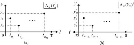
where is the efficacy parameter of feedback control defined as
| (88) |
which is the sum of probabilities of obtaining the time-reversed outcomes by the time-reversed measurements during the time-reversed protocols (see FIG. 3). If holds, Eq. (87) leads to the second generalization of the Jarzynski equality Sagawa-Ueda3 :
| (89) |
If the feedback control in the forward processes is “perfect,” the particle is expected to return to its initial state with unit probability in the backward processes. In such a case, takes the maximum value that equals the number of possible outcomes of . In fact, for the case of the Szilard engine, holds corresponding to and Sagawa-Ueda3 . In contrast, without feedback control, reduces to as
| (90) |
which vindicates the original integral fluctuation theorem. Therefore, the measurements in the backward processes are used to characterized to the efficacy of feedback control in the forward processes.
We stress that and can be measured independently, because is obtained from the forward experiments with feedback and is obtained from the backward experiments without feedback. Therefore, Eqs. (87) and (89) can be directly verified in experiments. In fact, Eq. (89) has been verified in a real experiment by using a feedback-controlled ratchet with a Brownian particle Toyabe3 .
From Eq. (65), we have the second generalization of the second law of thermodynamics
| (91) |
The equality in inequality (91) is achieved if does not fluctuate. We note that, if the distribution of is Gaussian, we have a generalized fluctuation-dissipation theorem
| (92) |
While the first generalization (66) only involves the term of the obtained information, the second generalization (87) involves the term of feedback efficacy. To understand the relationship between the mutual information and the feedback efficacy , we introduce the notation
| (93) |
for any probability variable . We note that, if can be written as with being a real number and being another probability variable, then is the cumulant generation function of . By using this notation, we have
| (94) |
because in Eq. (87), holds as in Eq. (56), and holds as in Eq. (66). Equality (94) implies that is a measure of the correlation between and . This can be more clearly seen by the cumulant expansion of Eq. (94) if the joint distribution of and is Gaussian:
| (95) |
Therefore, characterizes how efficiently we use the obtained information to decrease the entropy production by feedback control: if is large, the more we obtain, the less is.
We can also derive another nonequilibrium equality which also gives us the information about the feedback efficacy. By taking logarithm of the both sides of Eq. (65), we obtain
| (96) |
which is a generalization of Eq. (16). The same result under a different situation has also been obtained in Ref Kawai ; Marin . Equality (96) implies that the renormalized entropy production equals the Kullback-Leibler divergence-like quantity between the forward probability and the backward probability . In fact, without feedback control, the right-hand side of Eq. (96) reduces to the Kullback-Leibler divergence between and and therefore the both sides of Eq. (96) are positive, which is consistent with the second law of thermodynamics. On the contrary, in the presence of feedback control, the right-hand side is no longer the Kullback-Leibler divergence, because is not a normalized probability distribution in terms of . Therefore the both sides of (96) can be negative. Since , the entropy production is bounded from below by the right-hand side of Eq. (96):
| (97) |
Without feedback control, the right-hand side of (97) gives a positive bound, while, with feedback control, the right-hand side can give a negative bound. We note that, for a quantum generalization of the Szilard engine with multi-particles, essentially the same result as Eq. (96) has been obtained SWKim .
We note that special cases of our results in this section were obtained elsewhere. We have derived two types of the generalized Jarzynski equality for the cases with a single measurement in the presence of a single heat bath in Ref. Sagawa-Ueda3 . In Ref. Horowitz , the detailed fluctuation theorem and the Jarzynski equality were obtained for the cases with multi-measurements and feedback in the presence of a single heat bath. In Ref. Suzuki2 , a generalized Jarzynski equality was also obtained for the Kalman filter and the optimal control. The results in this paper include all of the above results, and generalize them to the cases of multi-heat baths and non-Markovian measurements.
VI Examples
We now discuss two examples which illustrate the essential features of our general results. We analytically discuss a generalized Szilard engine with measurement errors in Sec. VI A, and numerically discuss a feedback-controlled ratchet in Sec. VI B.
VI.1 Szilard Engine with Measurement Errors
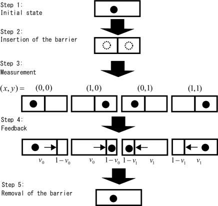
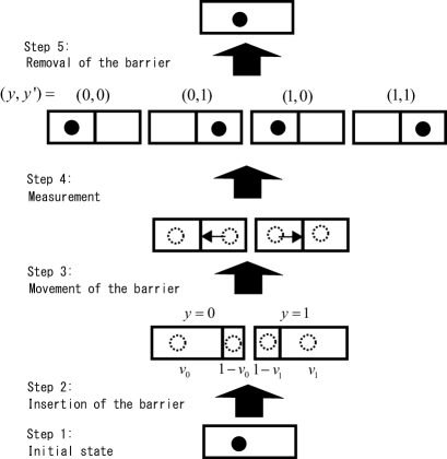
As an example with a classical measurement, we discuss a generalized Szilard engine with measurement errors, which will be shown to achieve the upper bound of inequality (72)or (73) for an arbitrary error rate. The control protocol of the generalized Szilard engine is given by the following steps, which are described FIG. 4.
Step 1: Initial state. A single-particle classical gas is in a box. The initial state of the gas is in thermal equilibrium with a single heat bath at temperature .
Step 2: Insertion of the barrier. We insert a barrier in the middle of the box, and divide it to two boxes with the same volume. Here, we do not know in which box the particle is. For simplicity of notations, we write “left” as “” and “right” as “.” In other words, the position of the particle is given by or . We do not need any work during this process as proved in SWKim .
Step 3: Measurement. We measure the position of the particle. We assume that the measurement is equivalent to the binary symmetric channel with error rate Cover-Thomas ; the measurement outcome takes or , and the measurement error is characterized by conditional probabilities and with . We note that holds for the original Szilard engine without error ().
Step 4: Feedback. We next move the position of the barrier quasi-statically and isothermally. The protocol of moving the barrier depends on measurement outcome . Let () and () be real numbers. We assume that, after we move the barrier, the ratio of the volumes of the boxes is assumed to be for , or for . We note that, in the case of the original Szilard engine, holds. In this process, we extract the work from the engine. The amounts of the work are given by if , if , if , and if . The feedback protocol is characterized by and .
Step 5: Removal of the barrier. We remove the barrier without any work. The engine then returns to the initial state.
From the total process, we extract the average work
| (98) |
We note that holds. We then maximize under a given measurement error by changing and . The maximum value of is achieved when
| (99) |
for which the maximum work is given by
| (100) |
On the other hand, the mutual information of the binary symmetric channel is given by
| (101) |
Therefore, we obtain
| (102) |
which means that the generalized Szilard engine achieves the upper bound of the extractable work (72) or (73) for any amount of the mutual information.
We also check the generalized Jarzynski equalities in this model for arbitrary , , and . We first note that is given by when , when , when , and when . Therefore we obtain
| (103) |
which confirms Eq. (71).
We next consider the second generalization (89) of the Jarzynski equality. Corresponding to two measurement outcomes , we have two backward control protocols as follows (see also FIG. 5).
Step 1. Initial state. The initial state of the backward control is in the thermal equilibrium.
Step 2. Insertion of the barrier. Corresponding to Step 5 of the forward process, we insert the barrier and decide the box into two boxes, because the time-reversal of the barrier removal is the barrier insertion. Corresponding to or in the forward process, we divide the box with the ratio or , respectively.
Step 3. Moving the barrier. We next move the barrier to the middle of the box quasi-statically and isothermally. This is the time-reversal of the feedback control in Step 4 of the forward process.
Step 4. Measurement. We perform the measurement to find in which box the particle is in. Corresponding to the backward protocol with , we obtain the outcomes of backward measurement with probability and with probability . On the other hand, corresponding to the backward protocol with , we obtain the outcomes of backward measurement with probability and with probability .
Step 5. Removal of the barrier. We remove the barrier and the system returns to the initial state. This is the time-reversal of the barrier insertion in Step 2 of the forward process.
From Step 4 of the backward process, we have
| (104) |
On the other hand, we can straightforwardly obtain
| (105) |
which confirms Eq. (89).
VI.2 Feedback-controlled Ratchet
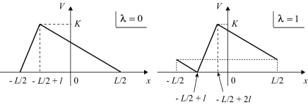
We next discuss a model for Brownian motors Vale ; Prost ; Parrondo2 ; Reimann ; Hanggi1 ; Hanggi2 , in particular a feedback-controlled ratchet Cao1 ; Lopez ; Cao3 . We consider a rotating Brownian particle with a periodic boundary condition. Let be the position or the angle of the particle, and its boundary condition is given by with being a constant. In the following, we restrict the particle’s position to . We assume that the particle obeys the overdamped Langevin equation Eq. (32), and that control parameter takes two values ( or ). Corresponding to them, the ratchet potential takes the following two profiles (FIG. 6):
| (110) | |||||
| (117) |
where is a constant with , and is a positive constant that characterizes the height of the potential.
We start with the initial equilibrium with parameter , and control the system from time to with the following three protocols.
-
1.
Trivial control. We do not change the parameter .
-
2.
Flashing ratchet. At times with being integers and being a constant, we switch parameter from to or from to periodically.
-
3.
Feedback-controlled ratchet. At times , we switch the parameter with the following feedback protocol. We measure the position at without error. We then set from to if and only if the outcome is in . Otherwise, parameter is set to .
For numerical simulations, we set , , , and , with units , , and . We performed the simulations by discretizing Eq. (32) with for samples. We note that, to obtain the initial thermal equilibrium, we waited and checked that the system was fully thermalized in the periodic ratchet with parameter .
The time evolution of the ensemble average is plotted in FIG. 7 (a) for the above three protocols. As expected, nothing happens for the first protocol, while the particle is transported to the right on average for the second and third protocols. In the case of the feedback-controlled ratchet, the particle is transported to the right faster than the case of the flashing ratchet. Figure 7 (b) shows the time evolution of the work that is performed on the particle. The work is induced only in the switching times. We find that, in order to transport the particle, the energy input to the particle with feedback control is smaller than that with the flashing.
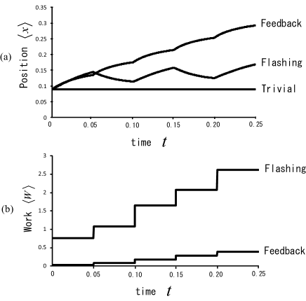
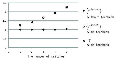
Figure 8 shows the left-hand side of the Jarzynski equality for the flashing and feedback-controlled ratchet, and the efficacy parameter for the feedback-controlled ratchet. We note that always holds. With feedback control, increases from as the number of switchings increases, while, without feedback control, converges to for all switching times in consistent with the original Jarzynski equality. On the other hand, to obtain , we numerically performed the backward experiments. The discretization of the time is , and the number of the samples is for each trajectory of . We note that the number of the trajectories of is given by with times of switchings. Figure 8 shows a good coincidence between and , which confirms the validity of Eq. (89) in the feedback-controlled ratchet.
VII Conclusions
In this paper, we have studied the effects of measurements and feedback control on nonequilibrium thermodynamic systems. In particular, we have generalized nonequilibrium equalities to the systems that are subject to feedback control. Our formulations and results are applicable to a broad class of classical nonequilibrium systems.
In Sec. II, we reviewed stochastic thermodynamics, by focusing on the nonequilibrium equalities. In Sec. III, we formulated measurements on nonequilibrium systems, and defined mutual information by (31) for multi-measurements. In Sec. IV, we formulated feedback control on nonequilibrium systems. We discussed the properties of the joint probability (47), which is well-defined due to causality. We introduced the mutual information by (55), which is not equivalent to in the presence of feedback control. In fact, describes the correlation between the system and the outcomes, which characterizes the effective information obtained by the measurements. We have also shown that the detailed fluctuation theorem (58) holds in the presence of feedback control.
Section V constitutes the main results of this paper. We derived two types of generalizations of the nonequilibrium equalities. In Sec. V A, we derived a generalized detailed fluctuation theorem (65) which involves the mutual information. Based on Eq. (65), we derived the generalizations of the integral fluctuation theorem (66), the Jarzynski equality (71), the second laws (67) (72) (73), the fluctuation-dissipation theorem (70), and the KPB equality (68) that all involve the mutual information. In Sec. V B, we derived the renormalized detailed fluctuation theorem (83), and derived the generalizations of the integral fluctuation theorem (87), the Jarzynski equality (89), the second law (91), the fluctuation-dissipation theorem (92), and the KPB equality (96). We have shown that mutual information , rather than , plays the crucial role to formulate the nonequilibrium equalities under feedback control. These results are the generalizations of the fundamental equalities in nonequilibrium statistical mechanics to feedback-controlled processes, and lead to the generalized second law of thermodynamics with feedback control, which gives the minimal energy cost that is needed for the feedback control.
In Sec. VI, we discussed simple examples to explicitly show that our results in Sec. V can be applied to typical situations. In Sec. VI A, we discussed the Szilard engine with measurement errors that achieves the equality of the generalized second law of thermodynamics (72) or (73). This is an important model to quantitatively illustrate that the mutual information can be converted to the work. We also confirmed the two generalized Jarzynski equalities (71) (89) in the generalized Szilard engine. In Chap. VI B, we considered a feedback-controlled ratchet and confirmed a generalized Jarzynski equality (89).
All of our formulations and results are consistent with the original nonequilibrium equalities and the second law of thermodynamics, and our results serve as the fundamental principle of nonequilibrium thermodynamics of feedback control. We note that, in our results such as Eq. (65), the thermodynamic quantities and the information contents are treated on an equal footing. Therefore, our theory may be regarded as the nonequilibrium version of “information thermodynamics” Sagawa-Ueda1 ; Sagawa-Ueda2 , which serves as the fundamental theory of nonequilibrium information heat engines.
Appendix A Physical Meaning of the Entropy Production
In this appendix, we discuss the physical meanings of the entropy production in the following two typical setups to clarify the typical situations to which our results apply.
Isothermal processes. We assume that there is a single heat bath at temperature , and that the initial distributions of both forward and backward experiments are in the canonical distributions. We stress that we do not assume that the final distributions of both the forward and backward experiments are in the canonical distributions: the final distribution of the forward (backward) experiments does not necessarily equal the initial distribution of the backward (forward) experiments. Let be the Hamiltonian of the system with the time symmetry . The canonical distribution with parameter is given by
| (118) |
where
| (119) |
is the Helmholtz free energy. In this situation, the entropy production reduces to
| (120) |
where
| (121) |
is the work performed on the system from the external parameter, and is the free-energy difference. In this case, Eq. (14) leads to the Jarzynski equality (19), and the second law (15) reduces to inequality (20).
Transition between arbitrary nonequilibrium states: We assume that there are several heat baths, and that we can control the strength of interaction between the system and the baths through . In other words, we can attach or detach the system from the baths by controlling ; for example, we can attach an adiabatic wall to the system. We set an arbitrary initial distribution for the forward experiments. On the other hand, the initial state of the backward experiments is assumed to be taken as , where is the final distribution of the forward experiments. Although this choice of the backward initial state is artificial and is difficult to be experimentally realized except for special cases, this backward initial state is a theoretically useful tool to derive a version of the second law of thermodynamics as follows. In this case, the entropy production is given by
| (122) |
and its ensemble average leads to
| (123) |
where
| (124) |
is the Shannon entropy at time . By introducing notation , the second law (15) leads to
| (125) |
Acknowledgements.
We are grateful to Y. Fujitani, H. Hayakawa, H. Hasegawa, J. M. Horowitz, S. Ito, K. Kawaguchi, T. S. Komatsu, N. Nakagawa, K. Saito, M. Sano, S. Sasa, H. Suzuki, H. Tasaki, and S. Toyabe for valuable discussions. This work was supported by a Grant-in Aid for Scientific Research on Innovative Areas “Topological Quantum Phenomena” (KAKENHI 22103005) from the Ministry of Education, Culture, Sports, Science and Technology (MEXT) of Japan, and by a Global COE program “Physical Science Frontier” of MEXT, Japan. TS acknowledges JSPS Research Fellowships for Young Scientists (Grant No. 208038) and the Grant-in-Aid for Research Activity Start-up (Grant No. 11025807).References
- (1) J. C. Doyle, B. A. Francis, and A. R. Tannenbaum, “Feedback Control Theory,” (Macmillan, New York, 1992).
- (2) K. J. Åstrom and R. M. Murray, “Feedback Systems: An Introduction for Scientists and Engineers,” ( Princeton University Press, 2008).
- (3) K. Sekimoto, Prog. Theor, Phys. Suppl. 130, 17 (1998).
- (4) C. Bustamante, J. Liphardt, and F. Ritort, Physics Today, 58 43 (2005).
- (5) U. Seifert, Euro. Phys. J. B 64 423 (2008).
- (6) D. J. Evans, E. G. D. Cohen, and G. P. Morriss, Phys. Rev. Lett. 71, 2401 (1993).
- (7) G. Gallavotti, and E. G. D. Cohen, Phys. Rev. Lett. 74, 2694 (1995).
- (8) C. Jarzynski, Phys. Rev. Lett. 78, 2690 (1997).
- (9) J. Kurchan, J. Phys. A. Math. Gen. 31, 3719 (1998).
- (10) G. E. Crooks, J. Stat. Phys. 90, 1481 (1998).
- (11) G. E. Crooks, Phys. Rev. E 60, 2721 (1999).
- (12) J. L. Lebowitz and H. Spohn, J. Stat. Phys. 95, 333 (1999).
- (13) C. Maes, J. Stat. Phys. 95, 367 (1999).
- (14) C. Maes, F. Redig, and A. Van Moffaert, J. Math. Phys. 41 1528 (2000).
- (15) C. Jarzynski, J. Stat. Phys. 98, 77 (2000).
- (16) J. Kurchan, arXiv:cond-mat/0007360 (2000).
- (17) H. Tasaki, arXiv:cond-mat/0009244 (2000).
- (18) T. Hatano and S.-I. Sasa, Phys. Rev. Lett. 86, 3463 (2001).
- (19) D. J. Evans and D. J. Searles, Adv. Phys. 51, 1529 (2002).
- (20) R. van Zon and E. G. D. Cohen, Phys. Rev. Lett. 91, 110601 (2003).
- (21) C. Jarzynski, J. Stat. Mech: Theor. Exp. P09005 (2004).
- (22) C. Jarzynski and D. K. Wójcik, Phys. Rev. Lett. 92, 230602 (2004).
- (23) T. Harada and S.-I. Sasa, Phys. Rev. Lett. 95, 130602 (2005).
- (24) U. Seifert, Phys. Rev. Lett. 95, 040602 (2005).
- (25) M. Esposito and S. Mukamel, Phys. Rev. E 73, 046129 (2006).
- (26) D. Andrieux and P. Gaspard, J. Stat. Mech. P02006 (2007).
- (27) K. Saito and A. Dhar, Phys. Rev. Lett. 99, 180601 (2007).
- (28) T. Ohkuma and T. Ohta J. Stat. Mech. P10010 (2007).
- (29) R. Kawai, J. M. R. Parrondo, and C. Van den Broeck, Phys. Rev. Lett. 98, 080602 (2007).
- (30) A. Gomez-Marin, J. M. R. Parrondo, and C. Van den Broeck, Phys. Rev. E 78, 011107 (2008).
- (31) T. S. Komatsu and N. Nakagawa, Phys. Rev. Lett. 100, 030601 (2008).
- (32) T. S. Komatsu, N. Nakagawa, S. I. Sasa, and H. Tasaki, Phys. Rev. Lett. 100, 230602 (2008).
- (33) Y. Utsumi and K. Saito, Phys. Rev. B 79, 235311 (2009).
- (34) M. Campisi, P. Talkner, and P. Hänggi, Phys. Rev. Lett. 102, 210401 (2009).
- (35) J. Ren, P. Hänggi, and B. Li, Phys. Rev. Lett. 104, 170601 (2010).
- (36) H. Hasegawa, J. Ishikawa, K. Takara, and D.J. Driebe, Phys. Lett. A 374, 1001 (2010).
- (37) M. Esposito and C. Van den Broeck, Phys. Rev. Lett. 104, 090601 (2010).
- (38) M. Campisi, P. Talkner and P. Hänggi, Phys. Rev. Lett. 105, 140601 (2010)
- (39) S. Vaikuntanathan and C. Jarzynski, Euro. Phys. Lett. 87, 60005 (2010).
- (40) G. M. Wang et al., Phys. Rev. Lett. 89, 050601 (2002).
- (41) J. Liphardt et al., Science 296, 1832 (2002).
- (42) E. H. Trepagnier et al., Proc. Natl. Acad. Sci. U.S.A. 101, 15038 (2004).
- (43) D. M. Carberry et al., Phys. Rev. Lett. 92, 140601 (2004).
- (44) D. Collin et al., Nature 437, 231 (2005).
- (45) F. Douarche et al., Phys. Rev. Lett. 97, 140603 (2006).
- (46) D. Andrieux et al., Phys. Rev. Lett. 98, 150601 (2007).
- (47) S. Toyabe et al., Phys. Rev. E 75, 011122 (2007).
- (48) S. Toyabe et al., Phys. Rev. Lett. 104, 198103 (2010).
- (49) K. Hayashi et al., Phys. Rev. Lett. 104, 218103 (2010).
- (50) S. Nakamura et al., Phys. Rev. Lett. 104, 080602 (2010).
- (51) V. Serreli et al., Nature 445, 523 (2007).
- (52) S. Rahav, J. Horowitz, and C. Jarzynski, Phys. Rev. Lett. 101, 140602 (2008).
- (53) E. R. Kay, D. A. Leigh, and F. Zerbetto, Angew. Chem. 46, 72 (2007).
- (54) H. Gu et al., Nature 465 , 202 (2010).
- (55) M. Schliwa and G. Woehlke, Nature 422, 759 (2003).
- (56) F. J. Cao, L. Dinis, J. M. R. Parrondo, Phys. Rev. Lett. 93, 040603 (2004).
- (57) K. H. Kim and H. Qian, Phys. Rev. E 75, 022102 (2007).
- (58) B. J. Lopez et al., Phys. Rev. Lett. 101, 220601 (2008).
- (59) F. J. Cao and M. Feito, Phys. Rev. E 79, 041118 (2009).
- (60) M. Feito, J. P. Baltanas, and F. J. Cao, Phys. Rev. E 80, 031128 (2009).
- (61) M. Bonaldi et al., Phys. Rev. Lett. 103, 010601 (2009).
- (62) H. Suzuki and Y. Fujitani, J. Phys. Soc. Jpn. 78, 074007 (2009).
- (63) T. Sagawa and M. Ueda, Phys. Rev. Lett. 104, 090602 (2010).
- (64) Y. Fujitani and H. Suzuki, J. Phys. Soc. Jpn. 79, 104003 (2010).
- (65) T. Brandes, Phys. Rev. Lett. 105, 060602 (2010).
- (66) M. Ponmurugan, Phys. Rev. E 82, 031129 (2010).
- (67) J. M. Horowitz and S. Vaikuntanathan, Phys. Rev. E 82, 061120 (2010).
- (68) Y. Morikuni and H. Tasaki, J. Stat. Phys. 13, 1 (2011)
- (69) D. Abreu and U. Seifert, Euro. Phys. Lett. 94, 10001 (2011).
- (70) J. M. Horowitz and J. M. R. Parrondo, Euro. Phys. Lett. 95, 10005 (2011).
- (71) M. Esposito and C. Van den Broeck, Euro. Phys. Lett. 95, 40004 (2011).
- (72) S. Vaikuntanathan and C. Jarzynski, Phys. Rev. E 83, 061120 (2011).
- (73) T. Sagawa, J. Phys.: Conf. Ser. 297, 012015 (2011).
- (74) S. Lahiri, S. Rana, and A. M. Jayannavar, arXiv:1109.6508 (2011).
- (75) D. V. Averin, M. Mottonen, and J. P. Pekola, arXiv:1108.5435 (2011).
- (76) J. M. Horowitz and J. M. R. Parrondo, arXiv:1110.6808 (2011).
- (77) S. Toyabe, T. Sagawa, M. Ueda, E. Muneyuki, and M. Sano, Nature Physics 6, 988 (2010).
- (78) J. C. Maxwell, “Theory of Heat,” (Appleton, London, 1871).
- (79) “Maxwell’s demon 2: Entropy, Classical and Quantum Information, Computing”, H. S. Leff and A. F. Rex (eds.), (Princeton University Press, New Jersey, 2003).
- (80) L. Szilard, Z. Phys. 53, 840 (1929).
- (81) L. Brillouin, J. Appl. Phys. 22, 334 (1951).
- (82) C. H. Bennett, Int. J. Theor. Phys. 21, 905 (1982).
- (83) R. Landauer, IBM J. Res. Dev. 5, 183 (1961).
- (84) S. Lloyd, Phys. Rev. A 39, 5378 (1989).
- (85) S. Lloyd and W. H. Zurek, J. Stat. Phys. 62, 819 (1991).
- (86) S. Lloyd, Phys. Rev. A 56, 3374 (1997).
- (87) H. Touchette and S. Lloyd, Phys. Rev. Lett. 84, 1156 (2000).
- (88) W. H. Zurek, quant-ph/0301076 (2003).
- (89) M. O. Scully et al., Science 299, 862 (2003).
- (90) T. D. Kieu, Phys. Rev. Lett. 93, 140403 (2004).
- (91) A. E. Allahverdyan et al., J. Mod. Optics, 51, 2703 (2004).
- (92) H. T. Quan et al., Phys. Rev. Lett. 97, 180402 (2006).
- (93) M. A. Nielsen, C. M. Caves, B. Schumacher, and H. Barnum, Proc. R. Soc. London A, 454, 277 (1998).
- (94) T. Sagawa and M. Ueda, Phys. Rev. Lett. 100, 080403 (2008).
- (95) K. Jacobs, Phys. Rev. A 80, 012322 (2009).
- (96) T. Sagawa and M. Ueda, Phys. Rev. Lett. 102, 250602 (2009); Phys. Rev. Lett. 106, 189901(E) (2011).
- (97) K. Maruyama, F. Nori, and V. Vedral, Rev. Mod. Phys. 81, 1 (2009).
- (98) S. W. Kim, T. Sagawa, S. De Liberato, and M. Ueda, Phys. Rev. Lett. 106, 070401 (2011).
- (99) C. Shannon, Bell System Technical Journal 27, 379-423 and 623-656 (1948).
- (100) T. M. Cover and J. A. Thomas, “Elements of Information Theory” (John Wiley and Sons, New York, 1991).
- (101) G. Welch and G. Bishop, “An introduction to the Kalman filter”, Technical Report TR 95-041, University of North Carolina, Department of Computer Science (1995).
- (102) D. P. Bertsekas, “Dynamic Programming and Optimal Control”, (Athena Scientific 2005).
- (103) R. D. Vale and F. Oosawa, Adv. Biophys. 26, 97 (1990).
- (104) F. Julicher, A. Ajdari, and J. Prost, Rev. Mod. Phys. 69, 1269 (1997).
- (105) J. M. R. Parrondo, B. J. De Cisneros, Appl. Phys. A 75,179 (2002).
- (106) P. Reimann. Phys. Rept. 361, 57 (2002).
- (107) P. Hänggi, F. Marchesoni, and F. Nori, Ann. Phys. 14, 51 (2005).
- (108) P. Hänggi and F. Marchesoni, Rev. Mod. Phys. 81, 387 (2009).