Rigid components in fixed-lattice and cone frameworks

Abstract

We study the fundamental algorithmic rigidity problems for generic frameworks periodic with respect to a fixed lattice or a finite-order rotation in the plane. For fixed-lattice frameworks we give an $O(n^{2})$ algorithm for deciding generic rigidity and an $O(n^{3})$ algorithm for computing rigid components. If the order of rotation is part of the input, we give an $O(n^{4})$ algorithm for deciding rigidity; in the case where the rotation’s order is $3$, a more specialized algorithm solves all the fundamental algorithmic rigidity problems in $O(n^{2})$ time.

1 Introduction

The geometric setting for this paper involves two variations on the well-studied planar bar-joint rigidity model: fixed-lattice periodic frameworks and cone frameworks. A fixed-lattice periodic framework is an infinite structure, periodic with respect to a lattice, where the allowed continuous motions preserve, the lengths and connectivity of the bars, as well as the periodicity with respect to a fixed lattice. See Figure 1(a) for an example. A cone framework is also made of fixed-length bars connected by universal joints, but it is finite and symmetric with respect to a finite order rotation; the allowed continuous motions preserve the bars’ lengths and connectivity and symmetry with respect to a fixed rotation center. Cone frameworks get their name from the fact that the quotient of the plane by a finite order rotation is a flat cone with opening angle $2\pi/k$ and the quotient framework, embedded in the cone with geodesic “bars”, captures all the geometric information [12]. Figure 2(a) shows an example.

A fixed-lattice framework is rigid if the only allowed motions are translations and flexible otherwise. A cone-framework is rigid if the only allowed motions are rotations around the center and flexible otherwise. The alternate formulation for cone frameworks says that rigidity means the only allowed motions are isometries of the cone, which is just rotation around the cone point. A framework is minimally rigid if it is rigid, but ceases to be so if any of the bars are removed.

Generic rigidity

The combinatorial model for the fixed-lattice and cone frameworks introduced above is given by a colored graph $(G,\bm{\gamma})$: $G=(V,E)$ is a finite directed graph and $\bm{\gamma}=(\gamma_{ij})_{ij\in E}$ is an assignment of a group element $\gamma_{ij}\in\Gamma$ (the “color”) to each edge $ij$ for a group $\Gamma$. For fixed-lattice frameworks, the group $\Gamma$ is $\mathbb{Z}^{2}$, representing translations; for cone frameworks it is $\mathbb{Z}/k\mathbb{Z}$ with $k\geq 2$ a natural number. See Figure 1(b) and Figure 2(b).

The colors can be seen as efficiently encoding a map $\rho$ from the oriented cycle space of $G$ into $\Gamma$; $\rho$ is defined, in detail, in Section 2. If the image of $\rho$ restricted to a subgraph $G^{\prime}$ contains only the identity element, we define the $\Gamma$-image of $\rho$ to be trivial otherwise it is non-trivial.

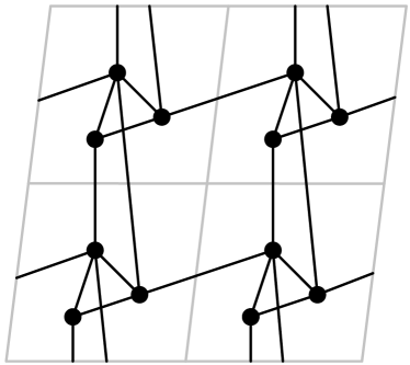
Figure 1: Periodic frameworks and colored graphs: (a) part of a periodic framework, with the representation of the integer lattice $\mathbb{Z}^{2}$ shown in gray and the bars shown in black; (b) one possibility for the the associated colored graph with $\mathbb{Z}^{2}$ colors on the edges. (Graphics from [11].)

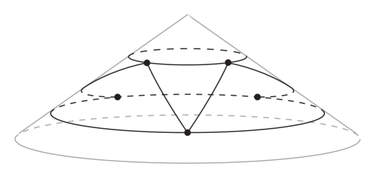
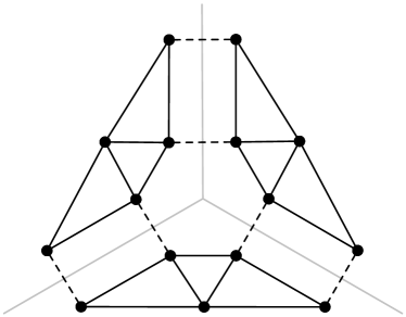
Figure 2: Cone-Laman graphs: (a) a realization of the framework on a cone with opening angle $2\pi/3$ (graphic from Chris Thompson); (b) a $\mathbb{Z}/3\mathbb{Z}$-colored graph (edges without colors have color $0$); (c) the developed graph with $\mathbb{Z}/3\mathbb{Z}$-symmetry (dashed edges are lifts of dashed edges in (b)).

The generic rigidity theory of planar frameworks with, more generally, crystallographic symmetry has seen a lot of progress recently [3, 14, 11, 12]. Elissa Ross [14] announced the following theorem:

Theorem 1.1 ([14, 11]).

A generic fixed-lattice periodic framework with associated colored graph $(G,\bm{\gamma})$ is minimally rigid if and only if: (1) $G$ has $n$ vertices and $2n-2$ edges; (2) all non-empty subgraphs $G^{\prime}$ of $G$ with $m^{\prime}$ edges and $n^{\prime}$ vertices and trivial $\mathbb{Z}^{2}$-image satisfy $m^{\prime}\leq 2n^{\prime}-3$; (3) all non-empty subgraphs $G^{\prime}$ with non-trivial $\mathbb{Z}^{2}$-image satisfy $m^{\prime}\leq 2n^{\prime}-2$.

The colored graphs appearing in the statement of Theorem 1.1 are defined to be Ross graphs; if only conditions (2) and (3) are met, $(G,\bm{\gamma})$ is Ross-sparse. Ross graphs generalize the well-known Laman graphs which are uncolored, have $m=2n-3$ edges, and satisfy (2). By Theorem 1.1 the maximal rigid sub-frameworks of a generic fixed-lattice framework on a Ross-sparse colored graph $(G,\bm{\gamma})$ correspond to maximal subgraphs of $G$ with $m^{\prime}=2n^{\prime}-2$; we define these to be the rigid components of $(G,\bm{\gamma})$. In the sequel, we will also refer to graphs with the Ross property for $\Gamma=\mathbb{Z}/k\mathbb{Z}$ as simply “Ross graphs”.

Malestein and Theran [12] proved a similar statement for cone frameworks:

Theorem 1.2 ([12]).

A generic cone framework with associated colored graph $(G,\bm{\gamma})$ is minimally rigid if and only if: (1) $G$ has $n$ vertices and $2n-1$ edges; (2) all non-empty subgraphs $G^{\prime}$ of $G$ with $m^{\prime}$ edges and $n^{\prime}$ vertices and trivial $\mathbb{Z}/k\mathbb{Z}$-image satisfy $m^{\prime}\leq 2n^{\prime}-3$; (3) all non-empty subgraphs $G^{\prime}$ with non-trivial $\mathbb{Z}/k\mathbb{Z}$-image satisfy $m^{\prime}\leq 2n^{\prime}-1$.

The graphs appearing in the statement of Theorem 1.2 are called cone-Laman graphs. We define cone-Laman-sparse colored graphs and their rigid components similarly to the analogous definitions for Ross-sparse graphs, with $2n^{\prime}-1$ replacing $2n^{\prime}-2$.

Ross and cone-Laman graphs are examples of the “$\Gamma$-graded-sparse” colored graphs introduced in [11, 12]. They are all matroidal families [11, 12], which guarantees that greedy algorithms work correctly on them.

Main results

In this paper we begin the investigation of the algorithmic theory of crystallographic rigidity by addressing the fixed-lattice and cone frameworks. Given a colored graph $(G,\bm{\gamma})$, we are interested in the rigidity properties of an associated generic framework. Lee and Streinu [8] define three fundamental algorithmic rigidity questions: Decision Is the input rigid?; Extraction Find a maximum subgraph of the input corresponding to independent length constraints; Components Find the maximal rigid sub-frameworks of a flexible input.

We give algorithms for these problems with running times shown in the following table

	Decision	Extraction	Components
Fixed-lattice	$O(n^{2})$	$O(n^{3})$	$O(n^{3})$
Cone $k\neq 3$	$O(n^{4})$	$O(n^{5})$	$O(n^{5})$
Cone $k=3$	$O(n^{2})$	$O(n^{2})$	$O(n^{2})$

Novelty

Previously, the only known efficient combinatorial algorithms for any of these problems were pointed out in [11, 12]: the Edmonds Matroid Union algorithm yields an algorithm with running times $O(n^{4})$ for Decision and $O(n^{5})$ Extraction. A folklore randomized algorithm based on Gaussian elimination gives an $O(n^{3}\operatorname{polylog}(n))$ algorithm for Decision and Extraction of most rigidity problems, but this doesn’t easily generalize to Components.

The $O(n^{2})$ running time for Decision for fixed-lattice frameworks equals that from the pebble game [8, 7, 2] for the corresponding problem in finite frameworks. Although there are faster Decision algorithms [4] for finite frameworks, the pebble game is the standard tool in the field due to its elegance and ease of implementation. Our algorithms for cone frameworks with order $3$ rotation are a reduction to the pebble games of [8, 7, 2].

The $O(n^{3})$ running time for Extraction and Components in fixed-lattice frameworks is worse by a factor of $O(n)$ than the pebble games for finite frameworks. However, it is equal to the $O(n^{3})$ running time from [8] for the “redundant rigidity” problem. Computing fundamental Laman circuits (definition in Section 2) plays an important role (though for different reasons) in both of these algorithms.

Roadmap and key ideas

Our main contribution is a pebble game algorithm for Ross graphs, from which we can deduce the corresponding results for general cone-Laman graphs. Intuitively, the algorithmic rigidity problems should be harder for Ross graphs than for Laman graphs, since the number of edges allowed in a subgraph depends on whether the $\mathbb{Z}^{2}$-image of the subgraph is trivial or not. To derive an efficient algorithm we use three key ideas (detailed definitions are given in Section 2):

• The Lee-Streinu-Theran [10] approach of playing several copies of the pebble game for $(k,\ell)$-graphs [8] with different parameters to handle different sparsity counts for different types of subgraphs.

• A new structural characterization of the edge-wise minimal colored graphs which violate the Ross counts (Section 3).

• A linear time algorithm for computing the $\Gamma$ image of a given subgraph (Section 4).

Our algorithms for general cone-Laman graphs then use the Ross graph Decision algorithm as a subroutine. When the order of the rotation is $3$, we can reduce the cone-Laman rigidity questions to Laman graph rigidity questions directly, resulting in better running times.

Motivation

Periodic frameworks, in which the lattice can flex, arise in the study of zeolites, a class of microporous crystals with a wide variety of industrial applications, notably in petroleum refining. Because zeolites exhibit flexibility [15], computing the degrees of freedom in potential [13, 17] zeolite structures is a well-motivated algorithmic problem.

Other related work

The general subject of periodic and crystallographic rigidity has seen a lot of progress recently, see [6] for a list of announcements. Bernd Schulze [16] has studied Laman graphs with a free $\mathbb{Z}/3\mathbb{Z}$ action in a different context.

2 Preliminaries

In this section, we introduce the required background in colored graphs, hereditary sparsity, and introduce a data structure for least common ancestor queries in trees that is an essential tool for us.

Colored graphs and the map $\rho$

A pair $(G,\bm{\gamma})$ is defined to be a colored graph with $\Gamma$ a group, $G=(V,E)$ a finite, directed graph on $n$ vertices and $m$ edges, and $\bm{\gamma}=(\gamma_{ij})_{ij\in E}$ is an assignment of a group element $\gamma\in\Gamma$ to each edge.

Let $(G,\bm{\gamma})$ be a colored graph, and let $C$ be a cycle in $G$ with a fixed traversal order. We define $\rho(C)$ to be

$$\rho(C)=\sum_{\begin{subarray}{c}ij\in C\\ \text{$ij$ traversed}\\ \text{ forwards}\end{subarray}}\gamma_{ij}-\sum_{\begin{subarray}{c}ij\in C\\ \text{$ij$ traversed}\\ \text{backwards}\end{subarray}}\gamma_{ij}$$

Since $\Gamma$ is always abelian in this paper, we need not be concerned with the particular order of summation; our notation doesn’t capture the specific traversal of $C$, but this is not important here since we are interested in whether $\rho(C)$ is trivial or not, which doesn’t depend on sign. For a subgraph $G^{\prime}$ of $G$, we define $\rho(G^{\prime})$ to be trivial if its image on cycles spanned by $G^{\prime}$ contains only the identity and non-trivial otherwise. We need the following fact about $\rho$.

Lemma 2.1 ([11, Lemma 2.2]).

Let $(G,\bm{\gamma})$ be a colored graph. Then $\rho(G)$ is trivial if and only if, for any spanning forest $T$ of $G$, $\rho$ is trivial on every fundamental cycle induced by $T$.

$(k,\ell)$-sparsity and pebble games

The hereditary sparsity counts defining Ross and cone-Laman graphs generalize to $(k,\ell)$-sparse graphs which satisfy “$m^{\prime}\leq kn^{\prime}-\ell$” for all subgraphs; if in addition the total number of edges is $m=kn-\ell$, the graph is a $(k,\ell)$-graph. We also need the notion of a $(k,\ell)$-circuit, which is an edge-minimal graph that is not $(k,\ell)$-sparse; these are always $(k,\ell-1)$-graphs [8]. If $G$ is any graph, a $(k,\ell)$-basis of $G$ is a maximal subgraph that is $(k,\ell)$-sparse; if $G^{\prime}$ is a $(k,\ell)$-basis of $G$ and $ij\in E(G)-E(G^{\prime})$, the fundamental $(k,\ell)$-circuit of $ij$ with respect to $G^{\prime}$ is the unique (see [8]) $(k,\ell)$-circuit in $G^{\prime}+{ij}$. See [8] for a detailed development of this theory. As is standard in the field, we use “$(2,3)$-” and “Laman” interchangeably.

Although $(k,\ell)$-sparsity is defined by exponentially many inequalities on subgraphs, it can be checked in quadratic time using the pebble game [8], an elegant incremental approach that builds a $(k,\ell)$-sparse graph $G$ one edge at a time. Here, we will use the pebble game as a “black box” to: (1) Check if an edge $ij$ is in the span of any $(k,\ell)$-component of $G$ in $O(1)$ time [8, 9]; (2) Assuming that $G$ plus a new edge $ij$ is $(k,\ell)$-sparse, add the edge $ij$ to $G$ and update the components in amortized $O(n^{2})$ time [8]; (3) Compute the fundamental circuit with respect to a given $(k,\ell)$-sparse graph $G$ in $O(n)$ time [8].

Least common ancestors in trees

Let $T$ be a rooted tree with root $r$ and $i$ and $j$ be any vertices in $T$. The least common ancestor (shortly, LCA) of $i$ and $j$ is defined to be the vertex where the (unique, since $T$ is a tree) paths from $i$ to $r$ and $j$ to $r$ first converge. If either $i$ or $j$ is $r$, then this is just $r$. A fundamental result of Harel and Tarjan [5] is that LCA queries can be answered in $O(1)$ time after $O(n)$ preprocessing.

3 Combinatorial lemmas

In this section we prove structural properties of Ross and cone-Laman graphs that are required by our algorithms.

Ross graphs

Let $(G,\bm{\gamma})$ be a colored graph and suppose that $G$ is a $(2,2)$-graph. We can verify that $(G,\bm{\gamma})$ is Ross by checking the $\mathbb{Z}^{2}$-images of a relatively small set of subgraphs.

Lemma 3.1.

Let $(G,\bm{\gamma})$ be a colored graph and suppose that $G$ is a $(2,2)$-graph. Then $(G,\bm{\gamma})$ is a Ross graph if and only if for any Laman basis $L$ of $G$, the fundamental Laman circuit with respect to $L$ of every edge $ij\in E-E(L)$ has non-trivial $\mathbb{Z}^{2}$-image.

Figure 3 shows two examples. The important point is that we can pick any Laman basis $L$ of $G$. The proof is deferred to Appendix A. The main idea is that $G$ being a $(2,2)$-graph forces all Laman circuits to be edge-disjoint, from which we can deduce all of them are fundamental Laman circuits of every Laman basis.

Figure 3: Examples of Ross and non-Ross graphs (edges without colors have color $(0,0)$): (a) a Ross graph; the underlying graph is itself a Laman circuit; (b) the underlying graph is a $(2,2)$-graph, but the uncolored $K_{4}$ subgraph has trivial image, so this is not a Ross graph. Note that $K_{4}$ is a Laman circuit, illustrating Lemma 3.1

Cone-Laman graphs

Because cone-Laman graphs have an underlying $(2,1)$-graph, the statement of Lemma 3.1, with $(2,1)$- replacing $(2,2)$- does not hold for cone-Laman graphs. Figure 4 shows a counterexample. The analogous statement, proven in Appendix B is:

Lemma 3.2.

Let $(G,\bm{\gamma})$ be a colored graph. Then $(G,\bm{\gamma})$ is a cone-Laman graph if and only if: (1) $G$ is a $(2,1)$-graph; (2) for any $(2,2)$-basis $R$ of $G$, the fundamental $(2,2)$-circuit $G^{\prime}$ with respect to $R$ of $ij\in E(G)-E(R)$ becomes a Ross graph after removing any edge from $G^{\prime}$; (3) for any Laman-basis $L$ of $G$, the fundamental Laman-circuits with respect to $L$ have non-trivial $\Gamma$-image.

Order three rotations

In the special case where the group $\Gamma=\mathbb{Z}/3\mathbb{Z}$, which corresponds to a cone with opening angle $2\pi/3$, we can give a simpler characterization of cone-Laman graphs in terms of their development. The development $\tilde{G}$ is defined by the following construction: $\tilde{G}$ has three copies of each vertex $i$: $i_{0}$, $i_{1}$ and $i_{2}$; a directed edge $ij$ with color $\gamma$ then generates three undirected edges $i_{k}j_{k+\gamma}$ (addition is modulo 3). See Figure 2(c)) for an example. The development has a free $\mathbb{Z}/3\mathbb{Z}$-action; a subgraph of $\tilde{G}$ is defined to be symmetric if it is fixed by this action. In Appendix C we prove.

Lemma 3.3.

Let $(G,\bm{\gamma})$ be a colored graph with $\Gamma=\mathbb{Z}/3\mathbb{Z}$. Then $(G,\bm{\gamma})$ is a cone-Laman graph if and only if its development $\tilde{G}$ is a Laman graph. Moreover, the rigid components of $(G,\bm{\gamma})$ correspond to the symmetric rigid components of $\tilde{G}$.

4 Computing the $\Gamma$-image of $\rho$

We now focus on the problem of deciding whether the $\Gamma$-image of the map $\rho$, defined in Section 2, is trivial on a colored graph $(G,\bm{\gamma})$. The case in which $G$ is not connected follows easily by considering connected components one at a time, so we assume from now on that $G$ is connected. Let $(G,\bm{\gamma})$ be a colored graph and $T$ be a spanning tree of $G$ with root $r$. For a vertex $i$, there is a unique path $P_{i}$ in $T$ from $r$ to $i$. We define $\sigma_{ri}$ to be

$$\sigma_{ri}=\sum_{\begin{subarray}{c}jk\in P_{i}\\ \text{$jk$ traversed forwards}\end{subarray}}\gamma_{jk}-\sum_{\begin{subarray}{c}jk\in P_{i}\\ \text{$jk$ traversed backwards}\end{subarray}}\gamma_{jk}$$

The notation $\sigma_{ri}$ extends in a natural way: for a a vertex $j$ on $P_{i}$, we define $\sigma_{ij}$ to be $\sigma_{ri}-\sigma_{rj}$; if $\sigma_{ji}$ is defined, we define $\sigma_{ij}=-\sigma_{ji}$. The key observation is the following lemma.

Lemma 4.1.

Let $(G,\bm{\gamma})$ be a connected colored graph, let $T$ be a rooted spanning tree of $G$, let $ij$ be an edge of $G$ not in $T$, and let $a$ be the least common ancestor of $i$ and $j$. Then, if $C$ is the fundamental cycle of $ij$ with respect to $T$, $\rho(C)=\sigma_{ai}+\gamma_{ij}-\sigma_{ja}$.

Proof 4.2.

Traversing the fundamental cycle of $ij$ so that $ij$ is crossed from $i$ to $j$ means: going from $i$ to $j$, from $j$ to the LCA $a$ of $i$ and $j$ towards the root, and then from $a$ to $i$ away from the root.

We now show how to compute whether the $\Gamma$-image of a colored graph is trivial in linear time. The idea used here is closely related to a folklore $O(n^{2})$ algorithm for all-pairs-shortest paths in trees.

Lemma 4.3.

Let $(G,\bm{\gamma})$ be a connected colored graph with $n$ vertices and $m$ edges. There is an $O(n+m)$ time algorithm to decide whether the $\Gamma$-image of $\rho(G)$ is trivial.

The rest of this section gives the proof of Lemma 4.3. We first present the algorithm.
Input: A colored graph $(G,\bm{\gamma})$
Question: Is $\rho(G)$ trivial?
Method:

• Pick a spanning tree $T$ of $G$ and root it.

• Compute $\sigma_{ri}$ for each vertex $i$ of $G$.

• For each edge $ij$ not in $T$, compute the image of its fundamental cycle in $T$.

• Say ‘yes’ if any of these images are not the identity and ‘no’ otherwise.

Correctness

This is an immediate consequence of Lemma 2.1, since the algorithm checks all the fundamental cycles with respect to a spanning tree.

Running time

Finding the spanning tree with BFS is $O(m)$ time, and once the tree is computed, the $\sigma_{ri}$ can be computed with a single pass over it in $O(n)$ time. Lemma 4.1 says that the image of any fundamental cycle with respect to $T$ can be computed in $O(1)$ time once the LCA of the endpoints of the non-tree edge is known. Using the Harel-Tarjan data structure, the total cost of LCA queries is $O(n+m)$, and the running time follows.

The pebble game for Ross graphs

We have all the pieces in place to describe our algorithm for the rigidity problems in Ross graphs.

Algorithm: Rigid components in Ross graphs

Input: A colored graph $(G,\bm{\gamma})$ with $n$ vertices and $m$ edges.
Output: The rigid components of $(G,\bm{\gamma})$.
Method: We will play the pebble game for $(2,3)$-sparse graphs and the pebble game for $(2,2)$-sparse graphs in parallel. To start, we initialize each of these separately, including data structures for maintaining the $(2,2)$- and $(2,3)$-components.

Then, for each colored edge $ij\in E$:

• If $ij$ is in the span of a $(2,2)$-component in the $(2,2)$-sparse graph we are maintaining, we discard $ij$ and proceed to the next edge.

• If $ij$ is not in the span of any $(2,3)$-component, we add $ij$ to both the $(2,2)$-sparse and $(2,3)$-sparse graphs we are building, and update the components of each.

• Otherwise, we use the $(2,3)$-pebble game to identify the smallest $(2,3)$-block $G^{\prime}$ spanning $ij$. We add $ij$ to this subgraph $G^{\prime}$ and compute its $\mathbb{Z}^{2}$-image. If this is trivial, we discard $ij$ and proceed to the next edge.

• If the image of $G^{\prime}$ was non-trivial, add $ij$ to the $(2,2)$-sparse graph we are maintaining and update its rigid components.

The output is the (2,2)-components in the $(2,2)$-sparse graph we built.

Correctness

By definition, the rigid components of a Ross graph are its $(2,2)$-components. Step (A) ensures that we maintain a $(2,2)$-sparse graph; steps (B) and (C), by Lemma 3.1 imply that when new $(2,2)$-blocks are formed all of them have non-trivial $\mathbb{Z}^{2}$-image, which is what is required for Ross-sparsity. Step (D) ensures that the rigid components are updated at every step. The matroidal property implies that a greedy algorithm is correct.

Running time

By [8, 9], steps (A), (B), and (D) require $O(n^{2})$ time over the entire run of the algorithm (the analysis of the time taken to update components is amortized). Step (C), by [8] and Lemma 4.1 requires $O(n)$ time. Since $\Omega(m)$ iterations may enter step (C), this becomes the bottleneck, resulting in an $O(nm)$ running time, which is $O(n^{3})$.

Modifications for other rigidity problems

We have presented and analyzed an algorithm for computing the rigid components in Ross graphs. Minor modifications give solutions to the Decision and Extraction problems. For Extraction, we just return the $(2,2)$-sparse graph we built; the running time remains $O(n^{3})$. For Decision, we simply stop and say ‘no’ if any edge is ever discarded. Since we process at most $O(n)$ edges, the running time becomes $O(n^{2})$.

5 Pebble games for cone-Laman graphs

We now describe our algorithms for cone-Laman graphs.

Order-three rotations

We start with the special case when the group $\Gamma=\mathbb{Z}/3\mathbb{Z}$. In this case, the following algorithm’s correctness is immediate from Lemma 3.3. The running time follows from [8, 9, 2] and the fact that the development can be computed in linear time.

Input: A colored graph $(G,\bm{\gamma})$ with $n$ vertices and $m$ edges.
Output: The rigid components of $(G,\bm{\gamma})$.
Method:

• Compute the development $\tilde{G}$ of $(G,\bm{\gamma})$.

• Use the $(2,3)$-pebble game to compute the rigid components of $\tilde{G}$.

• Return the subgraphs of $G$ corresponding to the symmetric rigid components in $\tilde{G}$.

General cone-Laman graphs

For colored graphs with $\Gamma=\mathbb{Z}/k\mathbb{Z}$, we don’t have an analogue of Lemma 3.3, and the development may not be polynomial size. However, we can modify our pebble game for Ross graphs to compute the rigid components. Here is the algorithm: Input: A colored graph $(G,\bm{\gamma})$ with $n$ vertices and $m$ edges, and an integer $k$.
Output: The rigid components of $(G,\bm{\gamma})$.
Method: We initialize a $(2,1)$-pebble game, a $(2,2)$-pebble game, and a $(2,3)$-pebble game. Then, for each edge $ij\in E(G)$:

• If $ij$ is in the span of a $(2,1)$-component in the $(2,1)$-sparse graph we are maintaining, we discard $ij$ and proceed to the next edge.

• If $ij$ is not in the span of any $(2,3)$-component, we add $ij$ to all three sparse graphs we are building, update the components of each, and proceed to the next edge.

• If $ij$ is not in the span of any $(2,2)$-component, we check that its fundamental Laman circuit in the $(2,3)$-sparse graph has non-trivial $Z/k\mathbb{Z}$-image. If not, discard $ij$. Otherwise, add $ij$ to the $(2,1)$- and $(2,2)$-sparse graphs and update components.

• Otherwise $ij$ is not in the span of any $(2,1)$-component. We find the minimal $(2,2)$-block $G^{\prime}$ spanning $ij$ and check if $G^{\prime}+ij$ becomes a Ross graph after removing any edge. If so, add $ij$ to the $(2,1)$-graph we are building. Otherwise discard $ij$.

The output is the $(2,1)$-components in the $(2,1)$-sparse graph we built.

Analysis

The proof of correctness follows from Lemma 3.2 and an argument similar to the one used to show that the pebble game for Ross graphs is correct. Each loop iteration takes $O(n^{3})$ time, from which the claimed running times follow.

6 Conclusions and remarks

We studied the three main algorithmic rigidity questions for generic fixed-lattice periodic frameworks and cone frameworks. We gave algorithms based on the pebble game for each of them. Along the way we introduced several new ideas: a linear time algorithm for computing the $\Gamma$-image of a colored graph, a characterization of Ross graphs in terms of Laman circuits, and a characterization of cone-Laman graphs in terms of the development for $k=3$ and Ross graphs for general $k$.

Implementation issues

The pebble game has become the standard algorithm in the rigidity modeling community because of its elegance, ease of implementation, and reasonable implicit constants. The original data structure of Harel and Tarjan [5], unfortunately, is too complicated to be of much use except as a theoretical tool. More recent work of Bender and Farach-Colton [1] gives a vastly simpler data structure for $O(1)$-time LCA that is not much more complicated than the union pair-find data structure of [9] used in the pebble game. This means that the algorithm presented here is implementable as well.

Appendix A Details for Lemma 3.1

In this appendix, we prove Lemma 3.1. We start off with some additional facts about Laman graphs and circuits that are needed.

Additional facts about Laman graphs

The matroidal property [8, Theorem 2] of Laman graphs implies that if $G$ is a graph with Laman basis $L$, any Laman circuit in $G$ can be generated by a sequence of “circuit elimination” steps starting from the fundamental Laman circuits with respect to $L$; circuit elimination generates a new Laman circuit from two that overlap by discarding some edges from the intersection.

The matroidal property implies that when all the Laman circuits in a graph are disjoint, they are all fundamental circuits, independent of any choice of Laman basis.

Lemma A.1.

Let $G$ be a graph and suppose that the Laman circuits in $G$ are all edge disjoint. Then, all Laman bases of $G$ have the same fundamental circuits, and every Laman circuit in $G$ is a fundamental circuit.

Proof A.2.

Let $L$ be a Laman basis of $G$. The matroidal property implies that all the Laman circuits in $G$ are either fundamental Laman circuits with respect to $L$ or can be generated by circuit elimination moves. By hypothesis, all the Laman circuits in $G$, and therefore all the fundamental circuits with respect to $L$, are edge disjoint. This means that there are no circuit elimination steps possible, forcing every Laman circuit in $G$ to be a fundamental circuit with respect to $L$. This proves the second part of the Lemma. Since $L$ was arbitrary, the first part follows at once.

Proof of Lemma 3.1

Let $(G,\bm{\gamma})$ satisfy the assumptions of the lemma. We start with the observation that every $(2,2)$-block $G^{\prime}$ in $G$ must contain a Laman circuit: a Laman basis for $G^{\prime}$ cannot contain every edge of $G^{\prime}$ (it has one too many), so there is a fundamental Laman circuit with respect to this basis. But then if any $(2,2)$-block $G^{\prime}$ in $G$ has trivial $\mathbb{Z}^{2}$-image, then so do all its subgraphs, which must include a Laman circuit. This implies that $(G,\bm{\gamma})$ is Ross if and only if every Laman circuit has non-trivial $\mathbb{Z}^{2}$-image.

To complete the proof, we need to show that it is sufficient to restrict ourselves to the fundamental Laman circuits of any Laman basis $L$ of $G$. To do this, we note that Laman circuits are $(2,2)$-blocks in $G$ that, by definition, do not contain any strictly smaller $(2,2)$-blocks. Now we make use of the hypothesis that $G$ is a $(2,2)$-graph: the structure theorem for $(k,\ell)$-graphs [8, Theorem 5] says that any pair of $(2,2)$-blocks in $G$ either has no edge intersection or intersects on a $(2,2)$-block. It then follows, since they can’t contain smaller $(2,2)$-blocks that the Laman circuits in $G$ are all edge disjoint. Lemma A.1 now applies, completing the proof. $\square$

Appendix B Details for Lemma 3.2

This appendix provides the proof of Lemma 3.2. Analogously to the case of Ross graphs, $(G,\bm{\gamma})$ will turn out to be cone-Laman if and only if $G$ is a $(2,1)$-graph and all Laman circuits have non-trivial $\Gamma$-image. The difficulty, as illustrated in Figure 4, is that because $G$ is not $(2,2)$-sparse, we can’t pick a Laman basis arbitrarily and then look only at fundamental Laman circuits.

Figure 4: A colored graph that is not cone-Laman: the underlying graph is a $(2,1)$-graph, but there is a $K_{4}$ subgraph (indicated in pink) with trivial $\mathbb{Z}^{2}$-image. With respect to the Laman basis indicated by blue edges, it is not a fundamental circuit.

To get around this problem, we will reduce to the case when $G$ is a $(2,2)$-circuit; i.e., a $(2,1)$-graph such that after removing any edge from $G$, the result is a $(2,2)$-graph.

Lemma B.1.

Let $(G,\bm{\gamma})$ be a colored graph with $\Gamma=\mathbb{Z}/k\mathbb{Z}$, and $G$ a $(2,2)$-circuit. Then $(G,\bm{\gamma})$ is cone-Laman if and only if removing any edge from $G$ results in a Ross-graph.

Proof B.2.

One direction is straightforward: if there is some edge $ij$ such that removing from $G$ it leaves a graph that is not Ross, then $G-{ij}$ must have some subgraph with trivial $\Gamma$-image that is not Laman-sparse. Since this subgraph is also a subgraph of $G$, this shows that $G$ is not cone-Laman.

For the other direction, we start by noting again that $(G,\bm{\gamma})$ is cone-Laman if and only if every Laman circuit in $G$ has non-trivial $\Gamma$-image. Laman circuits are a subset of the $(2,2)$-blocks in $G$, and we will show that every $(2,2)$-block in $G^{\prime}$ has non-trivial $\Gamma$-image when the hypothesis of the Lemma are met. Let $G^{\prime}$ be a $(2,2)$-block in $G$. Since $G$ has one edge too many to be a $(2,2)$-graph, $G^{\prime}$ is not all of $G$. Removing an edge $ij$ not in $G^{\prime}$ leaves a subgraph $G-ij$ that is, by hypothesis, Ross, so $G^{\prime}$ has non-trivial $\Gamma$-image. Since $G^{\prime}$ was arbitrary, we are done.

In addition to the key Lemma B.1, we also need two other additional facts about $(2,1)$-graphs.

Lemma B.3.

Let $G$ be a $(2,1)$-graph. Then the $(2,2)$-circuits in $G$ are edge disjoint.

Proof B.4.

This is a simple application of minimality of circuits, and the $(k,\ell)$-graph structure theorem [8, Theorem 5], similar to the case of Laman-circuits in a $(2,2)$-graph.

Lemma B.5.

Let $G$ be a $(2,1)$-graph, and let $G^{\prime}$ be a Laman circuit in $G$. Then either $G^{\prime}$ is contained in a $(2,2)$-circuit, or $G^{\prime}$ is a fundamental Laman circuit with respect to any Laman-basis of $G$.

Proof B.6.

Let $L$ be an arbitrary Laman basis and extend it to a $(2,2)$-basis $R$. If $G^{\prime}$ is edge disjoint from all $(2,2)$-circuits, then $G^{\prime}\subset R$. By the proof of Lemma 3.1, any such Laman circuit is a fundamental circuit of $L$.

Suppose instead that $G^{\prime}$ instersects a $(2,2)$-circuit $G^{\prime\prime}$ in at least one edge. Let $n^{\prime}$ and $n^{\prime\prime}$ be the number of vertices spanned by each subgraph, and let $m^{\prime}$ and $m^{\prime\prime}$ be the number of edges. We define $n_{\cup}$, $n_{\cap}$, $m_{\cup}$, and $m_{\cap}$ similarly for the intersection and union of $G^{\prime}$ and $G^{\prime\prime}$. Because $G^{\prime}$ is a $(2,2)$-graph, we get the sequence of inequalities

$$2n_{\cap}-2 \geq m_{\cap}=2n^{\prime}-2+2n^{\prime\prime}-1-m_{\cup}$$ (1)

$$\geq 2n^{\prime}-2+2n^{\prime\prime}-1-2n_{\cup}+1$$ (2)

$$=2n_{\cap}-2$$ (3)

Since any proper subgraph of $G^{\prime}$ is Laman-sparse, we must have $G^{\prime}\cap G^{\prime\prime}=G^{\prime}$.

Proof of Lemma 3.2

It is enough to prove that every Laman circuit in $G$ has non-trivial $\Gamma$-image. Lemma B.5 says that there are two types: those that don’t intersect any other Laman circuits, which are fundamental Laman circuits for any Laman basis; the other type are all subgraphs of $(2,2)$-circuits, all of which are edge-disjoint by Lemma B.3.

The Lemma then follows by Lemma B.1. $\square$

Appendix C Details for Lemma 3.3

In this appendix we prove Lemma 3.3. First we start with some preliminaries, including a formal definition of the development and some facts about $\mathbb{Z}/3\mathbb{Z}$-rank.

The development and covering map

Let $(G,\bm{\gamma})$ be a colored graph with colors in $\mathbb{Z}/3\mathbb{Z}$. We define the development $\tilde{G}$ of $(G,\bm{\gamma})$ to be the undirected graph resulting from the following construction. For every vertex $i\in V(G)$, $V(\tilde{G})$ has three elements, $i_{0},i_{1},i_{2}$ and for every edge $ij\in E(G)$ (where $j$ is the head), $E(\tilde{G})$ has three elements, $i_{0}j_{0+\gamma_{ij}},i_{1}j_{1+\gamma_{ij}},i_{2}j_{2+\gamma_{ij}}$ where $\gamma_{ij}$ is the color of edge $ij$. Arithmetic is performed modulo $3$. We observe that $\tilde{G}$ has exactly three times as many edges and vertices as $G$.

Given a $\mathbb{Z}/3\mathbb{Z}$-colored graph $(G,\bm{\gamma})$ and its development $\tilde{G}$, there is a natural covering map $\pi:\tilde{G}\to G$ that sends $i_{\gamma}\in V(\tilde{G})$ to $i\in V(G)$ and an edge $i_{\gamma_{i}}j_{\gamma_{j}}\in E(\tilde{G})$ to $ij\in E(G)$. The pre-image $\pi^{-1}(i)$ is defined to be the fiber over $i$; the fiber over an edge $ij$ is defined similarly.

Graphs with a free $\mathbb{Z}/3\mathbb{Z}$-action

A graph automorphism $\alpha$ of a graph $G=(V,E)$ is a bijection between $V$ and itself that preserves edges; i.e., $\alpha:V\to V$ is an automorphism if and only if $\alpha$ is a permutation and $ij\in E$ implies that $\alpha(i)\alpha(j)$ is also in $E$. The automorphisms of $G$ naturally form a group.

A graph $G$ is defined to admit a free $\mathbb{Z}/3\mathbb{Z}$-action if there is a faithful representation of $\mathbb{Z}/3\mathbb{Z}$ by automorphisms $\alpha_{i}$, $i\in\{0,1,2\}$ of $G$ that act without fixed points, except for the identity. If $G$ has a free $\mathbb{Z}/3\mathbb{Z}$-action and $G^{\prime}$ is a subgraph of $G$ then the orbit $\mathcal{O}(G^{\prime})$ is defined to be $\mathcal{O}(G^{\prime})=G^{\prime}\cup\alpha_{1}(G^{\prime})\cup\alpha_{2}(G^{\prime})$. A subgraph $G^{\prime}$ of $G$ is defined to be symmetric if it coincides with its orbit.

Lemma C.1.

Let $(G,\bm{\gamma})$ be a $\mathbb{Z}/3\mathbb{Z}$-colored graph and let $\tilde{G}$ be the development. Then $\tilde{G}$ has a free $\mathbb{Z}/3\mathbb{Z}$-action.

Proof C.2.

Define $\alpha_{z}:V(\tilde{G})\to V(\tilde{G})$ to be $i_{\gamma}\mapsto i_{\gamma+z}$ for $z\in 0,1,2$. These functions are clearly permutations of $V(\tilde{G})$ that have no fixed points, except for $\alpha_{0}$. Since $\alpha_{0}(i)=\alpha_{1}(i)+\alpha_{2}(i)$ they represent $\mathbb{Z}/3\mathbb{Z}$. To see that they are automorphisms, we note that the the fibers of any vertex or edge of $G$ are closed under the action of the $\alpha_{i}$ by the definition of the developing map: this is clear for vertices and for edges, if $i_{\gamma}j_{\gamma+\gamma_{ij}}$ is an edge of $\tilde{G}$, then $\tilde{G}$ also has an edge $i_{\gamma+z}j_{\gamma+\gamma_{ij}+z}$, which is also in the fiber over $ij$.

Facts about the development

The essence of Lemma 3.3 is that we can read out sparsity properties and the $\Gamma$-image of subgraphs of the colored graph $(G,\bm{\gamma})$ by looking at the development. The next few lemmas make the correspondence precise.

Lemma C.3.

Let $(G,\bm{\gamma})$ be a $\mathbb{Z}/3\mathbb{Z}$-colored graph, and let $G^{\prime}$ be a subgraph of $G$. Then $G^{\prime}$ has non-trivial $\mathbb{Z}/3\mathbb{Z}$-image if and only if the lift $\pi^{-1}(G^{\prime})$ has a path from some vertex $i_{\gamma}$ in the fiber over $i\in V(\tilde{G})$ to another vertex $i_{\gamma^{\prime}}$ in the same fiber.

This follows from the fact that $\pi$ is a covering map, but we give a proof for completeness.

Proof C.4.

Assume, w.l.o.g. that $G$ is connected. Let $C$ be a cycle in $G$. By Lemma 2.1, the map $\rho$ is defined completely by its image on the fundamental cycles of a spanning tree $T$ of $G$. Thus, by picking a spanning tree for which $C$ is a fundamental cycle (one always exists), we can recolor $G$ such that all but at most one of the edges of $C$ has a zero color without changing $\rho$.

With this coloring, it is easy to see that if $\rho(C)=0$ then $\pi^{-1}(C)$ is three disjoint copies of $C$: each of them contains only vertices $i_{\gamma}$ for a fixed $\gamma\in\{0,1,2\}$. On the other hand, if $\rho(C)\neq 0$, let $i\in V(G)$ be a vertex on $C$ and $i_{0}$ be in the fiber over $i$. Following the lift of $C$ in $\tilde{G}$, it will stay on vertices $j_{0}$ until, when $C$ crosses the (single) edge with non-zero color, it will leave for a vertex $j_{\gamma}$, $\gamma\neq 0$ and then end at $i_{\gamma}$.

Since $C$ was arbitrary, the proof is complete.

An immediate corollary is

Corollary 1.

Let $(G,\bm{\gamma})$ be a $\mathbb{Z}/3\mathbb{Z}$-colored graph, $G^{\prime}$ a subgraph of $G$ and $\tilde{G}$ the development. Then:

• If $G^{\prime}$ has trivial image, its lift $\pi^{-1}(G^{\prime})$ is three disconnected copies of $G^{\prime}$.

• If $G^{\prime}$ has non-trivial image, its lift $\pi^{-1}(G^{\prime})$ is connected.

Proof of Lemma 3.3

The proof of Lemma 3.3 is immediate from Lemma C.5, Lemma C.7, and Lemma C.9, which we prove below. The proof sketch is:

• Lemma C.5 says that if the development is a Laman graph, then the colored graph is a cone-Laman graph.

• Lemma C.7 says that if the development is not Laman-sparse, then the colored graph is not cone-Laman sparse. This is the more difficult implication, since a violation of Laman-sparsity in $\tilde{G}$ need not coincide with its orbit.

• Lemma C.9 establishes the correspondence between $(2,3)$-components in the development that coincide with their orbits and cone-Laman components of the colored graph.

We now state and prove the key lemmas.

Lemma C.5.

Let $G$ be a $\mathbb{Z}/3\mathbb{Z}$-colored graph and $\tilde{G}$ be the development. If $\tilde{G}$ is Laman-sparse then $(G,\bm{\gamma})$ is cone-Laman-sparse.

Proof C.6.

We prove the contrapositive. Assume that $(G,\bm{\gamma})$ is not cone-Laman sparse. There are two ways this can happen, and we check both cases.

Case I: The first case is when $G$ has a subgraph $G^{\prime}$ with trivial image, $n^{\prime}$ vertices, and $m^{\prime}\geq 2n^{\prime}-2$ edges. By , $\pi^{-1}(G^{\prime})$ is three copies of $G^{\prime}$, each of which violates Laman sparsity in $\tilde{G}$.

Case II: Otherwise, $G$ has a subgraph $G^{\prime}$ with non-trivial image, $n^{\prime}$ vertices and at least $2n^{\prime}$ edges. implies that $\pi^{-1}(G^{\prime})$ is connected and coincides with its orbit. Thus, $\pi^{-1}(G^{\prime})$ has $3n^{\prime}$ vertices and at least $6n^{\prime}$ edges, again violating Laman sparsity in $\tilde{G}$.

Lemma C.7.

Let $G$ be a $\mathbb{Z}/3\mathbb{Z}$-colored graph and $\tilde{G}$ be the development. If $\tilde{G}$ is not Laman-sparse then $G$ is not cone-Laman-sparse.

Proof C.8.

We prove the contrapositive. Suppose that $\tilde{G}$ is not Laman-sparse. Then it contains a Laman circuit $\tilde{G}^{\prime}$; let $\mathcal{O}$ be its orbit. We will show that $\pi(\mathcal{O})$ violates cone-Laman sparsity in $(G,\bm{\gamma})$.

There are two cases to consider, by .

Case I: If $\mathcal{O}$ is three copies of $\tilde{G}^{\prime}$, then $\pi(\mathcal{O})$ is also a copy of $\tilde{G}$, with trivial image. This violates cone-Laman sparsity.

Case II: Otherwise, $\mathcal{O}$ is connected, and thus $\alpha_{\gamma}(\tilde{G}^{\prime})$ and $\alpha_{\gamma+1}(\tilde{G})$ have non-empty intersection for all $\gamma\in\{0,1,2\}$. We define $A$ to be $\tilde{G}\cap\alpha_{1}(\tilde{G}^{\prime})$, and note that all the pairwise intersections are isomorphic to $A$. Define $B$ to be $\tilde{G}^{\prime}\cap\alpha_{1}(\tilde{G}^{\prime})\cap\alpha_{2}(\tilde{G^{\prime})}$. Inclusion-exclusion shows that

$$|E(\mathcal{O})|=3|E(\tilde{G}^{\prime})|-3|E(A)|+|E(B)|$$ (4)

Here is the key step: since $\tilde{G}^{\prime}$ is a Laman circuit, $A$ and $B$ are both Laman-sparse. Thus, the right-hand-side is minimized when $A$, and $B$, if non-empty, are $(2,3)$-tight: $B$ is a subgraph of $A$, so adding edges to $A$ or $B$ contributes a negative amount to the r.h.s. of (4). In this case, plugging into (4) shows that, if $\mathcal{O}$ has $n^{\prime}$ vertices, it has exactly $2n^{\prime}$ edges.

Finally, says that $\pi(\mathcal{O})$ has non-trivial image, and we showed above that it violates $(2,1)$-sparsity. This concludes the second case and the proof.

Lemma C.9.

Let $(G,\bm{\gamma})$ be a $\mathbb{Z}/3\mathbb{Z}$-colored graph. A subgraph $G^{\prime}$ of $G$ is a cone-Laman rigid component if and only if $\pi^{-1}(G^{\prime})$ is a symmetric $(2,3)$-component of $\tilde{G}$.

Proof C.10.

By Lemma C.5 and Lemma C.7, a subgraph $G^{\prime}$ of $G$ is a cone-Laman block if and only if its lift $\pi^{-1}(G^{\prime})$ is symmetric and a Laman block in the development $\tilde{G}$. Maximality of rigid components now implies the statement.

With these lemmas, the proof of Lemma 3.3 is complete. $\square$

References

- Bender and Farach-Colton [2000] M. A. Bender and M. Farach-Colton. The LCA problem revisited. In Proc. LATIN’00, pages 88–94, 2000.
- Berg and Jordán [2003] A. R. Berg and T. Jordán. Algorithms for graph rigidity and scene analysis. In ESA 2003, volume 2832 of LNCS, pages 78–89. 2003.
- Borcea and Streinu [2010] Ciprian Borcea and Ileana Streinu. Periodic frameworks and flexibility. Proc. of the Royal Soc. A, 466:2633–2649, 2010.
- Gabow and Westermann [1992] H. N. Gabow and H. H. Westermann. Forests, frames, and games: algorithms for matroid sums and applications. Algorithmica, 7(5-6):465–497, 1992.
- Harel and Tarjan [1984] D. Harel and R. E. Tarjan. Fast algorithms for finding nearest common ancestors. SIAM J. Comput., 13:338–355, May 1984.
- Jackson et al. [2010] B. Jackson, J. Owen, and S. Power. London mathematical society workshop : Rigidity of frameworks and applications. http://www.maths.lancs.ac.uk/~power/LancRigidFrameworks.htm, 2010.
- Jacobs and Hendrickson [1997] D. J. Jacobs and B. Hendrickson. An algorithm for two-dimensional rigidity percolation: the pebble game. J. Comput. Phys., 137(2):346–365, 1997.
- Lee and Streinu [2008] A. Lee and I. Streinu. Pebble game algorithms and sparse graphs. Discrete Math., 308(8):1425–1437, 2008.
- Lee et al. [2005] A. Lee, I. Streinu, and L. Theran. Finding and maintaining rigid components. In Proc. CCCG’05, 2005.
- Lee et al. [2007] A. Lee, I. Streinu, and L. Theran. Graded sparse graphs and matroids. Journal of Universal Computer Science, 13(11):1671–1679, 2007.
- Malestein and Theran [2010] J. Malestein and L. Theran. Generic combinatorial rigidity of periodic frameworks. Preprint, arXiv:1008.1837, 2010.
- Malestein and Theran [2011] J. Malestein and L. Theran. Generic combinatorial rigidity of crystallographic frameworks. Preprint, 2011.
- Rivin [2006] I. Rivin. Geometric simulations - a lesson from virtual zeolites. Nature Materials, 5(12):931–932, Dec 2006.
- Ross [2009] E. Ross. Private communication, 2009.
- Sartbaeva et al. [2006] A. Sartbaeva, S. Wells, M. Treacy, and M. Thorpe. The flexibility window in zeolites. Nature Materials, Jan 2006.
- Schulze [2010] B. Schulze. Symmetric versions of Laman’s theorem. Discrete Comput. Geom., 44(4):946–972, 2010.
- Treacy et al. [2004] M. Treacy, I. Rivin, E. Balkovsky, and K. Randall. Enumeration of periodic tetrahedral frameworks. II. Polynodal graphs. Microporous and Mesoporous Materials, 74:121–132, 2004.