On the estimation of the curvatures and bending rigidity of membrane networks via a local maximum-entropy approach

Abstract

We present a meshfree method for the curvature estimation of membrane networks based on the Local Maximum Entropy approach recently presented in (Arroyo and Ortiz,, 2006). A continuum regularization of the network is carried out by balancing the maximization of the information entropy corresponding to the nodal data, with the minimization of the total width of the shape functions. The accuracy and convergence properties of the given curvature prediction procedure are assessed through numerical applications to benchmark problems, which include coarse grained molecular dynamics simulations of the fluctuations of red blood cell membranes (Marcelli et al.,, 2005; Hale et al.,, 2009). We also provide an energetic discrete-to-continuum approach to the prediction of the zero-temperature bending rigidity of membrane networks, which is based on the integration of the local curvature estimates. The Local Maximum Entropy approach is easily applicable to the continuum regularization of fluctuating membranes, and the prediction of membrane and bending elasticities of molecular dynamics models.

1 Introduction

The estimation of the curvature tensor of membrane networks embedded in the 3D Euclidean space plays a key role in many relevant problems of differential geometry, solid mechanics, biomechanics, biophysics and computer vision. Particularly important is the curvature estimation of fluctuating bio-membranes, which are often modeled as particle networks, via molecular dynamics (MD) and/or coarse grained molecular dynamics (CGMD) approaches. The plasticity of cellular membranes is dependent on accurately selected mechanisms for sensing curvature and adopt different responses according to the particular membrane curvature. These mechanisms depend on the interplay between proteins and lipids and can be modulated by changes in lipid composition (Risselada and Marrink,, 2009), membrane fusion (Martens and McMahon,, 2008), formation of raft-like domains, oligomerization of scaffolding proteins and/or insertion of wedge proteins into membranes. The dynamical changes in the membrane curvature can give rise to cell membrane remodelling (McMahon and Gallop,, 2005) resulting in the formation of microenvironments that can facilitate the interaction of biomolecules in the cell. On a larger scale, these dynamical changes play a key role in controlling cellular growth, division and movement processes. Furthermore, as we already noticed, there has been a significant amount of modeling work focussed on characterizing the bending rigidity of ordered membranes (refer, e.g., to Seung and Nelson, (1988)), vesicle membranes (Gompper and Kroll,, 1996; Du et al.,, 2006) and the red blood cell membrane (Marcelli et al.,, 2005; Hale et al.,, 2009; Dao et al.,, 2006).

The continuum regularization of a membrane network is naturally performed through meshfree approximation schemes, which are well suited for the discrete-to-continuum scale bridging. Recently, a Local Maximum Entropy (LME) approach has been proposed to construct smooth meshfree approximants of given nodal data (Arroyo and Ortiz,, 2006; Cyron et al.,, 2009; Li et al.,, 2010). The LME approach is a convex, non-interpolant approximation method that suitably balances the maximization of the information entropy corresponding to the given data (Jaines,, 1957), with the minimization of the total width of the shape functions (Rajan,, 1994). Some of the distinctive features of such an approach consist of the non-negativity and the partition of unity properties of the shape functions, which in particular can be thought of as the elements of a discrete probability distribution; a weak interpolation (Kronecker-delta) property at the boundary; and first- or higher-order consistency conditions (Arroyo and Ortiz,, 2006; Cyron et al.,, 2009) . As compared to popular, ‘explicit’ approximation methods, such as approaches utilizing B-Splines and Non-Uniform Rational B-Splines (NURBS), the LME requires more calculations and specifically the solution of a convex nonlinear optimization problem at each sampling point. Nevertheless, the LME guarantees high accuracy and smoothness of the continuous mapping (Cyron et al.,, 2009), which are properties of fundamental importance when dealing with curvature estimation. Due to its mixed, local-global character, the LME approximation scheme can be conveniently used to filter the inherent small scale roughness of the membrane, which is a distinctive feature of such an approach, as compared to popular computer graphic methods for estimating the curvatures of point-set surfaces, (e.g. moving least-squares (MLS) methods). Another peculiar advantage of the LME regularization consists of its ability to handle unstructured node sets, which do not require any special pre-processing in such a scheme An extensive comparison of the application of the LME, MLS and B-Spline approaches to structural vibration problems is presented in (Cyron et al.,, 2009).

The present work deals with the formulation and the implementation of a curvature estimation method for membrane networks, which is based on the LME approach proposed in (Arroyo and Ortiz,, 2006). To the authors’ knowledge, such an application of the LME approximation has not appeared in the literature yet. In Section 2, we provide the explicit formulae for the second-order derivatives of the LME shape functions (not given in (Arroyo and Ortiz,, 2006)), and a LME procedure for the estimation of the lines of curvature and the principal curvatures at the generic node of a membrane network. Next, we present in Section 3 some numerical applications of the above procedure to membrane networks extracted from a sinusoidal surface and a spherical surface, establishing comparisons with exact solutions and assessing the convergence properties of the LME estimates. We also provide, in the same section, some numerical results about the principal curvatures of the red blood cell (RBC) model proposed in (Marcelli et al.,, 2005; Hale et al.,, 2009), and a discrete-to-continumm approach to the prediction of the bending rigidity at zero temperature of MD membrane networks. The method and results presented here represent an essential first step towards an extensive estimation of the elastic moduli of the RBC, which will be the specific subject of future studies. Additionally, we plan to use the same approach to measure from trajectories of coarse-grain MD simulations the curvature of cell membranes affected by asymetric lipid bilayers or by protein-lipids interactions. Such future extensions of the present work are summarized in Section 4, which also includes some final comments on the results presented in Section 3.

2 LME regularization of membrane networks

2.1 Generalities on the LME approximation

First, we will present how to find the continuum regularization of a given discrete set ${X}_{N}$ of $N$ nodes (or vertices) having Cartesian coordinates $\{x_{a_{1}},x_{a_{2}},z_{a}\}$ ($a=1,...,N$ ) with respect to a given frame $\{O,x_{1},x_{2},z\equiv x_{3}\}$. We wish to construct a continuum surface described by the Monge chart

$$z\ =\ z_{N}({\mathbf{x}})\ =\ \sum^{N}_{a=1}{z_{a}p_{a}({\mathbf{x}})},$$ (1)

where $p_{a}$ are suitable shape functions of the position vector ${\mathbf{x}}=\{x_{1},x_{2}\}$ in the $x_{1},x_{2}$ plane. When adopting the local maximum entropy approach proposed in (Arroyo and Ortiz,, 2006), we determine the functions $p_{a}$ by solving the following optimization problem:

For a given ${\mathbf{x}}$, we minimize:

$$f_{\beta}({\mathbf{x}},{\mathbf{p}})\equiv\beta\sum^{N}_{a=1}{p_{a}\left|{\mathbf{x}}-{\mathbf{x}}_{a}\right|^{2}}+\sum^{N}_{a=1}{p_{a}\log p_{a}}$$ (2)

subject to:

$$p_{a}\geq 0,\ a=1,...,N$$ (3)

$$\sum^{N}_{a=1}p_{a}=1$$ (4)

$$\sum^{N}_{a=1}p_{a}{\mathbf{x}}_{a}={\mathbf{x}}$$ (5)

where $\beta\in[0,+\infty)$ is a scalar parameter, and ${\mathbf{p}}=\{p_{1},...,p_{N}\}$. The constraints (3), (4) and (5) enforce the non-negativity of the shape functions, the partition of unity property, and the first-order consistency conditions, respectively. It is worth noting that equations (4) and (5) guarantee that affine functions are exactly reproduced by the LME scheme ((Arroyo and Ortiz,, 2006; Cyron et al.,, 2009)). On the other hand, equations (3) and (4) allow us to regard ${\mathbf{p}}({\mathbf{x}})$ as a discrete probability distribution, and the quantity $H_{I}({\mathbf{p}})=-\sum^{N}_{a=1}{p_{a}\log p_{a}}$ as the corresponding information entropy ((Jaines,, 1957)). The quantity $W({\mathbf{p}})=\sum^{N}_{a=1}{p_{a}\left|{\mathbf{x}}-{\mathbf{x}}_{a}\right|^{2}}$ instead represents the total width of the shape functions $p_{a}$ at the given ${\mathbf{x}}$. Depending on the value of $\beta$, the LME problem suitably balances the maximization of the information entropy corresponding to the given nodal data with the minimization of the total width of the shape functions $p_{a}$. A global maximum-entropy scheme ((Jaines,, 1957)) is recovered by setting $\beta=0$ in (2), while a minimum-width approximation scheme ((Rajan,, 1994)) is obtained in the limit $\beta\rightarrow+\infty$.

Now, we introduce the partition function $Z({\mathbf{x}},\boldsymbol{\lambda})=\sum^{N}_{a=1}{Z_{a}({\mathbf{x}},\boldsymbol{\lambda})}$, where $\boldsymbol{\lambda}=\{\lambda_{1},\lambda_{2}\}$ denotes the vector of the Lagrange multipliers of the first-order consistency conditions (5), and it results in

$$Z_{a}({\mathbf{x}},\boldsymbol{\lambda})=\exp\left[-\beta\left|{\mathbf{x}}-{\mathbf{x}}_{a}\right|^{2}+\boldsymbol{\lambda}\cdot({\mathbf{x}}-{\mathbf{x}}_{a})\right].$$ (6)

It can be shown ((Arroyo and Ortiz,, 2006)) that, for any ${\mathbf{x}}\in\mbox{conv}X$, the LME problem admits the unique solution shown below

$$p^{*}_{a}({\mathbf{x}})=\frac{Z_{a}({\mathbf{x}},\boldsymbol{\lambda}^{*})}{Z({\mathbf{x}},\boldsymbol{\lambda})}$$ (7)

where

$$\boldsymbol{\lambda}^{*}=\mbox{arg}\min_{\boldsymbol{\lambda}\in\Re^{d}}\left\{F(\boldsymbol{\lambda})=\log Z({\mathbf{x}},\boldsymbol{\lambda})\right\}$$ (8)

It is useful to the employ the Newton-Raphson method to solve equation (8) iteratively. Let $\boldsymbol{\lambda}^{k}$ denote the approximate solution to (8) at the $k$th iteration. A Newton-Raphson update furnishes

$$\boldsymbol{\lambda}^{k+1}=\boldsymbol{\lambda}^{k}\ \ -\left({\mathbf{J}}^{-1}\right)^{k}{\mathbf{r}}^{k},$$ (9)

where ${\mathbf{r}}^{k}$ and ${\mathbf{J}}^{K}$ are the particularization of the gradient ${\mathbf{r}}$ and the Hessian ${\mathbf{J}}$ of $F$ for $\boldsymbol{\lambda}=\boldsymbol{\lambda}^{k}$. Straightforward calculations (cf. (Arroyo and Ortiz,, 2006)) give

$${\mathbf{r}}({\mathbf{x}},\boldsymbol{\lambda})=\nabla F(\boldsymbol{\lambda})=\sum^{N}_{a=1}{\frac{1}{Z}\frac{\partial Z_{a}}{\partial\boldsymbol{\lambda}}}=\sum^{N}_{a=1}{p_{a}({\mathbf{x}}-{\mathbf{x}}_{a})}$$ (10)

$${\mathbf{J}}({\mathbf{x}},\boldsymbol{\lambda})\ =\ \nabla^{2}F(\boldsymbol{\lambda}) =\ \sum^{N}_{a=1}{\left.\frac{\partial p_{a}}{\partial\boldsymbol{\lambda}}\right|_{\mathbf{x}}}\otimes({\mathbf{x}}-{\mathbf{x}}_{a})$$ (11)

$$=\ \sum^{N}_{a=1}{p_{a}({\mathbf{x}}-{\mathbf{x}}_{a})\otimes({\mathbf{x}}-{\mathbf{x}}_{a})-{\mathbf{r}}\otimes{\mathbf{r}}}$$

2.2 Derivatives of the LME shape functions

The analysis carried out in (Arroyo and Ortiz,, 2006) leads to the following expression of the spatial gradient of $p_{a}^{*}$

$$\nabla p^{*}_{a}\ =\ -p^{*}_{a}({\mathbf{J}}^{*})^{-1}({\mathbf{x}}-{\mathbf{x}}_{a})$$ (12)

where ${\mathbf{J}}^{*}={\mathbf{J}}({\mathbf{x}},\boldsymbol{\lambda}^{*})$.

Now we compute the second-order derivatives of the LME shape functions. Differentiating both sides of (12) once, we get

$$p^{*}_{a,ij} =\ \frac{\partial^{2}p^{*}_{a}}{\partial x_{i}\partial x_{j}}\ =\ \frac{\partial}{\partial x_{j}}\left[-p^{*}_{a}J^{*-1}_{ik}(x_{k}-x_{a_{k}})\right]$$ (13)

$$=\ p^{*}_{a,j}J^{*-1}_{ik}(x_{k}-x_{a_{k}})-p^{*}_{a}J^{*-1}_{ij}-p^{*}_{a}J^{*-1}_{ik,j}(x_{k}-x_{a_{k}}).$$

The only quantity that needs to be computed on the right-hand side of (13) is $J^{*-1}_{ik,j}$. Differentiating both sides of the identity shown below

$$J^{*}_{im}J^{*-1}_{mj}\ =\ \delta^{i}_{j},$$ (14)

where $\delta^{i}_{j}$ denotes the Kronecker symbol, leads to

$$J^{*-1}_{ik,j}\ =\ -J^{*-1}_{im}J^{*}_{mn,j}J^{*-1}_{nk}.$$ (15)

On the other hand, from (11) we deduce the result

$$J^{*}_{mn,j} = \sum^{N}_{a=1}{p^{*}_{a}\left[\delta^{m}_{j}(x_{n}-x_{a_{n}})+\delta^{n}_{j}(x_{m}-x_{a_{m}})\right]}$$ (16)

$$-\left[\sum^{N}_{a=1}{p^{*}_{a,j}(x_{m}-x_{a_{m}})+p^{*}_{a}\delta^{m}_{j}}\right]r^{*}_{j}$$

$$-r^{*}_{m}\left[\sum^{N}_{a=1}{p^{*}_{a,j}(x_{n}-x_{a_{n}})+p^{*}_{a}\delta^{n}_{j}}\right]$$

Equations (15) and (16) allow us to derive the explicit formulae (13).

2.3 Lines of curvature and principal curvatures of membrane networks

Let us now examine a node set ${X}_{N}=\{\{x_{a_{1}},x_{a_{2}},z_{a}\},\ a=1,...,N\}$ extracted from a membrane network lying in the 3D Euclidean space (Fig. 1). The Monge chart

$$z_{N}({\mathbf{x}})\ =\ \sum^{N}_{a=1}{z_{a}p_{a}^{*}({\mathbf{x}})}$$ (17)

defines the LME regularization of ${X}_{N}$ that we will denote by ${S}_{N}$ in the following. The unit vectors ${\boldsymbol{\nu}}_{\left\langle 1\right\rangle}$, ${\boldsymbol{\nu}}_{\left\langle 2\right\rangle}$ are tangent to the lines of curvature of ${S}_{N}$, and the principal curvatures $k_{1},k_{2}$ of such a surface correspond to the solution of the eigenvalue problem (see, e.g., (Stoker,, 1969), (Naghdi,, 1972); Appendix A.2)

$$\left(b_{\alpha\beta}\ -\ k_{\gamma}\ a_{\alpha\beta}\right)\ \nu^{\beta}_{(\gamma)}\ =\ 0\ \ \ (\gamma=1,2)$$ (18)

where $a_{\alpha\beta}$ and $b_{\alpha\beta}$ are the first and the second fundamental forms of ${S}_{N}$, defined by

$$\begin{array}[]{lllll}a_{\alpha\beta}&=&\delta^{\alpha}_{\beta}+{z_{N}},_{\alpha\beta},\ \ \ \ \ \ b_{\alpha\beta}&=&-{z_{N}},_{\alpha\beta}/\sqrt{1+{z_{N}},^{2}_{1}+{z_{N}},^{2}_{2}}.\end{array}$$ (19)

By taking into account the previous expressions of the shape functions $p_{a}^{*}$ and their derivatives, we easily derive from Eqns. (18) and (19) the LME estimates of the mean curvature $H_{N}^{{\mathbf{x}}}=1/2(k_{1}+k_{2})$, and the Gaussian curvature $K_{N}^{{\mathbf{x}}}=k_{1}k_{2}$ of ${S}_{N}$ at the given ${\mathbf{x}}$.

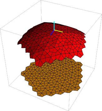
Figure 1: (Color online) Node set extracted from a 3D membrane network and its orthogonal projection onto the $x_{1},x_{2}$ plane.

3 Numerical results

3.1 Sinusoidal membrane

We begin by considering the node set ${X}_{N}$ such that $x_{a_{1}}$ and $x_{a_{2}}$ are randomly generated numbers within the interval $[0,\pi]$, and it results in $z_{a}=\sin(x_{a_{1}}^{2}+x_{a_{2}})$. Fig. 2 shows the LME surfaces ${S}_{N}$ obtained in this case for $N=500$, $\beta=0.001$, and $\beta=10$. The ${S}_{N}$ are sampled over a $12\times 12$ uniform grid of points defined over the $x_{1},x_{2}$ region $[0,\pi]\times[0,\pi]$. We observe from Fig. 2 that the ${S}_{N}$ corresponding to $\beta=0.001$ is almost flat, while the ${S}_{N}$ corresponding to $\beta=10$ fairly reproduces the local shape of ${X}_{N}$ in the neighborhood of each node.

Figure 2: (Color online) LME approximations of scattered data extracted from the sinusoidal surface ${S}:\ z=\sin({x_{1}}^{2}+x_{2})$ for two different values of $\beta$.

Next, we examine uniform grids of nodes ${\mathbf{x}}_{a}=\{x_{a_{1}},x_{a_{2}}\}$ over the $x_{1},x_{2}$ region $D=[0,3]\times[0,3]$, and the 3D node set ${X}_{N}=\{\hat{{\mathbf{x}}}_{a}=\{{\mathbf{x}}_{a},z_{a}=\sin(x_{a_{1}}^{2}+x_{a_{2}})\},\ a=1,...,N\}$. For each ${\mathbf{x}}_{a}\in D^{\prime}=[0.5,2.5]\times[0.5,2.5]\subset D$, we further consider the subset ${X}_{N}^{a}\subset{X}_{N}$, which is generated by the $m$th nearest neighbors of ${\mathbf{x}}_{a}$, $m$ being an integer parameter. We employ the node set ${X}_{N}^{a}$ to get LME estimates $H_{N}^{a}$ and $K_{N}^{a}$ of the mean and Gaussian curvatures of ${X}_{N}$ at $\hat{{\mathbf{x}}}_{a}$. In order to normalize the effects of $\beta$ on the LME estimates, we rescale such a parameter as follows

$$\beta\ =\ \frac{{\bar{\beta}}}{\left(\mbox{diam}({X}_{N}^{a})\right)^{2}}$$ (20)

where $\bar{\beta}$ is a dimensionless quantity and it results in

$$\mbox{diam}({X}_{N}^{a})\ =\ \max_{{\mathbf{x}}_{a},{\mathbf{x}}_{b}\in{X}_{N}^{a}}\{|{\mathbf{x}}_{a}-{\mathbf{x}}_{b}|\}.$$ (21)

It is useful to compare $H_{N}^{a}$ and $K_{N}^{a}$ with the ‘exact’ counterparts $H^{a}$ and $K^{a}$, which are easily computed through (18) and (19), by replacing $z_{N}$ with $z=\sin({x_{1}}^{2}+x_{2})$. The accuracy of the nodal LME estimates ${H}_{N}=\{H_{N}^{a},\ a=1,...,N^{\prime}\}$ and ${K}_{N}=\{K_{N}^{a},\ a=1,...,N^{\prime}\}$ can be inspected by examining the following Root Mean Square Deviations (RMSD)

$$\begin{array}[]{lll}RMSD({H}_{N})&=&\sqrt{\left(\sum^{N^{\prime}}_{a=1}{(H_{N}^{a}-H^{a})^{2}}\right)/N^{\prime}},\\ RMSD({K}_{N})&=&\sqrt{\left(\sum^{N^{\prime}}_{a=1}{(K_{N}^{a}-K^{a})^{2}}\right)/N^{\prime}}\end{array}$$ (22)

for different values of $\bar{\beta}$ and $m$. Here, $N^{\prime}$ denotes the total number of nodes belonging to $D^{\prime}$. We examine the following three different mesh sizes: $h=0.0566$ ($N=54\times 54$); $h=0.0405$ ($N=75\times 75$); and $h=0.0303$ ($N=100\times 100$). Here and in the following examples, we solve the nonlinear optimization problem (8) using recursive Newton-Raphson updates (9), up to the termination condition $|{\mathbf{r}}^{k}|<10^{-6}\ \mbox{diam}({X}_{N}^{a})$. Fig. 3 illustrates how the quantities $RMSD({H}_{N})$ and $RMSD({K}_{N})$ vary with $\bar{\beta}$ and $h$ for fixed $m=10$, while Figs. 4, 5 and 6 depict 2D and 3D density plots of the data sets ${H}_{N}$ and ${K}_{N}$ for several values of $m$, keeping $\bar{\beta}=150$, and $h=0.0303$ fixed. The results shown in Figures 4, 5 and 6 point out that the LME estimates ${H}_{N}$ and ${K}_{N}$ exhibit uniform asymptotic convergence to the exact solutions $H$ and $K$, respectively, for ${\bar{\beta}}\geq 100$, $m\geq 9$, and $h\leq 0.0303$.

Figure 3: (Color online) Root Mean Square Deviations (RMSD) of the LME approximations to the mean curvature $H$ and the Gaussian curvature $K$ of the sinusoidal surface $z=sin(x_{1}^{2}+x_{2})$ over the $x_{1},x_{2}$ domain $[0.5,2.5]\times[0.5,2.5]$. Left: RMSD as a function of $\bar{\beta}$, for $m=10$ and $h=0.0303$. Right: RMSD as a function of $h$, for $m=10$ and $\bar{\beta}=150$.

Figure 4: (Color online) 2D density plots of the LME approximations to the mean curvature $H$ of the sinusoidal surface $z=sin(x_{1}^{2}+x_{2})$ over the $x_{1},x_{2}$ domain $[0.5,2.5]\times[0.5,2.5]$, for $\bar{\beta}=150$, $h=0.0303$, and different values of $m$ (lower bound of the color bar: -4; .upper bound: +4).

Figure 5: (Color online) 2D density plots of the LME approximations to the Gaussian curvature $K$ of the sinusoidal surface $z=sin(x_{1}^{2}+x_{2})$ over the $x_{1},x_{2}$ domain $[0.5,2.5]\times[0.5,2.5]$, for $\bar{\beta}=150$, $h=0.0303$, and different values of $m$ (lower bound of the color bar: -0.56; upper bound: +0.56).

Figure 6: (Color online) 3D density plots of the LME approximations to the mean and the Gaussian curvatures of the sinusoidal surface $z=sin(x_{1}^{2}+x_{2})$ over the $x_{1},x_{2}$ domain $[0.5,2.5]\times[0.5,2.5]$, for $\bar{\beta}=150$, $h=0.0303$, and $m=12$.

3.2 Spherical membrane

We examine, in the present and the following sections, a closed membrane network ${X}_{N}$ corresponding to the CGMD model of the red blood cell given in (Marcelli et al.,, 2005; Hale et al.,, 2009). Such a model describes the system formed by the cytoskeleton spectrin network, the lipid bilayer and the transmembrane proteins of an actual RBC membrane, through a network of $N$ (virtual) particles embedded in a closed polyhedral surface showing $M$ triangular facets. Each particle has sixfold coordination, with the exception of twelve ‘defects,’ which instead have fivefold coordination. The particles represent discrete areas of the RBC membrane and their equilibrium distance $r_{0}$ is set equal to the average length of the spectrin filaments ($\sim$ 100 nm). Each particle has mass $m$ and is connected to it’s nearest neighbors though linear springs of stiffness $k$, which are parameterized such that the network of particles reproduces the membrane rigidity of a RBC. The bending rigidity is also accounted for by introducing dihedral angle potential energy terms of angular stiffness $D$ between adjacent triangles. The global surface area of the polyhedral membrane is kept constant using Lagrange multipliers, in order to mimic the relative incompressibility of the lipid bilayer of a normal RBC. The model under consideration is also able to keep the volume enveloped by the polyhedral membrane constant, with the aim to resemble the typical behaviour of a RBC in normal conditions. The dynamics of the RBC model can be obtained by integrating the Newton equations of motion of each virtual particle using a standard MD code. We used DL POLY 2.20((Smith and Forester,, 1999)), and employed the Nosé-Hoover thermostat; $6\times 10^{6}$ steps with time-step $\Delta t=2.07\times 10^{-5}\ t_{0}$, where $t_{0}=\sqrt{{m}/{k}}$; $N=5762$ particles; $m=5.82625\times 10^{-20}$ kg; $k=8.3\ \mu$N/m; $D=130\times 10^{-20}$ J; constant absolute temperature $T=309$ K; constant surface area $\bar{A}=4.986\times 10^{7}\ \mbox{nm}^{2}$; and constant volume $\bar{V}=3.311\times 10^{10}\ \mbox{nm}^{3}$. Such parameter settings allow the LME regularization to approximate a spherical surface ${S}$ with radius ${\bar{r}}=1992$ nm (Marcelli et al.,, 2005).

The theoretical average surface ${S}$ clearly has uniform principal curvatures $k_{1}=k_{2}=H=-1/{\bar{r}}=-5.019\times 10^{-4}\ \mbox{nm}^{-1}$ (the minus sign follows from the outward orientation of the normal vector), and Gaussian curvature $K=k_{1}k_{2}=25.19\times 10^{-8}\ \mbox{nm}^{-2}$. Nodal LME estimates ${H}_{N}=\{H_{N}^{a},\ a=1,...,N\}$ and ${K}_{N}=\{K_{N}^{a},\ a=1,...,N\}$ of the mean and Gaussian curvatures of the network can be obtained by introducing different local frames $\{\hat{{\mathbf{x}}}_{a},\ x_{1},\ x_{2},\ z\}$ at each different node $\hat{{\mathbf{x}}}_{a}$, with $x_{1}$, $x_{2}$ and $z$ tangent to the local parallel, meridian, and radial lines, respectively. Table 1 shows the mean values and the standard deviations of the data sets ${H}_{N}$ and ${K}_{N}$ defined as follows

$$\begin{array}[]{llllll}{\bar{H}}_{N}&=&1/N\ \sum^{N}_{a=1}{H_{N}^{a}},\ \ \ s_{d}({H}_{N})&=&\sqrt{\left(\sum^{N}_{a=1}{(H_{N}^{a}-{\bar{H}}_{N})^{2}}\right)/(N-1)}\end{array}$$ (23)

$$\begin{array}[]{llllll}{\bar{K}}_{N}&=&1/N\ \sum^{N}_{a=1}{K_{N}^{a}},\ \ \ s_{d}({K}_{N})&=&\sqrt{\left(\sum^{N}_{a=1}{(K_{N}^{a}-{\bar{K}}_{N})^{2}}\right)/(N-1)}\end{array}$$ (24)

for $\bar{\beta}=100$ and different values of $m$. The results in Table 1 highlight a good agreement between LSM estimates and exact solutions for $m\geq 10$. It has to be considered that the MD model doesn’t reach a perfectly (average) spherical shape at equilibrium, due to the presence of the fivefold defects.

	$m=5$	$m=7$	$m=9$	$m=10$	$m=12$
${\bar{H}}_{N}\times 10^{5}\ \mbox{\AA}^{-1}$	39.0626	-7.1062	-5.1293	-5.0443	-5.0311
$s_{d}({H}_{N})\times 10^{5}\ \mbox{\AA}^{-1}$	2.8047	0.1467	0.0296	0.0271	0.0238
${\bar{K}}_{N}\times 10^{10}\ \mbox{\AA}^{-2}$	1540.19	50.488	26.3077	25.4453	25.3118
$s_{d}({K}_{N})\times 10^{10}\ \mbox{\AA}^{-2}$	234.04	2.1551	0.3152	0.2840	0.2473

Table 1: Mean and standard deviation of the data sets ${H}_{N}$ and ${K}_{N}$ for a spherical membrane network with $N=5762$ nodes and radius $r=1992\ \mbox{nm}$, considering $\bar{\beta}=100$ and different values of $m$. Exact solution: $H=-5.019\times 10^{-5}\ \mbox{\AA}^{-1}$, $K=25.19\times 10^{-10}\ \mbox{\AA}^{-2}$.

3.3 Principal curvatures of the RBC membrane

We analyze in the present section a slight different formulation of the RBC model given in (Marcelli et al.,, 2005; Hale et al.,, 2009), which differs from that discussed in the previous section only in terms of the volume constraint. Here, we set the volume enveloped by the RBC membrane equal to 0.65 times the volume of the sphere analyzed in the previous example, allowing the current model to assume the typical biconcave shape of a normal RBC (Hale et al.,, 2009).The surface area of the RBC membrane is again set to $4.986\times 10^{7}\ \mbox{nm}^{2}$, as in the previous case. We compute nodal LME estimates ${H}_{N}=\{H_{N}^{a},\ a=1,...,N\}$ and ${K}_{N}=\{K_{N}^{a},\ a=1,...,N\}$ of the mean and Gaussian curvatures of a real RBC membrane by processing the rolling average configurations ${X}_{N}$ of the CGMD model up to different simulation times $t$. Let $n$ denote the weighted unit normal to the current vertex $\hat{{\mathbf{x}}}_{a}$ of the triangulation associated with ${X}_{N}$, assuming the triangle areas as the weights (Taubin,, 1995). In the present case, we define the local $x_{1}$ axis as the direction of the edge attached to $\hat{{\mathbf{x}}}_{a}$ that has the minimum deviation from the parallel drawn on an ideal sphere passing through the same point. In addition, we define $x_{2}$ by means of the vector product of the unit vectors in the directions of $n$ and $x_{1}$, and $z$ via the vector product of the unit vectors in the directions of $x_{1}$ and $x_{2}$. A graphical representation of the local parameterization introduced for the analyzed model of the RBC membrane is provided in Fig. 7.

Figure 7: (Color online) 3D map of the local bases $\{\hat{{\mathbf{x}}}_{a},\ x_{1},\ x_{2},\ z\}$ introduced at selected nodes of a triangulated model of the RBC membrane ($x_{1}$: yellow, $x_{2}$: blue, $z$: cyan) .

Fig. 8 shows the dependence of the LME estimates ${\bar{H}}_{N}$ and ${K}_{N}^{tot}={\bar{K}}_{N}{\bar{A}}$ on $\bar{\beta}$, for $t=75.5\ t_{0}$ and $m=10$. It is worth noting that ${K}_{N}^{tot}$ represents an estimate of the total curvature ${K}^{tot}=\int_{S_{N}}K\ dA$ of the RBC model. Due to the ‘Gauss-Bonet theorem’ such a quantity only depends on the genus of $S_{N}$ and should be equal to $4\pi$, as in the case of a sphere (Stoker,, 1969). One observes from Fig. 8 slight oscillations of ${\bar{H}}_{N}$ and ${K}_{N}^{tot}$ with $\bar{\beta}$; ${K}_{N}^{tot}/4\approx 3.00$ for $\bar{\beta}<100$; and ${K}_{N}^{tot}/4\approx 3.14$ for $\bar{\beta}=125$. 3D density plots of the data sets ${H}_{N}$ and ${K}_{N}$ are given in Figs. 9 and 10, considering $\bar{\beta}=125$, $m=10$, and different simulation times $t$. The results shown in Figs. 9 and 10 indicate that the LME regularizations of the average CGMD configurations smoothly describe the geometry of a normal RBC membrane. The LME regularization is indeed able to reproduce the biconcave shape of such a membrane (consider that the hidden bottom edges of the surfaces shown in Figs. 9 and 10 are nearly specular with respect to the top ones), furnishing positive (red) and negative (blue) mean curvatures in correspondence with concave and convex portions, respectively (cf. Fig. 9), and negative (blue) Gaussian curvatures over saddle-shaped regions (cf. Fig. 10). One observes perturbations in the mean and Gaussian curvature maps in correspondence with the fivefold defects of the membrane triangulation during the initial phase of the MD simulation. The MD simulation and the LME regularization are however able to smooth out the local noise produced by such perturbations, as the simulation time progressively increases.

Figure 8: (Color online) LME estimates $|{\hat{\bar{H}}}_{N}|=|{\bar{H}}_{N}|\times 10^{5}\ \mbox{\AA}^{-1}$ and ${K}_{N}^{tot}$ for a CGMD model of the RBC membrane Marcelli et al., (2005); Hale et al., (2009), considering different values of $\bar{\beta}$, $m=10$, and $t=75.5\ t_{0}$.

Figure 9: (Color online) 3D density plots of the LME approximations ${H}_{N}$ to the mean curvature $H$ of of a CGMD model of the RBC membrane Marcelli et al., (2005); Hale et al., (2009) at different simulation times $t$, for $\bar{\beta}=125$ and $m=10$ (${\hat{\bar{H}}}_{N}={\bar{H}}_{N}\times 10^{5}\ \mbox{\AA}^{-1}$; lower bound of the color bar: $-11.5\times 10^{-5}\ \mbox{\AA}^{-1}$; upper bound: $+2.5\times 10^{-5}\ \mbox{\AA}^{-1}$).

Figure 10: (Color online) 3D density plots of the LME approximations ${K}_{N}$ to the Gaussian curvature $K$ of of a CGMD model of the RBC membrane Marcelli et al., (2005); Hale et al., (2009) at different simulation times $t$, for $\bar{\beta}=125$ and $m=10$ (lower bound of the color bar: $-2\times 10^{-9}\ \mbox{\AA}^{-2}$; upper bound: $+7\times 10^{-9}\ \mbox{\AA}^{-2}$).

3.4 Estimation of the bending rigidity of membrane networks from MD simulations

Let us consider now a triangulated membrane network endowed with the following dihedral angle energy

$$\begin{split}E^{\rm dihedral}&=D\sum_{\triangle,\triangle^{\prime}\in{\cal C}_{\triangle}\atop\text{neighbors}}\left(1-\cos\widehat{\triangle\triangle^{\prime}}\right)\ =\ \frac{D}{2}\sum_{\triangle,\triangle^{\prime}\in{\cal C}_{\triangle}\atop\text{neighbors}}|n_{\triangle}-n_{\triangle^{\prime}}|^{2}\end{split}$$ (25)

where ${\cal C}_{\triangle}$ denotes the set of all triangles forming the network; $\widehat{\triangle\triangle^{\prime}}$ is the dihedral angle between the triangles $\triangle$ and $\triangle^{\prime}$; $n_{\triangle}$ is the unit normal to the triangle $\triangle$; and the summation runs over all the pairs $\triangle,\triangle^{\prime}\in{\cal C}_{\triangle}$ which share a common side. According to (Seung and Nelson,, 1988; Gompper and Kroll,, 1996), the limiting bending energy of such a network is a Helfrich-type bending energy (Deuling and Helfrich,, 1976) of the form

$$E^{{bend}}\ =\ \frac{\kappa_{H}}{2}\ \int_{S_{N}}((2H)^{2}\ -\ 2K)\ dS$$ (26)

where $\kappa_{H}$ is the bending rigidity, and it results $\kappa_{H}=\sqrt{3}D/3$ for a sphere, and $\kappa_{H}=\sqrt{3}D/2$ for a cylinder (Gompper and Kroll,, 1996) (Note that in (Seung and Nelson,, 1988; Gompper and Kroll,, 1996) the symbol $H$ is used to denote twice the mean curvature of the network).

The LME prediction of the principal curvatures of the network allows us to estimate the limiting bending energy (26). As a matter of fact, the computing of the mean curvatures ${H}_{N}=\{H_{N}^{a},\ a=1,...,N\}$ of the current configuration leads us to approximate (26) as follows

$$E_{N}^{{\rm bend}}\ =\ \frac{\kappa_{H}}{2}\ \left[\left(\sum_{a=1}^{N}\ (2H_{N}^{a})^{2}A_{N}^{a}\right)\ -\ 8\pi\right]$$ (27)

where $A_{N}^{a}$ is the surface area of the $a$-th element of a dual tessellation of the network, which we assume is formed by polygons joining the midpoints of the network edges with the triangle barycenters (barycentric dual mesh). Equation (27) can be employed to estimate the bending modulus at zero temperature of the network, through the Cauchy-Born contribution (Ericksen,, 2008; Zhou and Joós,, 1996) to the isothermal bending rigidity, here denoted by $\kappa_{H}^{0}$. The latter consists of the configurational average of the instantaneous bending rigidities of the fluctuating network. On matching $E_{N}^{{\rm bend}}$ to $E^{{\rm dihedral}}$ (energetic discrete-to-continuum approach), we identify the instantaneous bending rigidity with the ratio $E^{\rm dihedral}/\left.\left(E_{N}^{\rm bend}\right)\right|_{\kappa_{H}=1}$ , and compute $\kappa_{H}^{0}$ through

$$\kappa_{H}^{0}\ =\ \left\langle\frac{E^{{\rm dihedral}}}{\left.\left(E_{N}^{\rm bend}\right)\right|_{\kappa_{H}=1}}\right\rangle$$ (28)

where $\langle\cdot\rangle$ denotes the configurational average symbol.

For the sake of example, let us reconsider now the MD model of the RBC membrane examined in the previous section. Fig. 11 shows the time history that we obtained for the zero-temperature bending rigidity $\kappa_{H}^{0}$ of such a model, on computing the rolling averages of the quantity ${2\ E^{{\rm dihedral}}}/{E_{N}^{{\rm bend}}}$ during a MD simulation (cf. Sect. 3.3). It is seen from Fig. 11 that the value of $\kappa_{H}^{0}$ slightly fluctuates during the simulation, featuring oscillations with progressively smaller amplitude as the computational time $t$ increases. We estimated a limiting value of $\kappa_{H}^{0}$ approximatively equal to 79 J, for $t>100\ t_{0}$. Such a value is just slightly greater than that predicted in (Gompper and Kroll,, 1996) for the sphere ($\sqrt{3}D/3=75.06$ J), which is not surprising, since the biconcave (average) shape of the RBC model under consideration has the same genus of the sphere.

Figure 11: LME estimates of the zero-temperature bending rigidity of the RBC membrane model presented in Section 3.3, at different times of a MD simulation.

4 Concluding remarks

We have presented and numerically tested a meshfree approach to the curvature and bending rigidity estimation of membrane networks, through a suitable extension of the LME method formulated in (Arroyo and Ortiz,, 2006). The results of Sections 3.1 and 3.2 demonstrate the convergence properties of the LME curvature estimates, both for a rectangular geometry (fixed $\{x_{1},x_{2},z\}$ axes), and for a spherical membrane. On the other hand, the results presented in Sections 3.3 and 3.4, emphasize the ability of the LME approach in tracking the local curvatures and the bending rigidity of the RBC model presented in (Marcelli et al.,, 2005). Concerning the parameter estimation, we have found that the limitations $\bar{\beta}\geq 100$ and $m\geq 10$ generally ensure stable curvature predictions. In particular, for $m\geq 10$ we found that100 is approximately the smallest value of $\bar{\beta}$ that guarantees asymptotic convergence of LME curvature predictions for the examined examples. The value of $\bar{\beta}$ rules the degree of locality of LME approximations, which reduce to piecewise affine shape functions supported by a Delaunay triangulation for $\bar{\beta}\rightarrow\infty$ (Arroyo and Ortiz,, 2006; Cyron et al.,, 2009).

In closing, we suggest some directions for relevant extensions of the present work. We intend to apply the LME regularization algorithm to predict the entire set of the isothermal membrane and bending rigidities of fluctuating biomembranes modeled through MD simulations, with special reference to the RBC membrane. We plan to combine the LME regularization of the RBC model proposed in (Marcelli et al.,, 2005), with the elastic moduli estimation procedures given in (Seung and Nelson,, 1988; Gompper and Kroll,, 1996; Zhou and Joós,, 1996). Another application of the LME procedure presented in this work is to mesure the curvature of lipid bilayers as modelled with MD simulations. Lipid bilayers are generally flat, however several different protein-driven processes will result in the membrane curvature that is required for various cell processes (i.e. fusion). One mechanism is caused by protein domains inserting shallowly into one of the lipid leaflets, which push the neighboring lipid head groups away and therefore causing local spontaneous curvature. We are currently conducting coarse-grain MD simulations that model the interactions between different varieties of these protein domains and lipid bilayers. The LME procedure will allow us to quantify the amount of curvature that results from these interactions.

References

- Arroyo and Ortiz, (2006) Arroyo, M. and Ortiz, M. (2006). Local maximum-entropy approximation schemes: a seamless bridge between finite elements and meshfree methods. Int. J. Numer. Meth. Eng., 65(13):2167–2202.
- Cyron et al., (2009) Cyron, C., Arrojo, M., and M., O. (2009). Smooth, second-order, non-negative meshfree approximants selected by maximum entropy. Int. J. Num. Meth. Enging., 79:1605–1632.
- Dao et al., (2006) Dao, M., Li, J., and Suresh, S. (2006). Molecularly based analysis of deformation of spectrin network and human erythrocyte. Mat. Sci. Engng., 26:1232–1244.
- Deuling and Helfrich, (1976) Deuling, H. and Helfrich, W. (1976). Red blood cell shapes as explained on the basis of curvature elasticity. Biophys J., 16(8):861–868.
- Du et al., (2006) Du, Q., Liu, C., and Wang, X. (2006). Simulating the deformation of vescicle membranes under elastic bending energy in three dimensions. J. Comput. Phys., 212:756–777.
- Ericksen, (2008) Ericksen, J. (2008). On the cauchy-born rule. Math. Mech. Solids, 13:199–220.
- Gompper and Kroll, (1996) Gompper, G. and Kroll, D. (1996). Random surface discretization and the renormalization of the bending rigidity. J. Phys. I France, 6:1305–1320.
- Hale et al., (2009) Hale, J., Marcelli, G., Parker, K., Winlowe, C., and Petrov, G. (2009). Red blood cell thermal fluctuations: comparison between experiment and molecular dynamics simulations. Soft Matter, 5:3603–3606.
- Jaines, (1957) Jaines, E. (1957). Information theory and statistical mechanics. Phis. Rev., 106:620–630.
- Li et al., (2010) Li, B., Habbal, F., and Ortiz, M. (2010). Optimal transportation meshfree approximation schemes for fluid and plastic flows. Int. J. Num. Meth. Enging.
- Marcelli et al., (2005) Marcelli, G., Parker, H., and Winlove, P. (2005). Thermal fluctuations of red blood cell membrane via a constant-area particle-dynamics model. Biophys. J., 89:2473–2480.
- Martens and McMahon, (2008) Martens, S. and McMahon, H. (2008). Mechanisms of membrane fusion: disparate players and common principles. Nature Rev., 9:543–556.
- McMahon and Gallop, (2005) McMahon, H. and Gallop, J. (2005). Membrane curvature and mechanisms of dynamic cell membrane remodelling. Nature, 438:590–596.
- Naghdi, (1972) Naghdi, P. (1972). The theory of shells and plates. In Trusdell, C., editor, S. Flügge’s Handbuch der Physik, volume VIa/2, pages 425–640. Springer Verlag.
- Rajan, (1994) Rajan, V. (1994). Optimality of the delunay triangulation in . Discrete Comput. Geom., 12(2):189–202.
- Risselada and Marrink, (2009) Risselada, H. J. and Marrink, S. (2009). Curvature effects on lipid packing and dynamics in liposomes revealed by coarse grained molecular dynamics simulations. Phys. Chem., 11:2056–2067.
- Seung and Nelson, (1988) Seung, H. and Nelson, D. (1988). Defects in flexible membranes with crystalline order. Phys. Rev. A, 38:1005–1018.
- Smith and Forester, (1999) Smith, W. and Forester, T. (1999). The dl_poly_2 molecular simulation package. http://www.cse.clrc.ac.uk/msi/software/DL_POLY.
- Stoker, (1969) Stoker, J. J. (1969). Differential Geometry. Wiley, New York.
- Taubin, (1995) Taubin, G. (1995). Estimating the tensor of curvature of a surface from a polyhedral approximation. In Proc. 5th Intl. Conf. on Computer Vision (ICCV95), pages 902–907.
- Zhou and Joós, (1996) Zhou, Z. and Joós, B. (1996). Stability criteria for homogeneously stressed materials and the calculation of elastic constants. Phys. Rev. B, 54(6):3841–3850.