A Godunov-type method for the shallow water equations with discontinuous topography in the resonant regime

Abstract

We investigate the Riemann problem for the shallow water equations with variable and (possibly) discontinuous topography and provide a complete description of the properties of its solutions: existence; uniqueness in the non-resonant regime; multiple solutions in the resonant regime. This analysis leads us to a numerical algorithm that provides one with a Riemann solver. Next, we introduce a Godunov-type scheme based on this Riemann solver, which is well-balanced and of quasi-conservative form. Finally, we present numerical experiments which demonstrate the convergence of the proposed scheme even in the resonance regime, except in the limiting situation when Riemann data precisely belong to the resonance hypersurface.

1 Introduction

In this paper we design a Godunov-type scheme for the numerical approximation of weak solutions to the initial-value problem associated with the shallow water equations with variable topography, i.e.

$$\begin{array}[]{ll}&\partial_{t}h+\partial_{x}(hu)=0,\\ &\partial_{t}(hu)+\partial_{x}\Big{(}h(u^{2}+{gh\over 2})\Big{)}+gh\,\partial_{x}a=0,\\ \end{array}$$ (1.1)

where the height of the water from the bottom to the surface, denoted by $h$, and the fluid velocity $u$ are the main unknowns. Here, $g$ is the so-called gravity constant, and $a=a(x)$ (with $x\in{R\!\!\!\!\!I~{}}$) is the height of the bottom from a given level.

In [27], LeFloch pointed out that by supplementing balance laws like (1.1) with the additional equation

$$\partial_{t}a=0,$$ (1.2)

the set of equations (1.1)–(1.2) can be regarded as a nonlinear hyperbolic system in nonconservative form and tackled with the theory introduced by Dal Maso, LeFloch, and Murat [12] and developed by LeFloch and collaborators [26, 30, 19, 10]. As is well-known, the system (1.1)–(1.2) is hyperbolic but not strictly hyperbolic since characteristic speeds may coincide on certain hypersurfaces. Non-strictly hyperbolic systems have been extensively studied in the literature. See [27, 34, 32, 37] for the model of fluid flows in a nozzle with variable cross-section, [21, 20, 15, 3, 4] for other models.

On the other hand, the discretization of source terms in nonlinear hyperbolic balance laws like the shallow water equations was pioneered by Greenberg and Leroux [17]. We built here on this paper as well as the follow-up work [1, 9, 8, 11, 16, 18, 22, 23]. Since the system (1.1) is also related to the class of two-phase models, we are also motivated by the existing research work on the discretization of two-phase flow models [2, 4, 14]. In particular, recall that well-balanced schemes for shallow water equations were constructed first in [14, 17, 22, 23]. In addition, the discretization of nonconservative hyperbolic systems and of systems with source terms attracted a lot of attention in recent years. We refer to [5, 6, 7, 16, 18] for a single conservation law with source term and to [22, 23, 25, 24] for fluid flows in a nozzle with variable cross-section. Well-balanced schemes for multi-phase flows and other models were studied in [2, 9, 36, 38].

The Godunov scheme is based on an exact or approximate Riemann solver and, consequently, it is necessary that sufficient information be available on the existence and properties of all solutions to (1.1)–(1.3). Recall that the Riemann problem is a Cauchy problem with piecewise constant initial data of the form

$$(h,u,a)(x,0)=\left\{\begin{array}[]{ll}(h_{L},u_{L},a_{L}),&x<0,\\ (h_{R},u_{R},a_{R}),&x>0.\end{array}\right.$$ (1.3)

One main task in the present paper will be to revisit the construction of solutions to the Riemann problem for (1.1)–(1.3) in order to arrive at a definite algorithm for their numerical computation. We will show that a unique solution exists within a large domain of initial data, and will precisely identify the domains where multiple solutions are available, by providing necessary and sufficient conditions for the existence of multiple (up to three) solutions.

Recall that, in LeFloch and Thanh [33], a first investigation of the Riemann problem for the shallow water equations was performed. The present paper provides a very significant improvement in that a complete description of a Riemann solver is now obtained for the first time. We are able to distinguish between cases of existence, uniqueness, and multiplicity of solutions.

We refer the reader to [1, 8, 35] for partial or alternative approaches to the Riemann problem. On the other hand, Chinnayya, LeRoux, and Seguin [11] introduced a Godunov method for (1.1) based on a Riemann solver determined by “continuation”: they start their construction by assuming that the bottom topography is flat and then extend it to a non-flat topography. Their method allows them to construct solutions within the regime where the nonlinear characteristic fields are separated by the linearly degenerate one, that is, the case where one wave speed is negative and the other positive. In this regime, the Riemann solution with non-flat bottom can be obtained from the the wave curves associated with the fast wave family, only, and these two waves are separated by a stationary wave. In particular, the total number of waves in Riemann solutions is exactly the number of characteristic families. On the other hand, when more general Riemann data are considered and lie in the other two strictly hyperbolic regions, say of “cross-region” type, we find it hard to apply this method. There is always a major difference between the “flat-bottom” and “non-flat-bottom” cases, since in one case the system is strictly hyperbolic, the other case the system is not strictly hyperbolic. Indeed, in the non-flat-bottom case, new wave curves arise that replace more standard wave curves. The total number of waves in a solution can possibly be larger than the number of characteristic fields as waves associated with a given family can be repeated. The appearance of such new wave curves cannot be obtained by a continuation argument.

Our objective in the present work is to present a numerical algorithm that provides an explicit construction of a Riemann solver for the shallow water equations in the resonant or non-resonant regimes. This solver then provides us with solutions to local Riemann problems which we can use to design a Godunov-type scheme. We also provide extensive numerical experiments and, within strictly hyperbolic regions of the phase space, our tests demonstrate that the proposed scheme converge to the expected solution. In resonance regions, we also observe convergence, except when the Godunov scheme takes some values on the resonance hypersurfaces. The Godunov scheme proposed in the present paper for (1.1)–(1.2) turns out to be well-balanced and captures exactly stationary waves.

This paper is organized as follows. In Section 2, we recall basic facts about the system (1.1)–(1.2) and provide the computing algorithm for stationary contact waves. In Section 3, we revisit the construction of solutions to the Riemann problem, and present a new approach based on a “gluing” technique involving different solution structures. With this technique, we establish the existence of solutions for arbitrary large initial data. In Section 4 we then present our computing strategy leading to a Riemann solver and, finally, are in a position to design a corresponding Godunov scheme. Section 5 is devoted to numerical experiments when data belong to strictly hyperbolic domains; in particular, we estimate the numerical errors and observe convergence when the mesh size tends to zero. Finally, Section 6 is devoted to numerical tests here data belong to resonance regions, and precisely identify regimes of convergence or non-convergence.

2 Shallow water equations

2.1 Wave curves

Introducing the dependent variable $(h,u,a)=(h,u,a)(x,t)$, the Jacobian matrix of the system (1.1)–(1.2) admits three real eigenvalues, i.e.

$$\lambda_{1}(U):=u-\sqrt{gh}<\lambda_{2}(U):=u+\sqrt{gh},\quad\lambda_{3}(U):=0,$$ (2.1)

together with the corresponding eigenvectors:

$$r_{1}(U):=\left(\begin{matrix}h\\ -\sqrt{gh}\\ 0\end{matrix}\right),\quad r_{2}(U):=\left(\begin{matrix}h\\ \sqrt{gh}\\ 0\end{matrix}\right),\quad r_{3}(U):=\left(\begin{matrix}gh\\ -gu\\ u^{2}-gh\end{matrix}\right),$$ (2.2)

so that the system (1.1)–(1.2) is hyperbolic, but not strictly hyperbolic. More precisely, the first and the third characteristic speeds coincide,

$$(\lambda_{1}(U),r_{1}(U))=(l_{3}(U),r_{3}(U)),$$

on the hypersurface

$$\mathcal{C}_{+}:=\Big{\{}(h,u,a)|\quad u=\sqrt{gh}\Big{\}}.$$ (2.3)

The second and the third characteristic fields coincide,

$$(\lambda_{2}(U),r_{2}(U))=(\lambda_{3}(U),r_{3}(U)),$$

on the hypersurface

$$\mathcal{C}_{-}:=\Big{\{}(h,u,a)|\quad u=-\sqrt{gh}\Big{\}}.$$ (2.4)

In the following, we introduce $\mathcal{C}:=\mathcal{C}_{+}\cup\mathcal{C}_{-}$, and we refer to the sets $\mathcal{C}_{\pm}$ as the resonance hypersurfaces, which separate the phase space in the $(h,u,a)$-variable into three sub-domains

$$\begin{array}[]{ll}&G_{1}:=\Big{\{}(h,u,a)\in{R\!\!\!\!\!I~{}}_{+}\times{R\!\!\!\!\!I~{}}\times{R\!\!\!\!\!I~{}}_{+}|\quad\lambda_{1}(U)>\lambda_{3}(U)\Big{\}},\\ &G_{2}:=\Big{\{}(h,u,a)\in{R\!\!\!\!\!I~{}}_{+}\times{R\!\!\!\!\!I~{}}\times{R\!\!\!\!\!I~{}}_{+}|\quad\lambda_{2}(U)>\lambda_{3}(U)>\lambda_{1}(U)\Big{\}},\\ &G_{3}:=\Big{\{}(h,u,a)\in{R\!\!\!\!\!I~{}}_{+}\times{R\!\!\!\!\!I~{}}\times{R\!\!\!\!\!I~{}}_{+}|\quad\lambda_{3}(U)>\lambda_{2}(U)\Big{\}},\end{array}$$ (2.5)

in which the system is strictly hyperbolic. It is convenient to also set

$$G_{2}^{+}:=\{(h,u,a)\in G_{2},u\geq 0\},\qquad G_{2}^{-}:=\{(h,u,a)\in G_{2},u\leq 0\}.$$

Observe that for $u\geq 0$, the set $G_{1}$ is referred to as the domain of supercritical flows, where the Froude number

$$Fr:={u\over\sqrt{gh}}$$

is larger than 1, and the set $G_{2}^{+}$ as the domain of subcritical flows, where $Fr<1$. This concept may similarly be extended to the case $u<0$. See Figure 1.

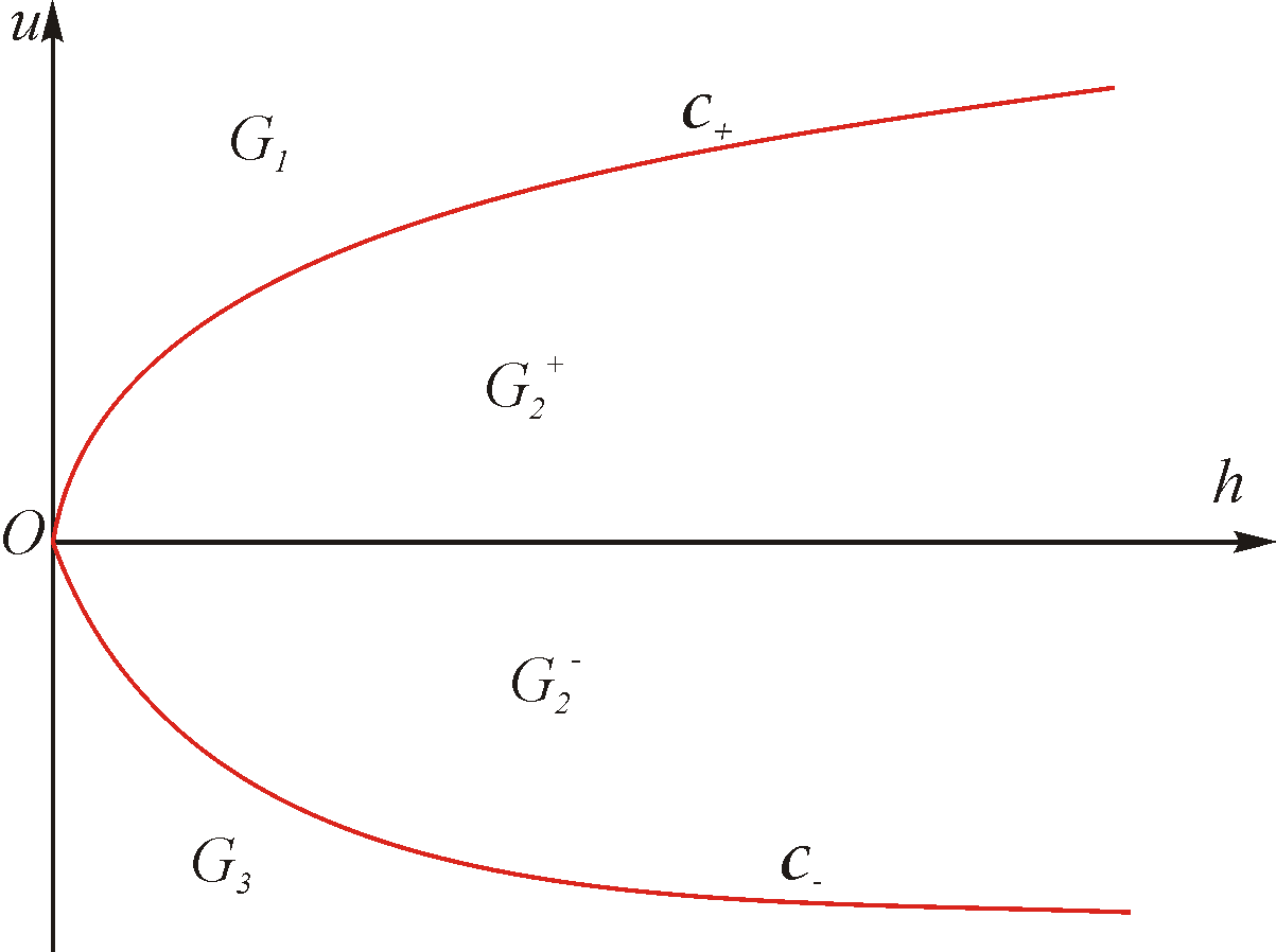
Figure 1: Phase domain in the $(h,u)$-plane.

One easily checked that the first and second characteristic fields $(\lambda_{1},r_{1})$, $(\lambda_{2},r_{2})$ are genuinely nonlinear, while the third characteristic field $(\lambda_{3},r_{3})$ is linearly degenerate.

As discussed in [33], across a discontinuity there are two possibilities:

• either the bottom height $a$ remains constant,

• or the discontinuity is stationary (i.e. propagates with zero speed).

In the first the case (i), the system (1.1)–(1.2) reduces to the standard shallow water equations with flat bottom. We can determine the $i$-shock curve $\mathcal{S}_{i}(U_{0})$ starting from a left-hand state $U_{0}$ and consisting of all right-hand states $U$ that can be connected to $U_{0}$ by a Lax shock associated with the first characteristic field ($i=1,2$):

$$\mathcal{S}_{i}(U_{0}):\quad\Psi_{i}(U;U_{0}):=u-u_{0}\pm\sqrt{g\over 2}(h-h_{0})\sqrt{\Big{(}{1\over h}+{1\over h_{0}}\Big{)}}=0.$$ (2.6)

where $U=(h,u)$, $h>h_{0}$ for $i=1$ and $\quad h<h_{0}$ for $i=2$. We also define the backward $i$-shock curve $\mathcal{S}_{i}^{B}(U_{0})$ starting from a right-hand state $U_{0}$ and consisting of all left-hand states $U$ that can be connected to $U_{0}$ by a Lax shock associated with the first characteristic field $(i=1,2$):

$$\mathcal{S}_{i}^{B}(U_{0}):\quad\Phi_{i}(U;U_{0}):=u-u_{0}\pm\sqrt{g\over 2}(h-h_{0})\sqrt{\Big{(}{1\over h}+{1\over h_{0}}\Big{)}}=0,$$ (2.7)

where $U=(h,u)$, $h<h_{0}$ for $i=1$ and $\quad h>h_{0}$ for $i=2$.

It is interesting that the shock speed of the nonlinear characteristic fields may coincide with the speed of stationary contact waves. The following lemma is easily checked.

Lemma 2.1.

Consider the projection on the $(h,u)$-plan. To every $U=(h,u)\in G_{1}$ there exists exactly one point $U^{\#}\in\mathcal{S}_{1}(U)\cap G_{2}^{+}$ such that the $1$-shock speed $\bar{\lambda}_{1}(U,U^{\#})=0$. The state $U^{\#}=(h^{\#},u^{\#})$ is defined by

$$h^{\#}=\frac{-h+\sqrt{h^{2}+8hu^{2}/g}}{2},\quad u^{\#}=\frac{uh}{h^{\#}}.$$

Moreover, for any $V\in\mathcal{S}_{1}(U)$, the shock speed $\bar{\lambda}_{1}(U,V)>0$ if and only if $V$ is located above $U^{\#}$ on $\mathcal{S}_{1}(U)$.

It is also well-known that the bottom height $a$ remains constant through rarefaction fans. The forward rarefaction curve $\mathcal{R}_{i}(U_{0})$ starting from a given left-hand state $U_{0}$ and consisting of all the right-hand states $U$ that can be connected to $U_{0}$ by a rarefaction wave associate with the first characteristic field as

$$\mathcal{R}_{i}(U_{0}):\quad\Psi_{i}(U;U_{0})=u-u_{0}\pm 2\sqrt{g}(\sqrt{h}-\sqrt{h_{0}})=0,\quad i=1,2,$$ (2.8)

where $U=(h,u),h\leq h_{0}$ for $i=1$ and $h\geq h_{0}$ for $i=2$. Given a right-hand state $U_{0}$, the backward $i$-rarefaction curve $\mathcal{R}_{i}^{B}(U_{0})$ consisting of all left-hand states $U$ that can be connected to $U_{0}$ by a rarefaction wave associated with the first characteristic field reads $(i=1,2$)

$$\mathcal{R}_{i}^{B}(U_{0}):\quad\Phi_{i}(U;U_{0})=u-u_{0}\pm 2\sqrt{g}(\sqrt{h}-\sqrt{h_{0}})=0,$$ (2.9)

where $U=(h,u),h\geq h_{0}$ for $i=1$ and $h\leq h_{0}$ for $i=2$.

Finally, we define the forward and backward wave curves in the $(h,u)$-plane $(i=1,2$):

$$\begin{array}[]{ll}&\mathcal{W}_{i}(U_{0}):=\mathcal{S}_{i}(U_{0})\cup\mathcal{R}_{i}(U_{0})=\{U\ |\ \Psi_{i}(U;U_{0})=0\},\\ &\mathcal{W}_{i}^{B}(U_{0}):=\mathcal{S}_{i}^{B}(U_{0})\cup\mathcal{R}_{i}^{B}(U_{0})=\{U\ |\ \Phi_{i}(U;U_{0})=0\}.\end{array}$$ (2.10)

It is checked in [33] that the wave curves $\mathcal{W}_{1}(U_{0})$ and $\mathcal{W}_{1}^{B}(U_{0})$ parameterized as $h\mapsto u=u(h),h>0,$ are strictly convex and strictly decreasing functions. The wave curve $\mathcal{W}_{2}(U_{0})$ and $\mathcal{W}_{2}^{B}(U_{0})$ being parameterized as $h\mapsto u=u(h),h>0,$ are strictly concave and strictly decreasing functions.

In the case (ii), the discontinuity satisfies the jump relations

$$\begin{array}[]{ll}&[hu]=0,\\ &[{u^{2}\over 2}+g(h+a)]=0,\\ \end{array}$$ (2.11)

which determine the stationary-wave curve (parameterized with $h$):

$$\begin{array}[]{ll}\mathcal{W}_{3}(U_{0}):&u=u(h)={h_{0}u_{0}\over h},\\ &a=a(h)=a_{0}+{u_{0}^{2}-u^{2}\over 2g}+h_{0}-h.\end{array}$$ (2.12)

The projection of the wave curve $\mathcal{W}_{3}(U_{0})$ in the $(h,u)$-plane can be parameterized as $h\mapsto u=u(h),h>0,$ which is a strictly convex and strictly decreasing function for $u_{0}>0$ and strictly concave and strictly increasing function for $u_{0}<0$.

The above arguments show that the $a$-component of Riemann solutions may change only across a stationary wave. This property will be important later when designing the discretization of the source terms.

2.2 Properties of stationary contacts

Given a state $U_{0}=(h_{0},u_{0},a_{0})$ and another bottom level $a\neq a_{0}$, we let $U=(h,u,a)$ be the corresponding right-hand state of the stationary contact issuing from the given left-hand state $U_{0}$. We now determine $h,u$ in terms of $U_{0},a$, as follows. Substituting $u=h_{0}u_{0}/h$ from the first equation of (2.12) to the second equation of (2.12), we obtain

$$a_{0}+{1\over 2g}\left(u_{0}^{2}-\left({h_{0}u_{0}\over h}\right)^{2}\right)+h_{0}-h=a.$$

Multiplying both sides of the last equation by $2gh^{2}$, and then re-arranging terms, we find that $h>0$ is a root of the nonlinear equation

$$\varphi(h) =\varphi(U_{0},a;h)$$ (2.13)

$$:=2gh^{3}+(2g(a-a_{0}-h_{0})-u_{0}^{2})h^{2}+h_{0}^{2}u_{0}^{2}=0.$$

We easily check

$$\begin{array}[]{ll}&\varphi(0)=h_{0}^{2}u_{0}^{2}\geq 0,\\ &\varphi^{\prime}(h)=6gh^{2}+2(2g(a-a_{0}-h_{0})-u_{0}^{2})h,\\ &\varphi^{\prime\prime}(h)=12gh+2(2g(a-a_{0}-h_{0})-u_{0}^{2}),\end{array}$$

so that

$$\varphi^{\prime}(h)=0 \textrm{iff}\quad h=0$$ (2.14)

$$\textrm{or}\quad h=h_{*}=h_{*}(U_{0},a):=\frac{u_{0}^{2}+2g(a_{0}+h_{0}-a)}{3g}.$$

If $h_{*}(U_{0},a)<0$, or $a>a_{0}+h_{0}+{u_{0}^{2}\over 2g},$ then $\varphi^{\prime}(h)>0$ for $h>0$. Since $\varphi(0)=h_{0}^{2}u_{0}^{2}\geq 0$, there is no root for (2.13) if (2.14) holds. Otherwise, if

$$a\leq a_{0}+h_{0}+{u_{0}^{2}\over 2g},$$

then $\varphi^{\prime}>0$ for $h>h_{*}$ and $\varphi^{\prime}(h)<0$ for $0<h<h_{*}$. In this case, $\varphi$ admits a zero $h>0$, and in this case it has two zeros, iff

$$\varphi_{\min}:=\varphi(h_{*})=-gh_{*}^{3}+h_{0}^{2}u_{0}^{2}\leq 0,$$

or

$$h_{*}(U_{0},a)\geq h_{\min}(U_{0}):=\Big{(}{h_{0}^{2}u_{0}^{2}\over g}\Big{)}^{1/3},$$ (2.15)

where $h_{*}$ is defined by (2.14). It is easy to check that (2.15) holds if and only if

$$\begin{array}[]{ll}a\leq a_{\max}(U_{0})&:=a_{0}+h_{0}+{u_{0}^{2}\over 2g}-{3\over 2g^{1/3}}(h_{0}u_{0})^{2/3}\\ &=a_{0}+{1\over 2g}\big{(}(gh_{0})^{1/3}-u_{0}^{2/3}\big{)}^{2}(2(gh_{0})^{1/3}+u_{0}^{2/3}).\end{array}$$ (2.16)

Observe that (2.16) implies $a_{\max}(U_{0})\geq a_{0}$ and the equality holds only if $(h_{0},u_{0})$ belongs to the surfaces $\mathcal{C}_{\pm}$. Whenever (2.16) is fulfilled, the function $\varphi$ in (2.13) admits two roots denoted by $h_{1}(a)\leq h_{2}(a)$ satisfying $h_{1}(a)\leq h_{*}\leq h_{2}(a)$. Moreover, if the inequality in (2.16) is strict, i.e., $a<a_{\max}(U_{0})$, then these two roots are distinct: $h_{1}(a)<h_{*}<h_{2}(a)$. See Figure 2.

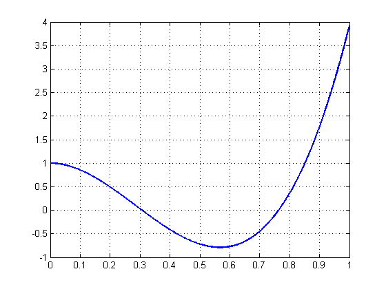
Figure 2: Graph of the function $\varphi=\varphi(h),h\geq 0$ defined by (2.13) with $g=9.8,a_{0}=1,h_{0}=1,u_{0}=1$ and $a=1.2$. The function $\varphi$ admits two zeros in the interval $(0,1)$.

Thus, we arrive at the following lemma.

Lemma 2.2.

Given $U_{0}=(h_{0},u_{0},a_{0})$ and a bottom level $a\neq a_{0}$. The following conclusions holds.

• $a_{\max}(U_{0})\geq a_{0},\quad a_{\max}(U_{0})=a_{0}\quad\textrm{ if and only if}\quad(h_{0},u_{0})\in\mathcal{C}.$

• The nonlinear equation (2.13) admits a root if and only if the condition (2.16) holds, and in this case it has two roots $h_{1}(a)\leq h_{*}\leq h_{2}(a)$. Moreover, whenever the inequality in (2.16) is strict, i.e. $a<a_{\max}(U_{0})$, these two roots are distinct.

• According to the part (ii), whenever (2.16) is fulfilled, there are two states $U_{i}(a)=(h_{i}(a),u_{i}(a),a)$, where $u_{i}(a)=h_{0}u_{0}/h_{i}(a),i=1,2$ to which a stationary contact from $U_{0}$ is possible. Moreover, the locations of these states can be determined as follows

  $$\begin{array}[]{ll}&U_{1}(a)\in G_{1}\quad\textrm{if}\quad u_{0}>0,\\ &U_{1}(a)\in G_{3}\quad\textrm{if}\quad u_{0}<0,\\ &U_{2}(a)\in G_{2}.\\ \end{array}$$

Proof. The parts (i) and (ii) can be easily deduced from the above argument. To prove (iii), it is sufficient to show that along the projection of $\mathcal{W}_{3}(U_{0})$ on the $(h,u)$-plane, the point $U_{\min}(U_{0})=(h_{\min}(U_{0}),u_{\min}(U_{0}):=h_{0}u_{0}/h_{\min}(U_{0}))$, where $h_{\min}(U_{0})$ is defined by (2.15), belongs to $\mathcal{C}_{+}$ if $u_{0}>0$ and belongs to $\mathcal{C}_{-}$ if $u_{0}<0$, and that $U_{i}(a)\in\mathcal{W}_{3}(U_{0}),i=1,2,$ such that $U_{2}(a)\in G_{2}$ and $U_{1}(a)$ is located on the other side of $U_{2}(a)$ with respect to $\mathcal{C}$. Indeed, let us define a function taking values along the stationary curve $\mathcal{W}_{3}(U_{0})$:

$$\sigma(h):=u(h)^{2}-gh={h_{0}^{2}u_{0}^{2}\over h^{2}}-gh.$$

Clearly, a point $U=(h,u,a)$ belongs to $G_{1}\cup G_{3}$ if and only if $\sigma(h)>0$ and $U$ belongs to $G_{2}$ if and only if $\sigma(h)<0$. Since $\sigma(h_{\min}(U_{0}))=0$, the point $U_{\min}(U_{0})$ belongs to $\mathcal{C}$. Obviously, $U_{\min}(U_{0})\in\mathcal{C}_{+}$ if $u_{0}>0$, and $U_{\min}(U_{0})\in\mathcal{C}_{-}$ if $u_{0}<0$. Thus, it remains to check that

$$\sigma(h_{1}(a))>0,\quad\sigma(h_{2}(a))<0.$$ (2.17)

Since

$$\sigma(h_{\min}(U-0))=0,\quad\sigma^{\prime}(h)={-2h_{0}^{2}u_{0}^{2}\over h^{3}}-g<0,$$

we can see that (2.17) holds if

$$h_{1}(a)<h_{\min}(U_{0})<h_{2}(a).$$ (2.18)

On the other hand, we have

$$\begin{array}[]{ll}&\varphi(h)>0,\quad\textrm{if }h<h_{1}(a)\quad\textrm{or}\quad h>h_{2}(a),\\ &\varphi(h)<0,\quad\textrm{if }h_{1}(a)<h<h_{2}(a).\\ \end{array}$$ (2.19)

And we have

$$\varphi(h_{\min}(U_{0}))=3(h_{0}u_{0})^{2}+(2g(a-a_{0}-h_{0})-u_{0}^{2}){(h_{0}u_{0})^{4/3}\over g^{2/3}}.$$

It is a straightforward calculation to show that the condition

$$a<a_{\max}(U_{0})$$

is equivalent to

$$\varphi(h_{\min}(U_{0}))<0.$$

This together with (2.19) establish (2.18). Lemma 2.2 is completely proved. $\scriptstyle\square$

From Lemma 2.2, we can construct two-parameter wave sets. The Riemann problem may therefore admit up to a one-parameter family of solutions. To select a unique solution, we impose an admissibility condition for stationary contacts, referred to as the Monotonicity Criterion and defined as follows:

• Along any stationary curve $\mathcal{W}_{3}(U_{0})$, the bottom level $a$ is monotone as a function of $h$. The total variation of the bottom level component of any Riemann solution must not exceed $|a_{L}-a_{R}|$, where $a_{L},a_{R}$ are left-hand and right-hand bottom levels.

A similar criterion was used [20, 21], [32], and [15].

Lemma 2.3.

The Monotonicity Criterion implies that any stationary shock does not cross the boundary of strict hyperbolicity, in other words:

• If $U_{0}\in G_{1}\cup G_{3}$, then only the stationary contact based on the value $h_{1}(a)$ is allowed, and one sets $\bar{h}(a)=h_{1}(a)$.

• If $U_{0}\in G_{2}$, then only the stationary contact using $h_{2}(a)$ is allowed, and one sets $\bar{h}(a)=h_{2}(a)$.

Thus, $\bar{h}(a)$ is the admissible $h$-value of a right-hand state $U=(h=\bar{h}(a),u,a)$ of the stationary wave from a given left-hand state $U_{0}=(h_{0},u_{0},a_{0})$.

Proof. Recall that the Rankine-Hugoniot relations associate the linearly degenerate field (2.11) implies that the component $a$ can be expressed as a function of $h$:

$$a=a(h)=a_{0}+{-u^{2}+u_{0}^{2}\over 2g}-h+h_{0},$$

where

$$u=u(h)={h_{0}u_{0}\over h}.$$

Thus, taking the derivative of $a$ with respect to $h$, we have

$$\begin{array}[]{ll}a^{\prime}(h)&={-uu^{\prime}(h)\over g}-1=u{h_{0}u_{0}\over gh^{2}}-1\\ &={u^{2}\over gh}-1={(u^{2}-gh)\over gh}\\ \end{array}$$

which has the same sign as $u^{2}-gh$. Thus, $a=a(h)$ is increasing with respect to $h$ in the domains $G_{1},G_{3}$ and is decreasing in the domain $G_{2}$. Thus, in order that $a=a(h)$ is monotone as a function of $h$, the point $(h,u,a)$ must stay in the closure of the domain containing $(h_{0},u_{0},a_{0})$. The conclusions of (i) and (ii) then follow. $\scriptstyle\square$

We now explain how to compute the roots of the equation (2.13). The above argument shows that whenever (2.16) is satisfied, the equation (2.13) admits two roots $h_{1}(a),h_{2}(a)$ satisfying

$$h_{1}(a)\leq h_{\min}=\Big{(}{h_{0}^{2}u_{0}^{2}\over g}\Big{)}^{1/3}\leq h_{*}=\frac{u_{0}^{2}+2g(a_{0}+h_{0}-a)}{3g}\leq h_{2}(a)$$ (2.20)

and the inequalities are all strict whenever the inequality in (2.16) is strict. Since $0<h_{1}(a)\leq h_{\min}\leq h_{*}$ and

$$\begin{array}[]{ll}&\varphi(0)\geq 0,\\ &\varphi(h_{*})\leq 0,\,\varphi(h_{\min})\leq 0,\\ \end{array}$$

the root $h_{1}(a)$ of (2.13) can be computed, for instance using the regula falsi method with the starting interval $[0,h_{\min}]$, or $[0,h_{*}]$. And since $h_{2}(a)\geq h_{*}$ and $\varphi^{\prime}(h)>0,\varphi"(h)>0,h>h_{*}$, the root $h_{2}(a)$ can be computed using Newton’s method with any starting point larger than $h_{*}$. We summarize this in the following lemma.

Proposition 2.4 (Water height of stationary contacts).

The root $h_{1}(a)$ of (2.13) can be computed using the regula falsi method for the starting interval $[0,h_{\min}]$, where $h_{\min}=\Big{(}{h_{0}^{2}u_{0}^{2}\over g}\Big{)}^{1/3}$, or $[0,h_{*}]$, where $h_{*}=\frac{u_{0}^{2}+2g(a_{0}+h_{0}-a)}{3g}$, while the root $h_{2}(a)$ can be computed using Newton’s method with any starting point larger than $h_{*}$.

To conclude this section, we point out that certain physical applications may actually require a different jump relation for the nonconservative product —especially allowing for energy dissipation. This issue will not be addressed further in the present paper, however.

3 The Riemann problem revisited

From the general theory of nonconservative systems of balance laws, it is known that if Riemann data belongs to a sufficiently small ball in a strictly hyperbolic region, then the Riemann problem admits a unique solution. It is worth to note that this result no longer holds if any of these assumptions fails, for instance due to resonance.

Our goal in this section to to provide all possible explicit constructions for Riemann solutions, investigating when data are around the strictly hyperbolic boundary $\mathcal{C}_{\pm}$. There are several improvements in the construction of Riemann solutions in this paper over the ones in our previous work [33]. First, we can determine larger domains of existence by combining constructions in [33] together. Second, the domains where there is a unique solution or there are several solutions are precisely determined. Under the transformation $x\mapsto-x,u\mapsto-u$, a left-hand state $U=(h,u,a)$ in $G_{2}$ or $G_{3}$ will be transferred to the right-hand state $V=(h,-u,a)$ in $G_{2}$ or $G_{1}$, respectively. Thus, the construction for Riemann data around $\mathcal{C}_{-}$ can be obtained from the one for Riemann data around $\mathcal{C}_{+}$. We thus construct only the case where Riemann data are in $G_{1}\cup\mathcal{C}_{+}\cup G_{2}$ and we separate into two regimes on which a corresponding construction based on the left-hand state $U_{L}$ is given:

• Regime (A): $U_{L}\in G_{1}\cup\mathcal{C}_{+}$;

• Regime (B): $U_{L}\in G_{2}$;

For each construction, depending on the location of the right-hand states $U_{R}$ and the sign $a_{R}-a_{L}$ there will be different types of solutions or the results on the existence and uniqueness.

As in [33], to solve (1.1)–(1.3) we project all the wave curves on the $(h,u)$-plane.

Notations

• $U^{0}$ denotes the state resulted from a stationary contact wave from $U$;

• $U^{\#}$ is the state defined in Lemma 2.1 so that $\bar{\lambda}_{1}(U,U^{\#})=0$;

• $W_{k}(U_{i},U_{j})$ ($S_{k}(U_{i},U_{j}),R_{k}(U_{i},U_{j})$) denotes the $k$th-wave ($k$th-shock, $k$th-rarefaction wave, respectively) connecting the left-hand state $U_{i}$ to the right-hand state $U_{j}$, $k=1,2,3$;

• $W_{m}(U_{i},U_{j})\oplus W_{n}(U_{j},U_{k})$ indicates that there is an $m$th-wave from the left-hand state $U_{i}$ to the right-hand state $U_{j}$, followed by an $n$th-wave from the left-hand state $U_{j}$ to the right-hand state $U_{k}$, $m,n\in\{1,2,3\}$.

3.1 Regime (A). Eigenvalues at $U_{L}$ with coinciding signs

Let $\bar{G}_{1}$ denote the closure of $G_{1}$. We assume that $U_{L}\in\bar{G}_{1}$, or equivalently $\lambda_{i}(U_{L})\geq 0,i=1,2,3$.

Construction (A1). In this case (the projection on $(h,u)$-plane of) $U_{R}$ is located in a ”higher” region containing $U_{L}$ in the $(h,u)$-plane.

If $a_{L}\geq a_{R}$ (or $a_{L}<a_{R}\leq a_{\max}(U_{L})$), the solution begins with a stationary contact upward (downward, respectively) along $\mathcal{W}_{3}(U_{L})$ from $U_{L}$ to the state $U_{L}^{o}\in\mathcal{W}_{3}(U_{L})\cap G_{1}$, shifting the level $a_{L}$ directly to the level $a_{R}$. Let

$$\{U_{M}=(h_{M},u_{M},a_{R})\}=\mathcal{W}_{1}(U_{L}^{o})\cap\mathcal{W}_{2}^{B}(U_{R}).$$

Providing that $\bar{\lambda}_{1}(U_{L}^{o},U_{M})\geq 0$, or equivalently, as seen from Lemma 2.1, $h_{M}\leq h_{L}^{o\#}$, the solution can continue by a $1$-wave from $U_{L}^{o}$ to $U_{M}$, followed by a $2$-wave from $U_{M}$ to $U_{R}$. Thus, the solution is

$$W_{3}(U_{L},U_{L}^{o})\oplus W_{1}(U_{L}^{o},U_{M})\oplus W_{2}(U_{M},U_{R}).$$ (3.1)

See Figure 3. This construction can be extended if $\mathcal{W}_{2}^{B}(U_{R})$ lies entirely above $\mathcal{W}_{1}(U_{L}^{o})$. In this case let $I$ and $J$ be the intersection points of $\mathcal{W}_{1}(U_{L}^{o})$ and $\mathcal{W}_{2}^{B}(U_{R})$ with the axis $\{h=0\}$, respectively:

$$\{I\}=\mathcal{W}_{1}(U_{L}^{o})\cap\{h=0\},\quad\{J\}=\mathcal{W}_{2}^{B}(U_{R})\cap\{h=0\},$$ (3.2)

then the solution can be seen as a dry part $W_{o}(I,J)$ between $I$ and $J$. Thus, the solution in this case is

$$W_{3}(U_{L},U_{L}^{o})\oplus R_{1}(U_{L}^{o},I)\oplus W_{o}(I,J)\oplus R_{2}(J,U_{R}).$$

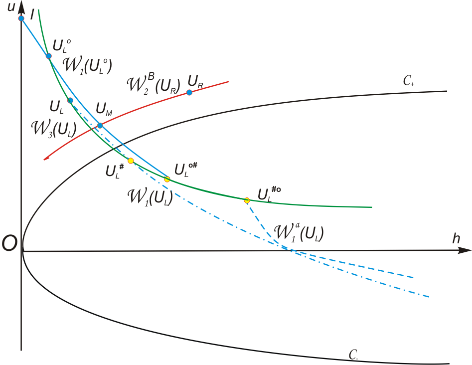
Figure 3: Construction (A1), $a_{L}>a_{R}$: a solution of the form (3.1).

Remark 1.

As seen by Lemma 2.2, if $a_{L}<a_{R}$, the condition

$$a_{R}\leq a_{\max}(U_{L})$$

is necessary for the stationary contact $W_{3}(U_{L},U_{L}^{o})$. Therefore, if this condition fails, there is no solution even if $U_{L}=U_{R}$. The necessary and sufficient conditions for the existence of the solution (3.1) is that $U_{L}^{o\#}$ is located below or on the curve $\mathcal{W}_{2}^{B}(U_{R})$. This domain clearly covers a large crossing-strictly-hyperbolic-boundary neighborhood of $U_{L}$.

Construction (A2). In this construction, we will see an interesting phenomenon when wave speeds associate with different characteristic fields coincide. Roughly speaking, this case concerns with the fact that $U_{R}$ moves limitedly downward from the case $G_{1}$. Instead of using “complete” stationary contact from $U_{L}$ to $U_{L}^{o}$ as in the first possibility, the solution now begins with a “half-way” stationary contact $W_{3}(U_{L},U_{1})$ from $U_{L}=(h,u,a_{L})$ to some state $U_{1}=U_{L}^{o}(a)=(h,u,a)\in\mathcal{W}_{3}(U_{L})$, where $a$ between $a_{L}$ and $a_{R}$. The solution then continues by a $1$-shock wave with zero speed from $U_{1}$ to $U_{2}=U_{1}^{\#}\in\mathcal{W}_{1}(U_{1})\cap G_{2}$. Observe that $U_{2}$ still belongs to $\mathcal{W}_{3}(U_{L})$, since $h_{2}u_{2}=h_{1}u_{1}=h_{L}u_{L}$, as indicated by Lemma 2.1. The solution continues by a stationary contact from $U_{2}$ to a state $U_{M}(a)\in\mathcal{W}_{3}(U_{L})$. The set of these points $U_{M}(a),a\in[a_{L},a_{R}]$ forms a curve pattern denoted by ${\mathcal{L}}$. Whenever

$$\mathcal{W}_{2}^{B}(U_{R})\cap{\mathcal{L}}\neq\emptyset$$

there is a solution containing three discontinuities having the same zero speed of the form

$$W_{3}(U_{L},U_{1})\oplus S_{1}(U_{1},U_{2})\oplus W_{3}(U_{2},U_{M})\oplus W_{2}(U_{M},U_{R}).$$ (3.3)

See Figure 4.

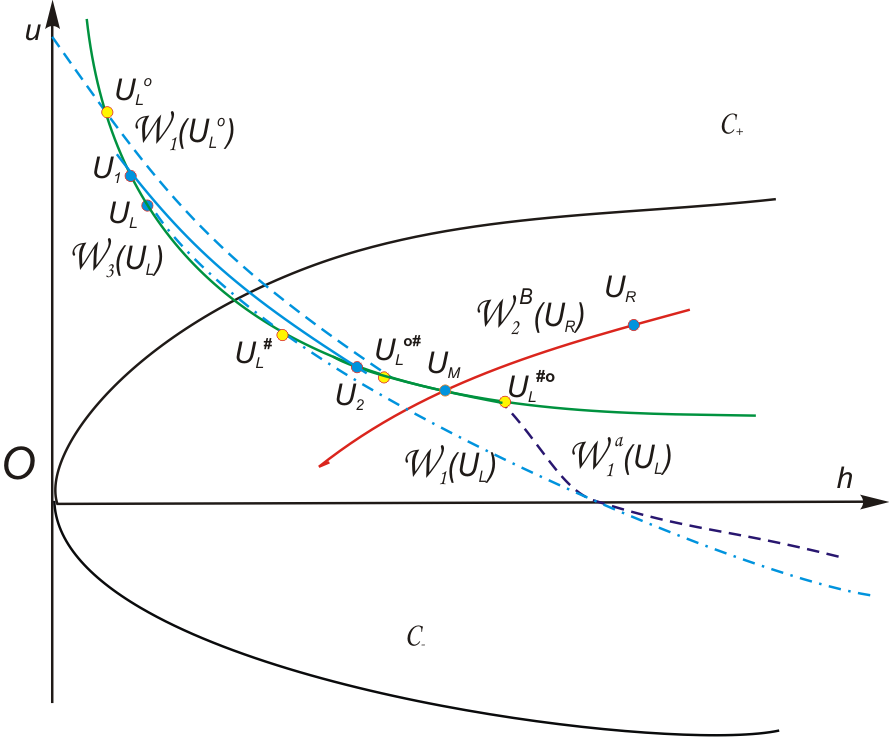
Figure 4: Construction (A2), $a_{L}>a_{R}$: a solution of the form (3.3).

Remark 2.

The necessary and sufficient conditions for the existence of the solution (3.3) is that $U_{L}^{o\#}$ is located above or on the curve $\mathcal{W}_{2}^{B}(U_{R})$, and $U_{L}^{\#o}$ is located below or on the curve $\mathcal{W}_{2}^{B}(U_{R})$. This domain covers a region in $G_{2}^{+}$ and $G_{1}$ which is “far away” from $U_{L}$.

It is interesting that at the limit $a=a_{R}$ at the first jump, we get the first possibility. If $a=a_{L}$, then the solution simply begins with a $1$-shock wave with zero speed followed by a stationary contact shifting $a$ from $a_{L}$ to $a_{R}$. This limit case can be connected to the following possibility.

Construction (A3). The solution begins with a strong $1$-shock wave from $U_{L}$ to any state $U\in\mathcal{W}_{1}(U_{L})\cap G_{2}$ such that $\bar{\lambda}_{1}(U_{L},U)\leq 0$. This shock wave is followed by a stationary contact to a state $U^{o}$ shifting $a$ from $a_{L}$ to $a_{R}$. The set of these states $U^{o}$ form a curve denoted by $\mathcal{W}_{1}^{a}(U_{L})$. That is

$$\begin{array}[]{ll}\mathcal{W}_{1}^{a}(U_{L}):=\{U^{o}:&\exists W_{3}(U,U^{o})\quad\textrm{shifting }a_{L}\quad\textrm{to }a_{R},\\ &U=(h,u,a_{L})\in\mathcal{W}_{1}(U_{L}),\lambda_{1}(U)\leq 0\}.\\ \end{array}$$ (3.4)

Whenever

$$\emptyset\neq\mathcal{W}_{2}^{B}(U_{R})\cap\mathcal{W}_{1}^{a}(U_{L})=\{U_{M}^{o}\}\subset G_{2},\quad\textrm{and}\quad\bar{\lambda}_{2}(U_{M}^{o},U_{R})\geq 0,$$ (3.5)

there will be a Riemann solution defined by

$$S_{1}(U_{L},U_{M})\oplus W_{3}(U_{M},U_{M}^{o})\oplus W_{2}(U_{M}^{o},U_{R}).$$ (3.6)

See Figure 5. In the limit case of (3.3) where $U_{1}\equiv U_{L}$, the solution (3.3) coincides with the solution (3.6).

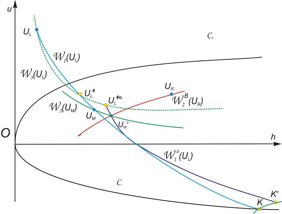
Figure 5: Construction (A3), $a_{L}>a_{R}$: a solution of the form (3.6).

Let $K$ denote the lower limit state on $\mathcal{W}_{1}(U_{L})$ that the solution (3.6) makes sense, and let $K^{o}\in G_{2}$ denote the right-hand state resulted from a stationary contact from $K$ shifting $a_{L}$ to $a_{R}$. Thus, we have

$$\begin{array}[]{ll}&\{K\}=\mathcal{W}_{1}(U_{L})\cap\mathcal{C}_{-},\quad\textrm{if }a_{L}\geq a_{R},\\ &K\in\mathcal{W}_{1}(U_{L})\quad\textrm{such that }a_{\max}(K)=a_{R},\quad\textrm{if }a_{L}<a_{R}.\\ \end{array}$$ (3.7)

Remark 3.

The solution (3.6) makes sense if $U_{L}^{\#o}$ is above or on the curve $\mathcal{W}_{2}^{B}(U_{R})$, and $K^{o}$ lies below or on the curve $\mathcal{W}_{2}^{B}(U_{R})$ and $\bar{\lambda}_{3}(K^{o},U_{R})\geq 0$.

The union of the wave patterns $\mathcal{W}_{1}(U_{1})\cup{\mathcal{L}}\cup\mathcal{W}_{1}^{a}(U_{L})$ form a continuous curve. The Riemann problem thus admits a solution whenever $\mathcal{W}_{2}^{B}(U_{R})$ intersects $\mathcal{W}_{1}(U_{1})\cup{\mathcal{L}}\cup\mathcal{W}_{1}^{a}(U_{L})$ or $\mathcal{W}_{2}^{B}(U_{R})$ intersects with $\{h=0\}$ at a point above the point $I$. We can see that this happens for a large domain of $U_{R}$ containing $U_{L}$. See Figures 3, 4, and 5.

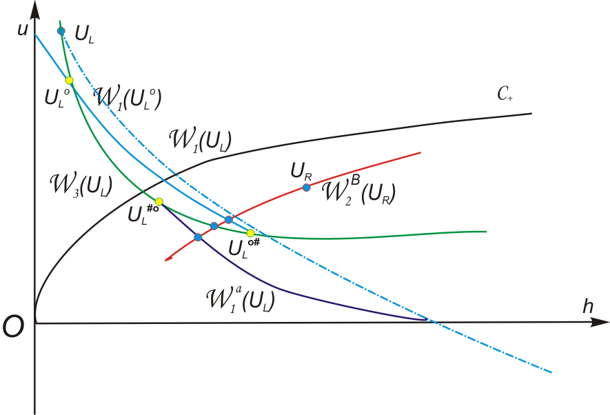
Figure 6: Non-uniqueness: three admissible Riemann solutions of the form (3.1), (3.3), and (3.6).

If the wave pattern ${\mathcal{L}}$ lies entirely on one side with respect to the curve $\mathcal{W}_{2}^{B}(U_{R})$, then $\mathcal{W}_{2}^{B}(U_{R})$ intersects either $\mathcal{W}_{1}(U_{1})$ or $\mathcal{W}_{1}^{a}(U_{L})$ at most one point. Therefore, then (3.1) or (3.6) is the unique solution. Besides, if $\mathcal{W}_{2}^{B}(U_{R})$ intersects the wave pattern ${\mathcal{L}}$, and if $h_{L}^{\#o}\geq h_{L}^{o\#}$, then the point $U_{L}^{\#o}$ is located below the point $U_{L}^{o\#}$ on the curve $\mathcal{W}_{3}(U_{L})$. Thus, the curve $\mathcal{W}_{2}^{B}(U_{R})$ does not meet $\mathcal{W}_{1}(U_{1})$ nor $\mathcal{W}_{1}^{a}(U_{L})$, except possibly at the endpoints $U_{L}^{\#o}\in{\mathcal{L}}$ and $U_{L}^{o\#}\in{\mathcal{L}}$. In this case, (3.3) is the sole solution. In summary, the Riemann problem for (1.1)–(1.2) always has at most one solution whenever $h_{L}^{\#o}\geq h_{L}^{o\#}$.

In the case where $h_{L}^{\#o}<h_{L}^{o\#}$, there can be three solutions, as $\mathcal{W}_{2}^{B}(U_{R})$ can meet all the three curve patterns $\mathcal{W}_{1}(U_{1}),{\mathcal{L}}$ and $\mathcal{W}_{1}^{a}(U_{L})$, or

$$h_{L}^{\#o}<h_{L}^{o\#},\quad\Phi_{2}(U_{L}^{\#o};U_{R})>0>\Phi_{2}(U_{L}^{o\#};U_{R}),$$ (3.8)

where the function $\Phi_{2}(U;U_{R})$ is defined by (2.10). See Figure 6.

The above argument leads us to the following theorem.

Theorem 3.1 (Riemann problem for the shallow water equations).

Given a left-hand state $U_{L}\in G_{1}$. Depending on the location of the right-hand state $U_{R}$ we have the following conclusions.

• Existence. The Riemann problem (1.1)–(1.3) admits a solution if $Q^{o}$ defined in Construction (A3) lies below or on the curve $\mathcal{W}_{2}^{B}(U_{R})$, and that if $\mathcal{W}_{2}^{B}(U_{R})$ intersects with $\mathcal{W}_{1}^{a}(U_{L})$ at some point $U_{M}^{o}\in G_{2}^{-}$, then $\bar{\lambda}_{2}(U_{M}^{o},U_{R})\geq 0$.

• Regime of uniqueness. The Riemann problem (1.1)–(1.3) has at most one solution if

  – either $h_{L}^{\#o}\geq h_{L}^{o\#}$;

  – or $h_{L}^{\#o}<h_{L}^{o\#}$, and the states $U_{L}^{\#o}$ and $U_{L}^{o\#}$ are located on the same side with respect to the curve $\mathcal{W}_{2}^{B}(U_{R})$.

• Multiple solutions. If $h_{L}^{\#o}<h_{L}^{o\#}$, and if the state $U_{L}^{\#o}$ lies above the curve $\mathcal{W}_{2}^{B}(U_{R})$ while the state $U_{L}^{o\#}$ lies below the curve $\mathcal{W}_{2}^{B}(U_{R})$, then the Riemann problem (1.1)–(1.3) has three solutions.

Example. We provide some numerical experiments to illustrate two situations: $h_{L}^{\#o}>h_{L}^{o\#}$, and $h_{L}^{\#o}<h_{L}^{o\#}$ corresponding to the two cases $a_{L}>a_{R}$ (see Tables A1-A3) and $a_{L}<a_{R}$ (see Tables A4, A5). We take at random the state $U_{L}$ and $a_{R}$.

(a) $a_{L}>a_{R}$: all experiments show that $h_{L}^{\#o}>h_{L}^{o\#}$. In Table A1, $U_{L}\in G_{1}$.

Table A1

States $$U_{L}$$

Water Height 0.5 1.1930011 1.1171275

Velocity 4 1.6764444 1.790306

Bottom Level 1 0.9 0.9

In Table A2, $U_{L}\in\mathcal{C}_{+}$.

Table A2

States $$U_{L}$$

Water Height 1 1.3075478 1.2558035

Velocity 3.1304952 2.3941726 2.4928225

Bottom Level 1 0.9 0.9

In Table A3, $U_{L}\in G_{1}$ is far away from $\mathcal{C}_{+}$.

Table A3

States $$U_{L}$$

Water Height 0.01 0.54763636 0.44902891

Velocity 10 0.18260292 0.22270281

Bottom Level 1 0.9 0.9

(b) $a_{L}<a_{R}$: all experiments show that $h_{L}^{\#o}<h_{L}^{o\#}$. In Table A4, $U_{L}\in G_{1}$.

Table A4

States $$U_{L}$$

Water Height 0.5 0.86127059 0.96534766

Velocity 4 2.3221506 2.0717925

Bottom Level 0.9 1 1

In Table A5, $U_{L}\in G_{1}$ is far away from $\mathcal{C}_{+}$.

Table A5

States $$U_{L}$$

Water Height 0.01 1.2748668 1.3718425

Velocity 10 0.78439566 0.72894668

Bottom Level 0.9 1 1

Remark 4.

We conjecture that if $a_{L}>a_{R}$, then $h_{L}^{\#o}>h_{L}^{o\#}$, and if $a_{L}<a_{R}$, then $h_{L}^{\#o}<h_{L}^{o\#}$. If this conjecture holds, then Theorem 3.1 implies that when $a_{L}\geq a_{R}$, the Riemann problem has at most one solution for $U_{L}\in G_{1}$.

3.2 Regime (B). Eigenvalues at $U_{L}$ with opposite signs

In this subsection we consider the case where the left-hand state $U_{L}$ moves downward from the Regime (A): $U_{L}\in\bar{G}_{2}$, or $\lambda_{1}(U_{L})<0=\lambda_{3}(U_{L})<\lambda_{2}(U_{L})$.

Construction (B1). For $U_{R}$ in a “higher” position, there can be two types of solutions depending on whether $a_{L}\geq a_{R}$.

If $a_{L}>a_{R}$ a solution can be constructed as follows. The solution begins from $U_{L}$ with a 1-rarefaction wave until it reaches $\mathcal{C}_{+}$ at a state $U_{1}\in\mathcal{W}_{1}(U_{L})\cap\mathcal{C}_{+}$. A straightforward calculation gives

$$U_{1}=\Big{(}\big{(}{u_{L}\over 3\sqrt{g}}+{2\over 3}\sqrt{h_{L}}\big{)}^{2},{1\over 3}u_{L}+{2\over 3}\sqrt{gh_{L}},a_{L}\Big{)}.$$

This rarefaction wave can be followed by a stationary jump $W_{3}(U_{1},U_{2})$ into $G_{1}$. This stationary wave is possible since $a_{L}\geq a_{R}$. Let $\{U_{3}\}=\mathcal{W}_{1}(U_{2})\cap\mathcal{W}_{2}^{B}(U_{R})$. The solution is then continued by a 1-wave from $U_{2}$ to $U_{3}$, followed by a 2-wave from $U_{3}$ to $U_{R}$. Thus, the solution is given by the formula

$$R_{1}(U_{L},U_{1})\oplus W_{3}(U_{1},U_{2})\oplus W_{1}(U_{2},U_{3})\oplus W_{2}(U_{3},U_{R}).$$ (3.9)

See Figure 7. The construction makes sense if $\bar{\lambda}_{1}(U_{2},U_{3})\geq 0$, which means $U_{3}$ has to be above $U_{2}^{\#}$ on $\mathcal{W}_{1}(U_{2})$. This construction can also be extended if $\mathcal{W}_{2}^{B}(U_{R})$ lies entirely above $\mathcal{W}_{1}(U_{2})$. In this case let $I$ and $J$ be the intersection points of $\mathcal{W}_{1}(U_{2})$ and $\mathcal{W}_{2}^{B}(U_{R})$ with the axis $\{h=0\}$, respectively:

$$\{I\}=\mathcal{W}_{1}(U_{2})\cap\{h=0\},\quad\{J\}=\mathcal{W}_{2}^{B}(U_{R})\cap\{h=0\}.$$

Then, the solution can be seen as containing a dry part $W_{o}(I,J)$ between $I$ and $J$. Thus, the solution in this case is

$$R_{1}(U_{L},U_{1})\oplus W_{3}(U_{1},U_{2})\oplus W_{1}(U_{2},I)\oplus W_{o}(I,J)\oplus R_{2}(J,U_{R}).$$ (3.10)

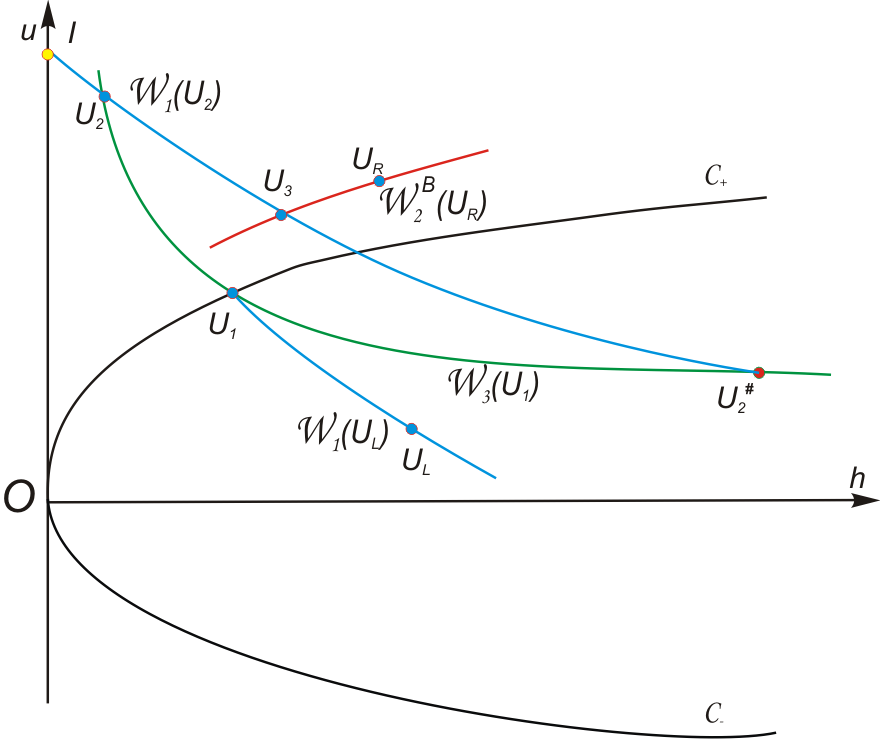
Figure 7: Construction (B1), $a_{L}>a_{R}$: a solution of the form (3.9).

If $a_{L}\leq a_{R}$ a solution of another type can be constructed as follows. To each $U\in\mathcal{C}_{+}$, a stationary contact to $U^{o}\in G_{2}$ downing $a=a_{R}$ to $a=a_{L}$ is possible, since $a_{R}>a_{L}$. The set of all these states $U^{o}$ form a curve denoted by $\mathcal{C}_{+}^{a}$. Let

$$\{U_{1}\}=\mathcal{W}_{1}(U_{L})\cap\mathcal{C}_{+}^{a}.$$

Then, the solution begins by a $1$-wave $W_{1}(U_{L},U_{1})$, followed by a stationary jump $W_{3}(U_{1},U_{2}=U_{1}^{o})$ to $U_{2}\in\mathcal{C}_{+}$. Let $\{U_{3}\}=\mathcal{W}_{1}(U_{2})\cap\mathcal{W}_{2}^{B}(U_{R})$. The solution is then continued by a 1-rarefaction wave from $U_{2}$ to $U_{3}$, followed by a 2-wave from $U_{3}$ to $U_{R}$. Thus, the solution is given by the formula

$$W_{1}(U_{L},U_{1})\oplus W_{3}(U_{1},U_{2})\oplus R_{1}(U_{2},U_{3})\oplus W_{2}(U_{3},U_{R}).$$ (3.11)

See Figure 8. The construction makes sense if $\lambda_{1}(U_{3})\geq 0$, or $U_{3}\in\bar{G}_{1}$. This construction can also be extended if $\mathcal{W}_{2}^{B}(U_{R})$ lies entirely above $\mathcal{W}_{1}(U_{2})$. In this case let $I$ and $J$ be the intersection points of $\mathcal{W}_{1}(U_{2})$ and $\mathcal{W}_{2}^{B}(U_{R})$ with the axis $\{h=0\}$, respectively:

$$\{I\}=\mathcal{W}_{1}(U_{2})\cap\{h=0\},\quad\{J\}=\mathcal{W}_{2}^{B}(U_{R})\cap\{h=0\}.$$

Then, the solution can be seen as containing a dry part $W_{o}(I,J)$ between $I$ and $J$. Thus, the solution in this case is

$$W_{1}(U_{L},U_{1})\oplus W_{3}(U_{1},U_{2})\oplus R_{1}(U_{2},I)\oplus W_{o}(I,J)\oplus R_{2}(J,U_{R}).$$ (3.12)

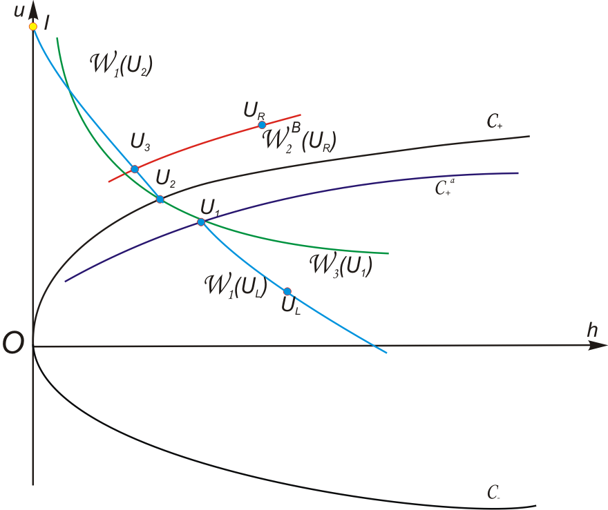
Figure 8: Construction (B1), $a_{L}\leq a_{R}$: a solution of the form (3.11).

The wave structure of the solutions (3.9) and (3.11) are the same, but the state at which the solution reaches the strictly hyperbolic boundary $\mathcal{C}$ using a different wave. However, one may argue that in both cases the solution uses a stationary contact to reach $\mathcal{C}_{+}$ from either side of $\mathcal{C}_{+}$. Moreover, all the states in the solution $(U_{L},U_{1},U_{2},U_{3},U_{R})$ can be in an arbitrarily small ball center on $\mathcal{C}_{+}$.

Construction (B2). This case holds only when $a_{L}>a_{R}$. Again, there is an interesting phenomenon as wave speeds associate with different characteristic fields coincide and all equal zero. The solution therefore contain three waves with the same zero speed.

The solution begins with a $1$-rarefaction wave until it reached $\mathcal{C}_{+}$ at $U_{1}$. At $U_{1}$, the solution may jump to $G_{1}$ using a “half-way” stationary wave to a state $M=M(a)=U_{1}^{o}(a)$ from the bottom height $a_{L}$ to any $a\in[a_{R},a_{L}]$. Then, the solution can continue by a $1$-shock with zero speed from $M$ to $N=N(a)=N^{\#}(a)\in G_{2}^{+}$, followed by a stationary wave from $N$ to $P=P(a)=N^{o}(a)$ with a shift in $a$-component from $a$ to $a_{R}$. The set of these states $P(a)$ form a curve pattern ${\mathcal{L}}$. So, whenever $\emptyset\neq\mathcal{W}_{2}^{B}(U_{R})\cap{\mathcal{L}}=\{P=P(a)\}$, there is a Riemann solution containing three zero-speed waves of the form

$$R_{1}(U_{L},U_{1})\oplus W_{3}(U_{1},M(a))\oplus S_{1}(M(a),N(a))\oplus W_{3}(N(a),P(a))\oplus W_{2}(P(a),U_{R}).$$ (3.13)

See Figure 9.

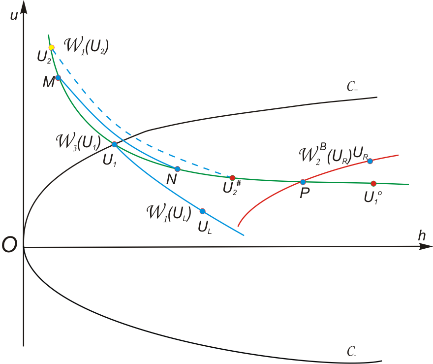
Figure 9: Construction (B2), $a_{L}>a_{R}$: a solution of the form (3.13).

Observe that this solution coincides with the one in Construction (B1) if the first stationary wave from $U_{1}$ to $M=U_{2}$ shifts $a$-component from $a_{L}$ directly to $a_{R}$. The other limit case where the first stationary wave to $G_{1}$ is not used gives a connection to the following possibility.

Construction (B3). In this case the Riemann data can be altogether in a arbitrarily small ball in $G_{2}$. Assume first that $a_{L}\geq a_{R}$. Let

$$\begin{array}[]{ll}&U_{1}=\mathcal{W}_{1}(U_{L})\cap\mathcal{C}_{+},\quad\textrm{and}\quad U_{1}^{0}\in G_{2}+\quad\textrm{ resulted by }\quad W_{3}(U_{1},U_{1}^{o}),\\ &K=\mathcal{W}_{1}(U_{L})\cap\mathcal{C}_{-},\quad\textrm{and}\quad K^{0}\in G_{2}-\quad\textrm{ resulted by}\quad W_{3}(K,K^{o}).\\ \end{array}$$ (3.14)

From any state $U\in\mathcal{W}_{1}(U_{L})$, where $\lambda_{1}(U_{L})\leq 0$ ($U_{L}$ is below $U_{1}$ or coincides with $U_{1}$), we use a stationary jump to a state $U^{o}$, shifting the bottom height from $a_{L}$ down to $a_{R}$. The set of these states $U^{o}$ form a “composite” curve $\mathcal{W}_{1}^{a}(U_{L})$ as defined by (3.4). The curve $\mathcal{W}_{1}^{a}(U_{L})$ is thus a path between $U_{1}^{o}$ and $K^{o}$. Whenever $\emptyset\neq\mathcal{W}_{2}^{B}(U_{R})\cap\mathcal{W}_{1}^{a}(U_{L})=\{U_{M}^{o}\}$, a Riemann solution can be determined by

$$W_{1}(U_{L},U_{M})\oplus W_{3}(U_{M},U_{M}^{o})\oplus W_{2}(U_{M}^{o},U_{R}),$$ (3.15)

where $U_{M}\in\mathcal{W}_{1}(U_{L})$, provided $U_{R}\in G_{2}$ or $\bar{\lambda}_{2}(U_{M}^{o},U_{R})\geq 0$. See Figure 10.

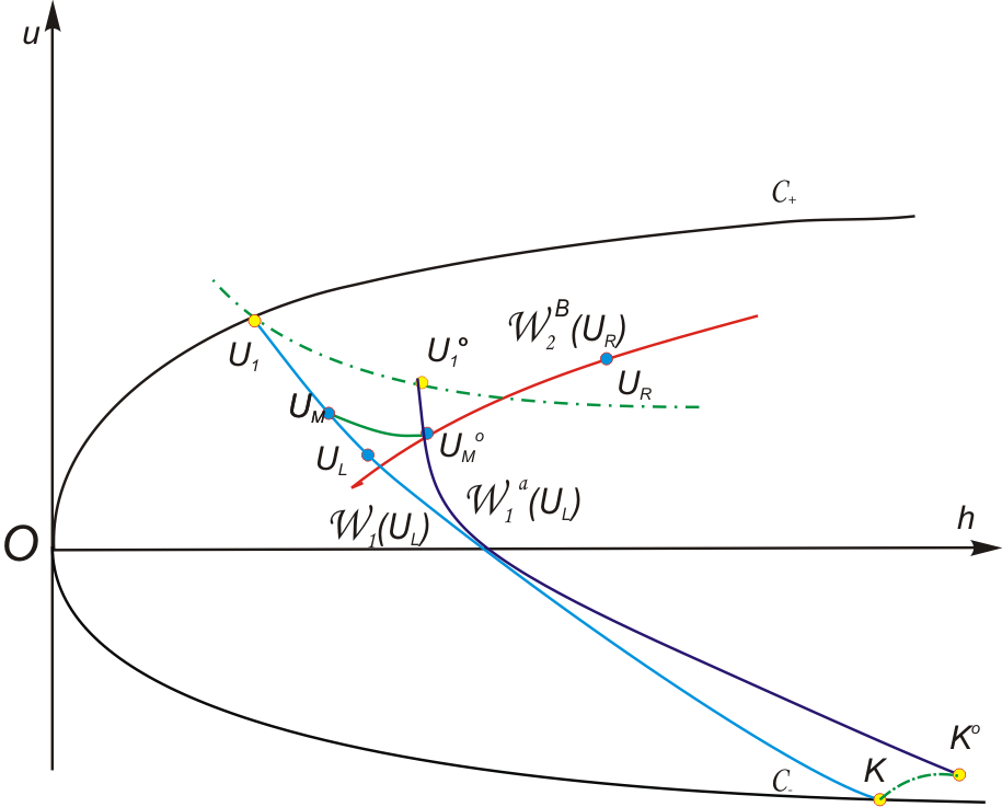
Figure 10: Construction (B3), $a_{L}>a_{R}$: a solution of the form (3.15).

Second, consider the case $a_{L}<a_{R}$. Let $\mathcal{C}_{+}^{a}$ as in the case for the solution of the type (3.15). To each $U\in\mathcal{C}_{\pm}$, a stationary contact to $U^{o}\in G_{2}$ downing back $a=a_{R}$ to $a=a_{L}$ is possible, since $a_{R}>a_{L}$. The set of all these states $U^{o}$ form two curves denoted by $\mathcal{C}_{\pm}^{a}$. Let

$$\begin{array}[]{ll}&\{U_{1}\}=\mathcal{W}_{1}(U_{L})\cap\mathcal{C}_{+}^{a},\quad\textrm{and}\quad U_{1}^{0}\in\mathcal{C}_{+}\quad\textrm{resulted by}\quad W_{3}(U_{1}^{o},U_{1}),\\ &K\in\mathcal{W}_{1}(U_{L}),\quad\textrm{and}\quad K^{0}\in\mathcal{C}_{-}\quad\textrm{resulted by}\quad W_{3}(K^{o},K)\end{array}$$ (3.16)

decreasing $a_{R}$ to $a_{L}$. From any state $U\in\mathcal{W}_{1}(U_{L}),\lambda_{1}(U)\leq\lambda_{1}(U_{1})$, there is a stationary jump to a state $U^{o}$, shifting the bottom height from $a_{L}$ to $a_{R}$. The set of these states $U^{o}$ form a composite curve also denoted by $\mathcal{W}_{1}^{a}(U_{L})$. Whenever $\emptyset\neq\mathcal{W}_{2}^{B}(U_{R})\cap\mathcal{W}_{1}^{a}(U_{L})=\{U_{M}^{o}\}$, a Riemann solution can be determined by

$$W_{1}(U_{L},U_{M})\oplus W_{3}(U_{M},U_{M}^{o})\oplus W_{2}(U_{M}^{o},U_{R}),$$ (3.17)

where $U_{M}\in\mathcal{W}_{1}(U_{L})$, provided $U_{R}\in G_{2}$ or $\bar{\lambda}_{2}(U_{M}^{o},U_{R})\geq 0$.

Remark 5.

In both cases $a_{L}>a_{R}$ and $a_{L}\leq a_{R}$, the condition for $\mathcal{W}_{2}^{B}(U_{R})\cap\mathcal{W}_{1}^{a}(U_{L})\neq\emptyset$ is that $U_{1}^{0}$ lies above $\mathcal{W}_{2}^{B}(U_{R})$ and $K^{o}$ lies below $\mathcal{W}_{2}^{B}(U_{R})$. See Figure 11.

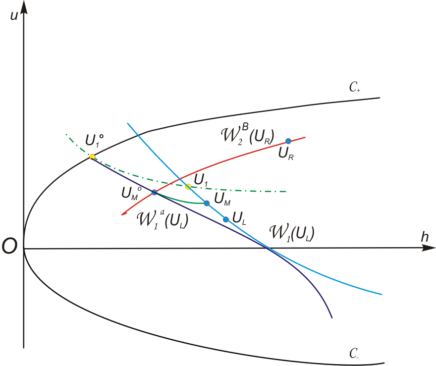
Figure 11: Construction (B3), $a_{L}<a_{R}$: a solution of the form (3.17).

Let us now discuss the existence and uniqueness. Assume first that $a_{L}\leq a_{R}$. In this case, only Constructions (B1) and (B3) are available. The limit case of (3.9) of (B1) when $U_{3}\equiv U_{2}$ coincides with the limit case of (3.15) of (B3). Thus, the union $\mathcal{W}_{1}(U_{2})\cup\mathcal{W}_{1}^{a}(U_{L})$ form a continuous decreasing curve (the curve can be considered as the graph of $u$ being a decreasing function of $h$) and that $\mathcal{W}_{1}(U_{2})$ and $\mathcal{W}_{1}^{a}(U_{L})$ meets only at one point $U_{2}$. Since $\mathcal{W}_{2}^{B}(U_{R})$ is an increasing curve, there always a unique intersection point of $\mathcal{W}_{2}^{B}(U_{R})$ and the union $\mathcal{W}_{1}(U_{2})\cup\mathcal{W}_{1}^{a}(U_{L})$ if $K^{o}$ lies below or on the curve $\mathcal{W}_{2}^{B}(U_{R})$. This implies that the Riemann problem for (1.1)–(1.2) always admits a unique solution if $K^{o}$ lies below or on the curve $\mathcal{W}_{2}^{B}(U_{R})$.

Next, assume that $a_{L}>a_{R}$. Let $U_{1}^{o}\in G_{2}$ denote the state resulted from a stationary wave from $U_{1}\in\mathcal{C}_{+}$. Observe that both $U_{1}^{o}$ and $U_{2}^{\#}$ belong to $\mathcal{W}_{3}(U_{1})$. Whenever $U_{1}^{o}$ lies above $U^{\#}$ on $\mathcal{W}_{3}(U_{1})$, there are three distinct solutions. Otherwise, there is at most one solution. See Figure 12.

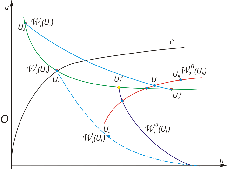
Figure 12: Regime (B): whether $h_{1}^{o}<h_{2}^{\#}$ determines that the Riemann solution is unique or else there exist multiple solutions $U_{L}\in G_{2}$ and $a_{L}>a_{R}$ (cf. Theorem 3.2).

Theorem 3.2 (Riemann problem for the shallow water equations).

Given a left-hand state $U_{L}\in G_{2}$.

• Existence. The Riemann problem (1.1)–(1.3) admits a solution if $K^{o}$ lies below or on the curve $\mathcal{W}_{2}^{B}(U_{R})$, and that if $\mathcal{W}_{2}^{B}(U_{R})$ intersects with $\mathcal{W}_{1}^{a}(U_{L})$ at some point $U_{M}^{o}\in G_{2}^{-}$, then $\bar{\lambda}_{2}(U_{M}^{o},U_{R})\geq 0$.

• Regime of uniqueness. The Riemann problem (1.1)–(1.3) has at most one solution if

  – either $a_{L}\leq a_{R}$;

  – or $a_{L}>a_{R}$, $h_{1}^{o}\geq h_{2}^{\#}$, where $U_{2}$ is defined in (3.9);

  – or $a_{L}>a_{R}$, $h_{1}^{o}<h_{2}^{\#}$, and the states $U_{1}^{o}$ and $U_{2}^{\#}$ are located on the same side with respect to the curve $\mathcal{W}_{2}^{B}(U_{R})$.

• Multiple solutions. If $a_{L}>a_{R}$, $h_{1}^{o}<h_{2}^{\#}$, and $U_{1}^{o}$ lies above the curve $\mathcal{W}_{2}^{B}(U_{R})$ and $U_{2}^{\#}$ lies below the curve $\mathcal{W}_{2}^{B}(U_{R})$, then the Riemann problem (1.1)–(1.3) has three solutions.

Example. We provide some numerical experiments computing $h_{1}^{o},h_{2}^{\#}$ to illustrate the cases of Theorem 3.2 (see Tables B1, B2, and B3). All experiments give the same result: $h_{1}^{o}>h_{2}^{\#}$.

Table B1

States $$U_{L}$$

Water Height 3 1.819500899801235 1.768961248574716

Velocity 0.5 3.032474262659020 3.119112786658156

Bottom Level 1.1 1.000000000000000 1.000000000000000

Table B2

States $$U_{L}$$

Water Height 3 1.707571536932233 1.656818524474798

Velocity 0.1 2.901359698616083 2.990236508448978

Bottom Level 1.1 1.000000000000000 1.000000000000000

Table B3

States $$U_{L}$$

Water Height 3 3.187878980786353 2.574902018055705

Velocity 1 1.969891931767155 2.438841182952260

Bottom Level 2 1.000000000000000 1.000000000000000

Remark 6.

We conjecture that $h_{1}^{o}>h_{2}^{\#}$. If this conjecture holds, then Theorem 3.2 implies that the Riemann problem always has at most one solution for $U_{L}\in G_{2}$.

3.3 Remark on the continuous dependence of solutions

As seen in the previous subsections, the construction of Riemann solutions is based on a given left-hand state $U_{L}$. The Riemann problem for (1.1)–(1.2) admits up to three solutions for data in certain regions, which implies that the initial-value problem for (1.1)–(1.2) is ill-posed. However, connectivity between the types of Riemann solutions helps to determine the continuous dependence of the set of solutions on Riemann data. Observe that for each construction (A) and (B), the general structure of solutions changes continuously when $U_{R}$ changes and one evolves from one case to another. For example, Construction (A1) changes continuously to (A2), and (A2) itself changes continuously to (A3). Similar remarks hold for the cases (B1), (B2), and (B3), as observed earlier about the continuity of the wave patterns. Thus, the set of solutions “globally” depends continuously on the right-hand side $U_{R}$ for each case $U_{L}\in G_{1}\cup\mathcal{C}_{+}$ and $U_{L}\in G_{2}$. In order to show that the set of solutions depends continuously on Riemann data, we need only to check that when $U_{L}$ moves from $G_{1}$ to $G_{2}$, the change in the structure of solutions is continuous as well. But this fact also holds true, since when $U_{L}$ tends to $\mathcal{C}_{+}$ on each side, the solutions in Constructions (A1) and (B1) approach each other, and the solution of Constructions (A3) and (B3) approach each other as long as the solutions make sense. If $a_{L}\geq a_{R}$, these solutions eventually coincide on $\mathcal{C}_{+}$.

4 A Godunov-type algorithm

4.1 A well-balanced quasi-conservative scheme

Given a uniform time step $\Delta t$, and a spatial mesh size $\Delta x$, setting $x_{i}=i\Delta x,i\in\mathbb{Z}$, and $t^{n}=n\Delta t,n\in{\mathbf{N}}$, we denote $U_{i}^{n}$ to be an approximation of the exact value $U(x_{i},t^{n})$. Set

$$U=\left(\begin{array}[]{c}h\\ hu\\ \end{array}\right),\quad F(U)=\left(\begin{array}[]{c}hu\\ h(u^{2}+g\frac{h}{2})\\ \end{array}\right),\quad S(U)=\left(\begin{array}[]{c}0\\ -gh\\ \end{array}\right)\partial_{x}a.$$

The system (1.1)–(1.2) can be written in the compact form

$$\partial_{t}U+\partial_{x}F(U)=S(U)\partial_{x}a,\quad t>0,x\in{R\!\!\!\!\!I~{}}.$$ (4.1)

Let us be given the initial condition

$$U(x,0)=U_{0}(x),\quad x\in{R\!\!\!\!\!I~{}},$$ (4.2)

Then, the discrete initial values $U_{i}^{0}$ are given by

$$U_{i}^{0}={1\over\Delta x}\int_{x_{i-1/2}}^{x_{i+1/2}}U_{0}(x)dx.$$ (4.3)

Suppose $U^{n}$ is known and $U^{n}$ is constant on each interval $(x_{i-1/2},x_{i+1/2})$ v i $i\in\mathbb{Z}$. On each cell $(x_{i-1},x_{i})$ we determine the exact solution to the Riemann problem for

$$\partial_{t}U(x,t)+\partial_{x}F(U(x,t))=S(U)\partial_{x}a,\quad\textrm{on }{R\!\!\!\!\!I~{}}\times(t^{n},t^{n+1}],$$ (4.4)

subject to the initial condition

$$U(x,t^{n})=\left\{\begin{array}[]{ll}U_{i-1}^{n},&\quad x<x_{i-1/2},\\ U_{i}^{n},&x>x_{i-1/2}.\\ \end{array}\right.$$ (4.5)

Denote this solution by $U(x,t;U_{i-1}^{n},U_{i}^{n})$. Use these solutions of the local Riemann problems we define the function $V$ by

$$V(x,t):=\left\{\begin{array}[]{ll}U(x,t;U_{i-1}^{n},U_{i}^{n}),&\quad x_{i-1/2}<x\leq x_{i},t^{n}\leq t\leq t^{n+1},\\ U(x,t;U_{i}^{n},U_{i+1}^{n}),&\quad x_{i}<x\leq x_{i+1/2},t^{n}\leq t\leq t^{n+1}.\\ \end{array}\right.$$

As for the initial values, we have to ensure that the approximation $U_{i}^{n+1}$ at time $t^{n+1}$ is constant on $(x_{i-1/2},x_{i+1/2})$ for all $i\in\mathbb{Z}$. Therefore, we define the new value $U_{i}^{n+1}$ at the time $t=t^{n+1}$ by

$$U_{i}^{n+1}={1\over\Delta x}\int_{x_{i-1/2}}^{x_{i+1/2}}V(x,t^{n+1})dx.$$ (4.6)

This means $U_{i}^{n+1}$ is the mean value of $V$ on $(x_{i-1/2},x_{i+1/2})$ and thus contains parts of $U(x,t;U_{i-1}^{n},U_{i}^{n})$ and $U(x,t;U_{i}^{n},U_{i+1}^{n})$. To ensure that the solutions of two consecutive local Riemann problems do not coincide, we assume that the following CFL (Courant, Friedrichs, Lewy) condition holds:

$${\Delta t\over\Delta x}\max|\lambda_{i}|\leq{1\over 2},$$

where $\lambda_{i}$ denote the eigenvalues of $DF(U)$.

Suppose now $V$ is an exact solution on $(x_{i-1/2},x_{i+1/2})$. Since the $a$-component is constant in $(x_{i-1/2},x_{i+1/2})$, the right-hand side of (1.1) vanishes for $V$. Thus, the standard Godunov scheme is in quasi-conservative form:

$$U_{i}^{n+1}=U_{i}^{n}-{\Delta t\over\Delta x}(F(U(x_{i+1/2}-,t^{n+1};U_{i}^{n},U_{i+1}^{n}))-F(U(x_{i-1/2}+,t^{n+1};U_{i-1}^{n},U_{i}^{n}))).$$ (4.7)

One might think that in the scheme (4.7) the source term is incorporated into the local Riemann problem.

The Godunov scheme (4.7) is capable of capturing exactly equilibria. Therefore (4.7) is a well-balanced scheme. In fact, let us be given the initial data $U^{0}$ to be equilibrium states of a stationary wave. Then, on each cell $x_{i-1/2}<x<x_{i+1/2},t^{n}<t\leq t^{n+1}$ the exact Riemann solution is constant. Thus, $U(x_{i+1/2}-,t^{n};U_{i}^{n},U_{i+1}^{n})=U(x_{i-1/2}+,t^{n};U_{i-1}^{n},U_{i}^{n})$ and so $U_{i}^{n+1}=U_{i}^{n}=U^{0}_{i}$ for all $i\in\mathbb{Z}$ and $n\geq 0$. When there are multiple Riemann solutions, any of them can be selected and we still obtain a deterministic scheme, according to Theorem 3.1.

4.2 Numerical Riemann solver

Given any Riemann data $(U_{L},U_{R})$, denote by $U(x,t;U_{L},U_{R})$ the Riemann solution corresponding to the Riemann data $(U_{L},U_{R})$. To build the Godunov scheme (4.7) we will specify the values $U(0\pm,\Delta t;U_{L},U_{R})$ for an arbitrary and fixed number $\Delta t>0$.

Riemann solver (A1). We present a computing strategy for Riemann solutions (3.1) as follows.

• The state $U_{L}^{o}=(h_{L}^{o},u_{L}^{o},a_{R})$: $h_{L}^{o}=\bar{h}(a_{R})=h_{1}(a_{R})$ , where $h_{1}(a_{R})$ is the smaller root of the nonlinear equation (2.13), described by Lemma 2.1, and can be computed using Lemma 2.4. $u_{L}^{o}=u_{L}h_{L}/h_{L}^{o}$.

• The state $U_{M}=(h_{M},u_{M},a_{R})$ is the intersection point of the wave curves $\mathcal{W}_{1}(U_{L}^{o})$ and $\mathcal{W}_{2}^{B}(U_{R})$, see (2.10). Equating the $u$-component for these two curves leads to a strictly increasing and strictly convex function in $h$. Thus, the $h$-component of the intersection point $h_{2}$ can be computed using the Newton’s method.

The Riemann solver (A1) relying on Construction (A1) yields

$$\begin{array}[]{ll}&U(0-,\Delta t;U_{L},U_{R})=U_{L},\\ &U(0+,\Delta t;U_{L},U_{R})=U_{L}^{o}.\\ \end{array}$$ (4.8)

This implies that the Godunov scheme (4.7) using the Riemann solver 1 becomes

$$U_{i}^{n+1}=U_{i}^{n}-{\Delta t\over\Delta x}(F(U_{i}^{n})-F((U_{i-1}^{n})^{o})),$$ (4.9)

where $U^{o}$ defined as in (4.8).

Riemann solver (A2).

The states of the Riemann solution (3.3) can be found as follows.

• The state $U_{M}=(h_{M},u_{M},a_{R})$ is determined by

  $$\{U_{M}\}=\mathcal{W}_{3}(U_{L})\cap\mathcal{W}_{2}^{B}(U_{R}).$$

• The states $U_{1}=(h_{1},u_{1},a_{1}),U_{2}=(h_{2},u_{2},a_{1})$ are determined by using the corresponding “half-way” shifting in $a$ component from the stationary contact from $U_{L}$ to $U_{1}$ and the stationary contact from $U_{2}$ to $U_{M}$, and using the fact that $U_{2}=U_{1}^{\#}$, (see Lemma 2.1):

  $$\begin{array}[]{ll}&a_{1}=a_{L}+{u_{L}^{2}-u_{1}^{2}\over 2g}+h_{L}-h_{1}=a_{M}+{u_{M}^{2}-u_{2}^{2}\over 2g}+h_{M}-h_{2},\\ &u_{1}=\frac{u_{L}h_{L}}{h_{1}},\\ &h_{2}=\frac{-h_{1}+\sqrt{h_{1}^{2}+8h_{1}u_{1}^{2}/g}}{2},\\ &u_{2}=\frac{u_{M}h_{M}}{h_{2}}.\\ \end{array}$$ (4.10)

It is not difficult to check that the system (4.10) can yield a scalar equation for $h_{1}$. The Riemann solver (A2) relying Construction (A2) gives

$$\begin{array}[]{ll}&U(0-,\Delta t;U_{L},U_{R})=U_{L},\\ &U(0+,\Delta t;U_{L},U_{R})=U_{M}=U_{M}(U_{L},U_{R}).\\ \end{array}$$ (4.11)

This implies that the Godunov scheme (4.7) using the Riemann solver 2 becomes

$$U_{i}^{n+1}=U_{i}^{n}-{\Delta t\over\Delta x}(F(U_{i}^{n})-F(U_{M}(U_{i-1}^{n},U_{i}^{n}))),$$ (4.12)

where $U_{M}(U_{i-1}^{n},U_{i}^{n}))$ is defined as in (4.11), i.e.

$$\{U_{M}(U_{i-1}^{n},U_{i}^{n}))\}=\mathcal{W}_{3}(U_{i-1}^{n})\cap\mathcal{W}_{2}^{B}(U_{i}^{n}).$$

Since $U_{M}$ plays a key role in this Riemann solver, we sketch a computing algorithm for $U_{M}$ as follows. First we observe that if $U_{R}$ lies below the curve $\mathcal{W}_{3}(U_{L})$ in the $(h,u)$-plane, then $U_{M}$ is the intersection point of $\mathcal{W}_{3}(U_{L})$ and $\mathcal{S}_{2}^{B}(U_{R})$. Otherwise, $U_{M}$ is the intersection point of $\mathcal{W}_{3}(U_{L})$ and $\mathcal{R}_{2}^{B}(U_{R})$. Thus, we find:

• (Arrival by a $2$-shock) If $h_{R}u_{R}-h_{L}u_{L}<0$ then $h_{M}$ is the root of the equation

  $$G_{1}(h):={h_{L}u_{L}\over h}-\Big{(}u_{R}+(h-h_{R})\sqrt{{g\over 2}\big{(}{1\over h}+{1\over h_{R}}\big{)}}\Big{)}=0.$$ (4.13)

• (Arrival by a $2$-rarefaction wave) Otherwise, $h_{M}$ is the root of the equation

  $$G_{2}(h):={h_{L}u_{L}\over h}-\big{(}u_{R}+2\sqrt{g}(\sqrt{h}-\sqrt{h_{R}})\big{)}=0.$$ (4.14)

It is easy to see that both functions $G_{1},G_{2}$ defined by (4.13) and (4.14) are strictly convex. Moreover, we have

$$\begin{array}[]{ll}G_{1}^{\prime}(h)&=-{h_{L}u_{L}\over h^{2}}-\sqrt{g\over 2}\Big{(}{1\over h}+{2\over h_{R}}+{h_{R}\over h^{2}}\Big{)}\Big{(}\frac{1}{2\sqrt{1/h+1/h_{R}}}\Big{)}<0,\\ G_{2}^{\prime}(h)&=-{h_{L}u_{L}\over h^{2}}-\sqrt{g\over h}<0,\end{array}$$

for all $h>0$. Thus, the Newton method can be applied for both equations (4.13) and (4.14) with any starting point.

Riemann solver (A3).

Let us consider Construction (A3) and let

$$A=U_{L}^{\#},\quad\{B\}=\mathcal{W}_{1}(U_{L})\cap\mathcal{W}_{2}^{B}(U_{R}).$$

It is easy to see that $U_{M}=(h_{M},u_{M},a_{L})$ lies on $\mathcal{W}_{1}(U_{L})$ between $A$ and $B$. We propose a procedure similar to the Bisection method to compute the states of the elementary waves of the Riemann solution (3.6) as follows. We use the equation of $\mathcal{W}_{2}^{B}(U_{R}):\Phi_{2}(U;U_{R})=0$, defined by (2.10), as a test condition: for $U$ above $\mathcal{W}_{2}^{B}(U_{R})$, $\Phi_{2}(U;U_{R})>0$ and for $U$ below it, $\Phi_{2}(U;U_{R})<0$. Using a stationary jump from any state $U$ on the wave pattern of $\mathcal{W}_{1}(U_{L})$ between $A$ and $B$ to a state $U^{o}$ shifting $a$ from $a_{L}$ to $a_{R}$. Then, we have

$$\Phi_{2}(A;U_{R})\cdot\Phi_{2}(B;U_{R})<0.$$

Algorithm 1:

Step 1: An estimate for $h_{M}$ is given by

$$h_{M}={h_{A}+h_{B}\over 2},$$

$U_{M}=(h_{M},u_{M},a_{L})\in\mathcal{W}_{1}(U_{L})$, so $u_{M}$ is computed using the equation (2.6) with $U_{0}=U_{L}$.

Step 2:

• If $\Phi_{2}(A;U_{R})\cdot\Phi_{2}(U_{M};U_{R})<0$, then set $B=U_{M}$ and return to Step 1;

• If $\Phi_{2}(A;U_{R})\cdot\Phi_{2}(U_{M};U_{R})>0$, then set $A=U_{M}$ and return to Step 1;

• If $\Phi_{2}(A;U_{R})\cdot\Phi_{2}(U_{M};U_{R})=0$, terminate the computation.

We can still use an alternative algorithm using the value of $a$-component as a convergence condition, as follows.

Algorithm 2:

Step 1: Let $A=U_{L}^{\#}$ and $B$ is the intersection point of $\mathcal{W}_{1}(U_{L})$ and $\{u=0\}$. An estimate for $h_{M}$ is given by

$$h_{M}={h_{A}+h_{B}\over 2},$$

and $u_{M}$ is estimated using the equation (2.6), so an estimate of $U_{M}$ is $U_{M}=(h_{M},u_{M},a_{L})\in\mathcal{W}_{1}(U_{L})$. An estimate for $U_{M}^{o}$ is given by

$$\{U_{M}^{o}\}=\mathcal{W}_{3}(U_{M})\cap\mathcal{W}_{2}^{B}(U_{R}).$$

Determine the change in $a$-component for the stationary wave between $U_{M}$ and $U_{M}^{o}$ (see (2.12))

$$a=a_{L}+{u_{M}^{2}-(u_{M}^{o})^{2}\over 2g}+h_{M}-h_{M}^{o}.$$

Step 2:

• If $a-a_{R}<0$, then set $h_{A}=h_{M}$ and return to Step 1;

• If $a-a_{R}>0$, then set $h_{B}=h_{M}$ and return to Step 1;

• If $a-a_{R}=0$, stop the computation.

The Riemann solver (A3) relying on Construction (A3) yields

$$\begin{array}[]{ll}&U(0-,\Delta t;U_{L},U_{R})=U_{M}=U_{M}(U_{L},U_{R}),\\ &U(0+,\Delta t;U_{L},U_{R})=U_{M}^{o}=(U_{M}(U_{L},U_{R}))^{o}.\\ \end{array}$$ (4.15)

This implies that the Godunov scheme (4.7) using the Riemann solver 3 becomes

$$U_{i}^{n+1}=U_{i}^{n}-{\Delta t\over\Delta x}(F(U_{M}(U_{i}^{n},U_{i+1}^{n}))-F(U_{M}^{o}(U_{i-1}^{n},U_{i}^{n}))),$$ (4.16)

where $U_{M}(U_{i}^{n},U_{i+1}^{n})$ and $U_{M}^{o}(U_{i-1}^{n},U_{i}^{n}))$ are defined as in (4.15).

Riemann solver (B1). The Riemann solver (B1) relying on Construction (B1) gives

$$\begin{array}[]{ll}&U(0-,\Delta t;U_{L},U_{R})=U_{1}=\Big{(}\big{(}{u_{L}\over 3\sqrt{g}}+{2\over 3}\sqrt{h_{L}}\big{)}^{2},{1\over 3}u_{L}+{2\over 3}\sqrt{gh_{L}},a_{L}\Big{)}:=U_{L,+}\in\mathcal{C}_{+},\\ &U(0+,\Delta t;U_{L},U_{R})=U_{2}:=U_{L,+o}\in G_{1},\\ \end{array}$$ (4.17)

If $a_{L}\geq a_{R}$, then

$$\begin{array}[]{ll}&U_{1}=\Big{(}\big{(}{u_{L}\over 3\sqrt{g}}+{2\over 3}\sqrt{h_{L}}\big{)}^{2},{1\over 3}u_{L}+{2\over 3}\sqrt{gh_{L}},a_{L}\Big{)}:=U_{L,+}\in\mathcal{C}_{+},\\ &U_{2}:=U_{L,+o}\in G_{1},\\ \end{array}$$

where $U_{L,+o}\in G_{1}$ is the state resulted by a stationary contact from $U_{L,+}\in\mathcal{C}_{+}$. This implies that the Godunov scheme (4.7) using the Riemann solver (B1) becomes

$$U_{i}^{n+1}=U_{i}^{n}-{\Delta t\over\Delta x}(F(U_{i,+}^{n})-F(U_{i-1,+o}^{n})).$$ (4.18)

If $a_{L}<a_{R}$, then $U_{2}\in\mathcal{C}_{+}$. The computing of $U_{1}$ and $U_{2}$ can be done similarly as in the Riemann solver (A3).

Riemann solver (B2). The Riemann solver (B2) relying Construction (B2) gives

$$\begin{array}[]{ll}&U(0-,\Delta t;U_{L},U_{R})=U_{1}=\Big{(}\big{(}{u_{L}\over 3\sqrt{g}}+{2\over 3}\sqrt{h_{L}}\big{)}^{2},{1\over 3}u_{L}+{2\over 3}\sqrt{gh_{L}},a_{L}\Big{)}:=U_{L,+}\in\mathcal{C}_{+},\\ &U(0+,\Delta t;U_{L},U_{R})=P=P(U_{L},U_{R})\in\mathcal{W}_{2}^{B}(U_{R})\cap\mathcal{W}_{3}(U_{L,+}).\\ \end{array}$$ (4.19)

This implies that the Godunov scheme (4.7) using the Riemann solver 2 becomes

$$U_{i}^{n+1}=U_{i}^{n}-{\Delta t\over\Delta x}(F(U_{i,+}^{n})-F(P(U_{i-1}^{n},U_{i}^{n}))),$$ (4.20)

where

$$P(U_{i-1}^{n},U_{i}^{n}))=\mathcal{W}_{2}^{B}(U_{i}^{n})\cap\mathcal{W}_{3}(U_{i-1,+}^{n}).$$

Riemann solver (B3). The Riemann solver (B3) relying on Construction (B3) yields

$$\begin{array}[]{ll}&U(0-,\Delta t;U_{L},U_{R})=U_{M}=U_{M}(U_{L},U_{R}),\\ &U(0+,\Delta t;U_{L},U_{R})=U_{M}^{o}=(U_{M}(U_{L},U_{R}))^{o}.\\ \end{array}$$ (4.21)

This implies that the Godunov scheme (4.7) using the Riemann solver 3 becomes

$$U_{i}^{n+1}=U_{i}^{n}-{\Delta t\over\Delta x}(F(U_{M}(U_{i}^{n},U_{i+1}^{n}))-F(U_{M}^{o}(U_{i-1}^{n},U_{i}^{n}))),$$ (4.22)

where $U_{M}(U_{i}^{n},U_{i+1}^{n})$ and $U_{M}^{o}(U_{i-1}^{n},U_{i}^{n}))$ are defined as in (4.21). It is easy to see that the determinations of the states $U(0-,\Delta t;U_{L},U_{R})$ and $U(0+,\Delta t;U_{L},U_{R})$ by Solvers (A3) and (B3) are the same.

The computing strategies for Solvers (B1), (B2), and (B3) are similar to those of Solvers (A1), (A2), and (A3).

4.3 The Godunov algorithm

It is natural to ask which Riemann solvers should be taken in the Godunov scheme. As seen earlier, in the regions where there are possibly multiple solutions one can select any Riemann solution. Three extreme cases can be distinguished by preferring one particular Riemann solver whenever it is available. For example, we can decide to always select solutions with stationary contact wave in the same region as the left-hand state, that is, the solvers (A1) and (B3). This selection leads us to a deterministic algorithm for designing a corresponding Godunov scheme, as now described.

Building Godunov Scheme Algorithm preferring solvers (A1) and (B3). Let $U_{L}=U_{i}^{n}$ and $U_{R}=U_{i+1}^{n}$.

If $\lambda_{1}(U_{L})\leq 0$

If $\Phi_{2}(U_{L}^{o\#};U_{R})<0$

Use Solver (A1)

elseif $\Phi_{2}(U_{L}^{\#o};U_{R})<0$

Use Solver (A2)

else

Use Solver (A3)

end

else

If $\Phi_{2}(U_{1}^{o};U_{R})>0$

Use Solver (B3)

elseif $\Phi_{2}(U_{2}^{\#};U_{R})>0$

Use Solver (B2)

else

Use Solver (B1)

end

end

5 Numerical experiments (I). The non-resonant regime

We now numerically investigate our Riemann solver and Godunov method and present several numerical tests. For each test we consider the errors between the exact Riemann solution and the approximate solution by the Godunov scheme (4.7) for $x\in[-1,1]$ with different mesh sizes corresponding to $500,1000,2000$ points. In this section as well as in the next section, we plot the solution at the time $t=0.1$, and use the stability condition

$$CFL=0.75.$$

The algorithm for selecting the Riemann solvers is the one described at the end of the last section, unless indicated otherwise.

5.1 Test 1

This test indicates that the Godunov method is capable of maintaining equilibrium states. Let

$$U_{0}(x)=\left\{\begin{array}[]{ll}&U_{L}=(h_{L},u_{L},a_{L}),\quad x<0\\ &U_{R}=(h_{R},u_{R},a_{R}),\quad x>0,\\ \end{array}\right.$$ (5.1)

where $U_{L}=(1,5,1)$ and $U_{R}=(1.223655890827479,4.086116070277590,1.2)$. It is not difficult to check that the Riemann problem with initial data (5.1) admits a stationary contact between these equilibrium states:

$$U(x,t)=U_{0}(x),\quad x\in{R\!\!\!\!\!I~{}},t>0.$$ (5.2)

Figure 13 shows that the stationary contact is well captured by Godunov method using our exact Riemann solver for $x\in[-1,1]$ with $500$ mesh points and at time $t=0.1$.

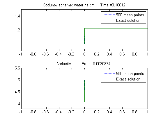
Figure 13: Test 1: A stationary contact wave is captured exactly by Godunov method using our exact Riemann solver.

5.2 Test 2

We now approximate a non-stationary Riemann solution with data $U_{L},U_{R}\in G_{1}$. Precisely, we consider the Riemann problem (1.1)–(1.3) with data

$$U_{0}(x)=\left\{\begin{array}[]{ll}&U_{L}=(h_{L},u_{L},a_{L})=(0.3,2,1.1)\in G_{1},\quad x<0,\\ &U_{R}=(h_{R},u_{R},a_{R})=(0.4,2.2,1)\in G_{1},\quad x>0.\\ \end{array}\right.$$ (5.3)

The Riemann problem (1.1)–(1.2) with the initial data (5.3) admits the solution described by Construction 1, where

$$\begin{array}[]{ll}&U_{1}=(0.21815897,2.750288,1),\qquad\quad U_{2}=(0.35252714,1.9572394,1).\\ \end{array}$$

The errors for Test 2 are reported in the following table

$$N$$

500 0.012644

1000 0.0087928

2000 0.0063773

and Figures 14 and 15 and the table above show that approximate solutions are closer to the exact solution when the mesh size gets smaller.

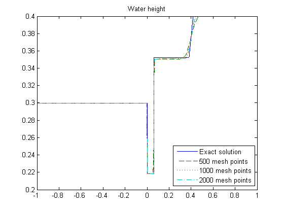
Figure 14: Test 2. Water height with different mesh sizes.

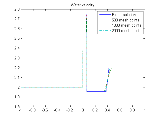
Figure 15: Test 2. Water velocity with different mesh sizes.

5.3 Test 3

In this test, we will approximate a non-stationary Riemann solution with Riemann data $U_{L},U_{R}\in G_{2}$. Precisely, we consider the Riemann problem (1.1)–(1.3) with data

$$U_{0}(x)=\left\{\begin{array}[]{ll}&U_{L}=(h_{L},u_{L},a_{L})=(1,3,1.2)\in G_{2},\quad x<0,\\ &U_{R}=(h_{R},u_{R},a_{R})=(2,0.5,1)\in G_{2},\quad x>0.\\ \end{array}\right.$$ (5.4)

This problem admits the solution described by Construction (A3), where

$$\begin{array}[]{ll}&U_{M}=(1.8452179,0.67672469,1.2),\qquad\quad U_{M}^{o}=(2.0496463,0.60922927,1).\\ \end{array}$$

Precisely, the solution starts with a 1-shock from $U_{L}$ to $U_{M}$, followed by a stationary contact from $U_{M}$ to $U_{M}^{o}$, and then arrived at $U_{R}$ from $U_{M}^{o}$ by a 2-shock wave. The errors for Test 3 are reported in the following table:

$$N$$

500 0.01813

1000 0.0076434

2000 0.0035277

(5.5)

Figures 16 and 17 and the table above show that approximate solutions are closer to the exact solution when the mesh size gets smaller. All of our tests presented so far exhibit a convergence of approximate solutions to the exact solution.

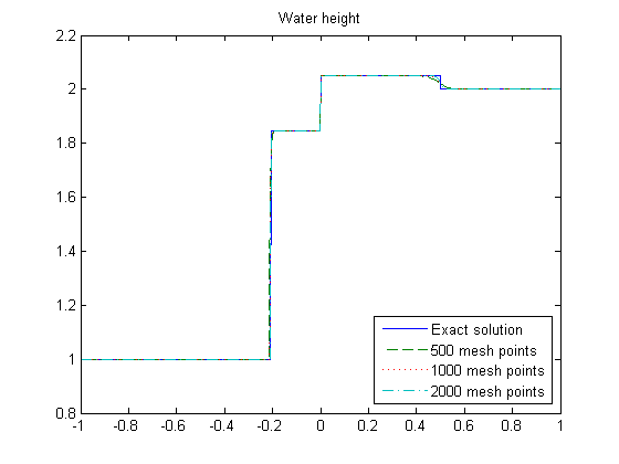
Figure 16: Test 3. Water height with different mesh sizes.

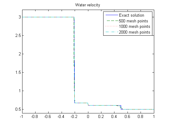
Figure 17: Test 3. Water velocity with different mesh sizes.

6 Numerical experiments (II). The resonance regime

In the following, we will consider the cases where the Riemann data on the different sides with respect to $\mathcal{C}_{+}$:

• $U_{L}\in G_{1}$ and $U_{R}\in G_{2}$;

• $U_{L}\in G_{2}$ and $U_{R}\in G_{1}$.

The solution is evaluated for $x\in[-1,1]$ with $500$ points and at time $t=0.1$. We take also

$$CFL=0.75.$$

6.1 Test 4

In this test, $a_{L}>a_{R}$, and there is a unique solution. We consider the Riemann problem (1.1)–(1.3) with data

$$U_{0}(x)=\left\{\begin{array}[]{ll}&U_{L}=(h_{L},u_{L},a_{L})=(1,3,1.1)\in G_{1},\quad x<0,\\ &U_{R}=(h_{R},u_{R},a_{R})=(1.2,0.1,1)\in G_{2},\quad x>0.\\ \end{array}\right.$$ (6.1)

We have

$$h_{L}^{o\#}=1.042865405801653<h_{L}^{\#o}=1.213385283426733.$$

Thus, the problem (1.1), (1.2), (6.1) admits a unique solution of the form (3.1), according to Theorem (3.1), where

$$U_{M}=(1.5521168,1.4328264,1.1),\quad U_{M}^{o}=(1.665941,1.3349296,1).$$

Figures 18-19 show that the Godunov scheme gives good approximate solutions to the exact solution in this resonance case.

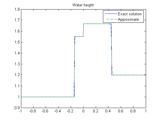
Figure 18: Test 4 (Resonant case). Water height of the solution (3.6).

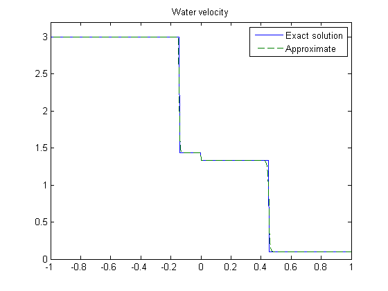
Figure 19: Test 4 (Resonant case). Water velocity of the solution (3.6).

6.2 Test 5

In this test, $a_{L}<a_{R}$, and there is a unique solution. We consider the Riemann problem (1.1)–(1.3) with data

$$U_{0}(x)=\left\{\begin{array}[]{ll}&U_{L}=(h_{L},u_{L},a_{L})=(0.2,4,1)\in G_{1},\quad x<0,\\ &U_{R}=(h_{R},u_{R},a_{R})=(0.5,1.5,1.1)\in G_{2},\quad x>0,\\ \end{array}\right.$$ (6.2)

and

$$\begin{array}[]{ll}&U_{L}^{o\#}=(0.677264819960833,1.181221844722815),\\ &\Phi_{2}(U_{L}^{o\#};U_{R})=-1.050411375011095<0,\\ &U_{L}^{\#o}=(0.581828763814630,1.374974992221044),\\ &\Phi_{2}(U_{L}^{\#o};U_{R})=-0.474326705580410<0.\\ \end{array}$$

This Riemann problem admits a unique solution of the form (3.1), according to Theorem 3.1, where

$$U_{L}^{o}=(0.21591647,3.7051366,1.1),\quad U_{M}=(0.56185289,1.7661913,1.1).$$

Figures 20 to 21 show that the Godunov scheme gives good approximate solutions to the exact solution in this resonance case.

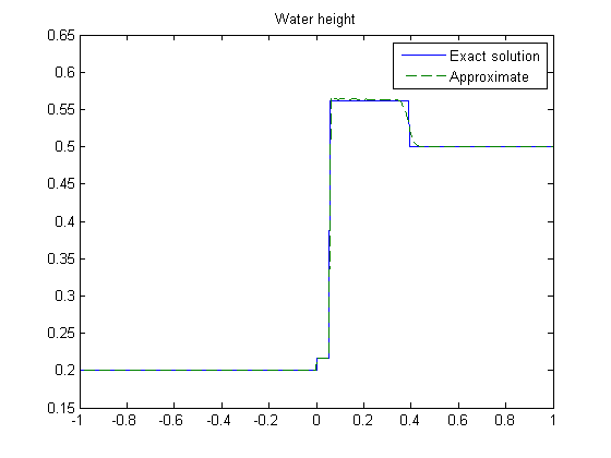
Figure 20: Test 5 (Resonant case). Water height of the solution (3.1).

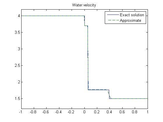
Figure 21: Test 5 (Resonant case). Water velocity of the solution (3.1).

6.3 Test 6

Next, we provide a test for the case there are multiple solutions. So we consider the Riemann problem (1.1)–(1.3) with data

$$U_{0}(x)=\left\{\begin{array}[]{ll}&U_{L}=(h_{L},u_{L},a_{L})=(0.2,5,1)\in G_{1},\quad x<0,\\ &U_{R}=(h_{R},u_{R},a_{R})=(0.75904946,1.3410741,1.2)\in G_{2},\quad x>0.\\ \end{array}\right.$$ (6.3)

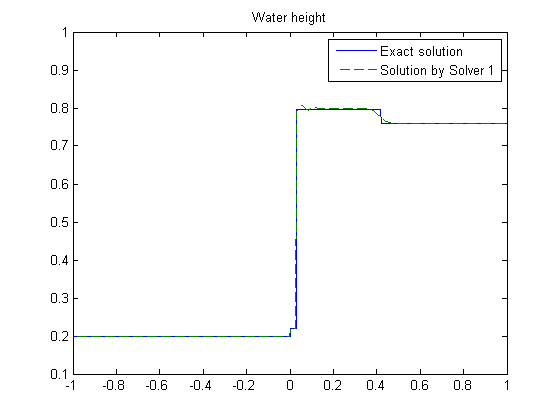
Figure 22: Test 6 (Resonant case - multiple solutions). Water height of the solution (3.1) - preferred Solver (A1).

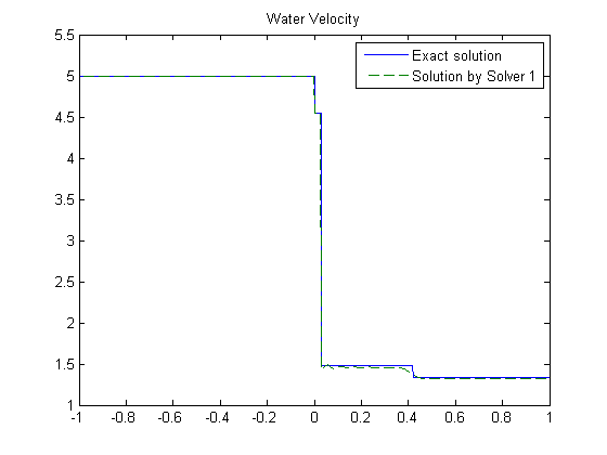
Figure 23: Test 6 (Resonant case - multiple solutions). Water velocity of the solution (3.1) - preferred Solver (A1).

The Riemann problem (1.1)–(1.3) with initial data (6.3) admits three distinct solutions: one solution of the form (3.1) with

$$U_{L}^{o}=(0.21984063,4.5487497,1.2),\quad U_{M}=(0.7964266,1.4737915,1.2),$$ (6.4)

one solution of the form (3.3) with

$$U_{M}=(0.75904946,1.3174372,1.2),$$ (6.5)

which can be seen to be a stationary solution, and one solution of the form (3.6) with

$$U_{M}=(0.95328169,0.89892673,1),\quad U_{M}^{o}=(0.72279573,1.1855776,1.2).$$ (6.6)

We could have three extreme choices of a Riemann solver for the Godunov method in this case. This can be seen easily by saying that we prefer a particular solver whenever it is available. From Figures 22 and 23 it follows that if Solver (A1) is preferred whenever it is available, then the approximate solution approaches the exact solution. The same observation for Solver (A2); see Figures 24 and 25. However, it is not the case for Solver (A3): approximate solutions do not converge to the exact Riemann solution by (3.6); see Figures 26 and 27.

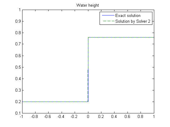
Figure 24: Test 6 (Resonant case - multiple solutions). Water height of the solution (3.3) preferred Solver (A2).

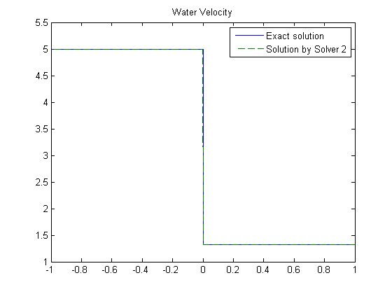
Figure 25: Test 6 (Resonant case - multiple solutions). Water velocity of the solution (3.3) - preferred Solver (A2).

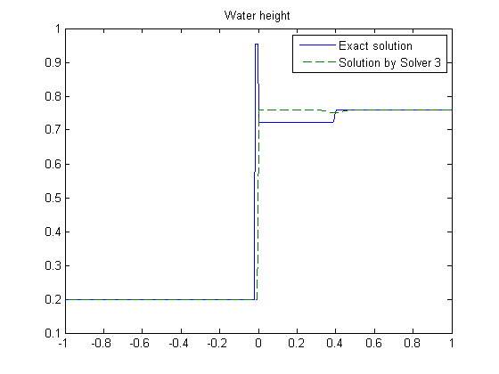
Figure 26: Test (Resonant case - multiple solutions). Water height of the solution (3.6) - preferred Solver (A3).

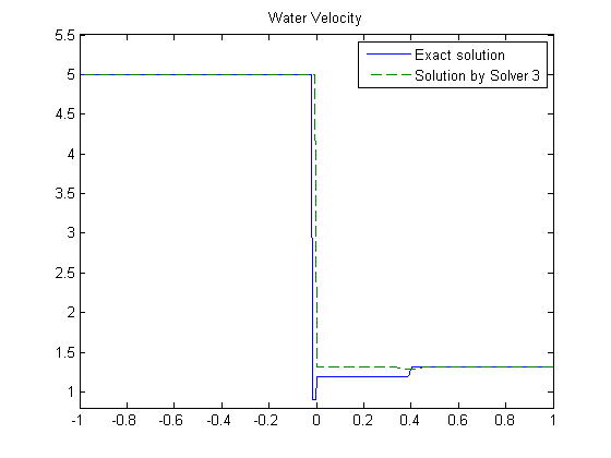
Figure 27: Test 6 (Resonant case - multiple solutions). Water height of the solution (3.6) - preferred Solver (A3).

6.4 Test 7

Finally, we consider the Riemann problem with data

$$U_{0}(x)=\left\{\begin{array}[]{ll}&U_{L}=(h_{L},u_{L},a_{L})=(1,2,1.1)\in G_{2},\quad x<0,\\ &U_{R}=(h_{R},u_{R},a_{R})=(0.8,4,1)\in G_{1},\quad x>0.\\ \end{array}\right.$$ (6.7)

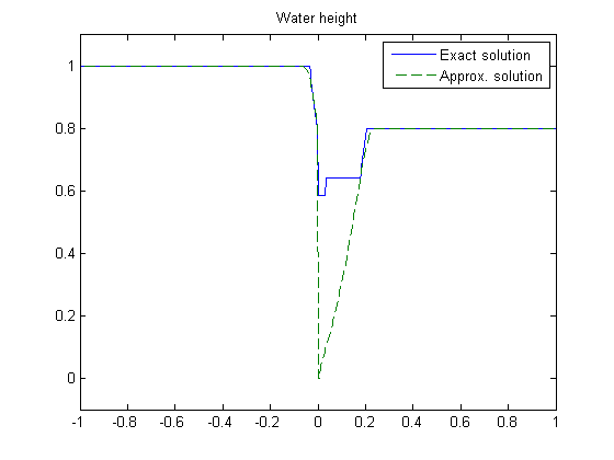
Figure 28: Test 7 (Resonant case). Water height of the solution (3.10). The Godunov scheme does not approach the exact solution in this resonance case.

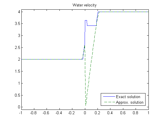
Figure 29: Test 7 (Resonant case. Water velocity for (3.10). The Godunov scheme does not approach the exact solution in this resonance case.

We have

$$h_{2}^{\#}=0.998204556070240<h_{1}^{o}=1.050890579855180,$$

where $h_{2}^{\#},h_{1}^{o}$ are defined as in Theorem (3.2). Thus, the problem (1.1), (1.2), (6.1) admits a unique solution of the form (3.10), according to Theorem (3.2), where

$$\begin{array}[]{ll}&U_{1}=(0.77374106,2.7536634,1.1),U_{2}=(0.58589019,3.636556,1),\\ &U_{3}=(0.64142927,3.4143821,1).\end{array}$$ (6.8)

Precisely, the solution begins with a $1$-rarefaction wave from $U_{L}$ to $U_{1}$, followed by a stationary contact from $U_{1}$ to $U_{2}$, then continued by a 1-shock wave from $U_{2}$ to $U_{3}$, and finally attains $U_{R}$ by a 2-rarefaction from $U_{3}$. Figures 28-29 show that the Godunov scheme generates approximate solutions which do not approach the exact solution in this resonance case (here shown at time $t=0.03$).

7 Concluding remarks

In this paper, we have provided for the first time a complete characterization of all solutions to the Riemann problem associated with the shallow water equations. First, we determined domains in the phase space in which precisely one solution exists and domains in which several solutions (up to three) are available. Second, we provided a computing strategy which allowed us to numerically determine all possible Riemann solutions. Third, we defined a well-balanced and quasi-conservative Godunov scheme, which was carefully tested in several regimes of interest.

The following main conclusions were established in this paper:

• The proposed scheme captures exactly the equilibrium states.

• It converges to the uniquely defined solution to the Riemann problem in strictly hyperbolic domains of the phase space, and this property validates our numerical strategy. We emphasize that the existing literature restricts attention to this strictly hyperbolic regime, only.

• Next, in order to further test our new algorithm, we considered Riemann data belonging to both sides of the resonance curve; both convergence to the selected solution and as well as convergence to another solution were observed. This is not surprising since multiple solutions are available in such a regime.

• Finally, the most challenging test was performed by taking states precisely on the resonance curve, and we observed that the scheme gave quite unsatisfactory results with no convergence whatsoever observed. This latter behavior should not be interpreted as a drawback of the numerical method itself, but rather indicates a limitation of the physical model which, in itself, does not properly describe the fluid flow so that further physics is required in this regime. It is conceivable that a more satisfactory model could be obtained by analyzing the (small-scale) effects of higher-order terms and, for instance, introducing a suitable notion of kinetic relation, similarly to what is done for undercompressive shock waves [28, 29].

References

References

- [1] F. Alcrudo and F. Benkhaldoun, Exact solutions to the Riemann problem of the shallow water equations with a bottom step, Computers and Fluids 30 (2001), 643–671.
- Ambroso et al [2009] A. Ambroso, C. Chalons, F. Coquel, and T. Galié, Relaxation and numerical approximation of a two-fluid two-pressure diphasic model, ESAIM: M2AN 43 (2009), 1063–1097.
- Andrianov and Warnecke [2004a] N. Andrianov and G. Warnecke, On the solution to the Riemann problem for the compressible duct flow, SIAM J. Appl. Math. 64 (2004), 878–901.
- Andrianov and Warnecke [2004b] N. Andrianov and G. Warnecke, The Riemann problem for the Baer-Nunziato model of two-phase flows, J. Comput. Phys. 195 (2004), 434–464.
- Audusse et al [2004] E. Audusse, F. Bouchut, M-O. Bristeau, R. Klein, and B. Perthame, A fast and stable well-balanced scheme with hydrostatic reconstruction for shallow water flows, SIAM J. Sci. Comput. 25 (2004), 2050–2065.
- Botchorishvili, Perthame and Vasseur [2003] R. Botchorishvili, B. Perthame, and A. Vasseur, Equilibrium schemes for scalar conservation laws with stiff sources, Math. of Comput. 72 (2003), 131–157.
- Botchorishvili and Pironneau [2003] R. Botchorishvili and O. Pironneau, Finite volume schemes with equilibrium type discretization of source terms for scalar conservation laws, J. Comput. Phys. 187 (2003), 391–427.
- [8] R. Bernetti, V.A. Titarev, E.F. Toro, Exact solution of the Riemann problem for the shallow water equations with discontinuous bottom geometry, Jour. Comput. Phys. 227 (2008), 3212–3243.
- Bouchut [2004] F. Bouchut, Nonlinear stability of finite volume methods for hyperbolic conservation laws, and well-balanced schemes for sources, Frontiers in Mathematics series, Birkhäuser, 2004.
- Castro et al [2008] M.J. Castro, P.G. LeFloch, M.L. Munoz-Ruiz, and C. Pares, Why many theories of shock waves are necessary. Convergence error in formally path-consistent schemes, J. Comput. Phys. 227 (2008), 8107–8129.
- Chinnayya, LeRoux, and Seguin [2004] A. Chinnayya, A.-Y. LeRoux, and N. Seguin, A well-balanced numerical scheme for the approximation of the shallow water equations with topography: the resonance phenomenon, Int. J. Finite Vol. 1(4), 2004.
- Dal Maso, LeFloch, and Murat [1995] G. Dal Maso, P.G. LeFloch, and F. Murat, Definition and weak stability of nonconservative products, J. Math. Pures Appl. 74 (1995), 483–548.
- Thanh, Fazlul K., and Ismail [2008] Md. Fazlul K. M.D. Thanh, and A. I. Ismail, Well-balanced scheme for shallow water equations with arbitrary topography, Inter. J. Dyn. Sys. and Diff. Eqs. 1 (2008), 196–204.
- Gallouët, Hérard, and Seguin [2004] T. Gallouët, J.-M. Hérard, and N. Seguin, Numerical modeling of two-phase flows using the two-fluid two-pressure approach, Math. Models Methods Appl. Sci. 14 (2004), 663–700.
- Goatin and LeFloch [2004] P. Goatin and P.G. LeFloch, The Riemann problem for a class of resonant nonlinear systems of balance laws, Ann. Inst. H. Poincaré Anal. Nonlinéaire 21 (2004), 881–902.
- Gosse [2000] L. Gosse, A well-balanced flux-vector splitting scheme designed for hyperbolic systems of conservation laws with source terms, Comput. Math. Appl. 39 (2000), 135–159.
- Greenberg and Leroux [1996] J.M. Greenberg and A.Y. Leroux, A well-balanced scheme for the numerical processing of source terms in hyperbolic equations, SIAM J. Numer. Anal. 33 (1996), 1–16.
- Greenberg et al [1997] J.M. Greenberg, A.Y. Leroux, R. Baraille, and A. Noussair, Analysis and approximation of conservation laws with source terms, SIAM J. Numer. Anal. 34 (1997), 1980–2007.
- Hou and LeFloch [1994] T.Y. Hou and P.G. LeFloch, Why nonconservative schemes converge to wrong solutions. Error analysis, Math. of Comput. 62 (1994), 497–530.
- Isaacson and Temple [1992] E. Isaacson and B. Temple, Nonlinear resonance in systems of conservation laws, SIAM J. Appl. Math. 52 (1992), 1260–1278.
- Isaacson and Temple [1995] E. Isaacson and B. Temple, Convergence of the Godunov method for a general resonant nonlinear balance law, SIAM J. Appl. Math. 55 (1995), 625–640.
- Jin and Wen [2004] S. Jin and X. Wen, An efficient method for computing hyperbolic systems with geometrical source terms having concentrations, J. Comput. Math. 22 (2004), 230–249.
- Jin and Wen [2005] S. Jin and X. Wen, Two interface type numerical methods for computing hyperbolic systems with geometrical source terms having concentrations, SIAM J. Sci. Comput. 26 (2005), 2079–2101.
- Kröner, LeFloch, and Thanh [2008] D. Kröner, P.G. LeFloch, and M.D. Thanh, The minimum entropy principle for fluid flows in a nozzle with discntinuous crosssection, ESAIM: M2AN 42 (2008), 425–442.
- Kröner and Thanh [2005] D. Kröner and M.D. Thanh, Numerical solutions to compressible flows in a nozzle with variable cross-section, SIAM J. Numer. Anal. 43 (2005), 796–824.
- LeFloch [1988] P.G. LeFloch, Entropy weak solutions to nonlinear hyperbolic systems in nonconservative form, Comm. Part. Diff. Equa. 13 (1988), 669–727.
- LeFloch [1989] P.G. LeFloch, Shock waves for nonlinear hyperbolic systems in nonconservative form, Institute for Math. and its Appl., Minneapolis, Preprint# 593, 1989 (unpublished).
- LeFloch [2002] P.G. LeFloch, Hyperbolic Systems of Conservation Laws. The theory of classical and nonclassical shock waves, Lectures in Mathematics, ETH Zürich, Birkhäuser, 2002.
- LeFloch [2010] P.G. LeFloch, Kinetic relations for undercompressive shock waves. Physical, mathematical, and numerical issues, in “Nonlinear Partial Differential Equations and Hyperbolic Wave Phenomena”, Contemporary Mathematics, vol. 526, Amer. Math. Soc., Providence, RI, 2010, pp. 237–272.
- LeFloch and Liu [1993] P.G. LeFloch and T.-P. Liu, Existence theory for nonlinear hyperbolic systems in nonconservative form, Forum Math. 5 (1993), 261–280.
- LeFloch and Mohamadian [2008] P.G. LeFloch and M. Mohamadian, Why many shock wave theories are necessary. Fourth-order models, kinetic functions, and equivalent equations, J. Comput. Phys. 227 (2008), 4162–4189.
- LeFloch and Thanh [2003] P.G. LeFloch and M.D. Thanh, The Riemann problem for fluid flows in a nozzle with discontinuous cross-section, Comm. Math. Sci. 1 (2003), 763–797.
- LeFloch and Thanh [2007] P.G. LeFloch and M.D. Thanh, The Riemann problem for shallow water equations with discontinuous topography, Comm. Math. Sci. 5 (2007), 865–885.
- Marchesin and Paes-Leme [1986] D. Marchesin and P.J. Paes-Leme, A Riemann problem in gas dynamics with bifurcation. Hyperbolic partial differential equations III, Comput. Math. Appl. 12 (1986), 433–455.
- [35] G. Rosatti, L. Begnudelli, The Riemann Problem for the one-dimensional, free-surface Shallow Water Equations with a bed step: theoretical analysis and numerical simulations, Jour. Comput. Phys. 229 (2010), 760–787.
- Saurel and Abgrall [1999] R. Saurel and R. Abgrall, A multi-phase Godunov method for compressible multifluid and multiphase flows, J. Comput. Phys. 150 (1999), 425–467.
- Thanh [2009] M.D. Thanh, The Riemann problem for a non-isentropic fluid in a nozzle with discontinuous cross-sectional area, SIAM J. Appl. Math. 69 (2009), 1501–1519.
- [38] M.D. Thanh, D. Kröner, and N.T. Nam, Numerical approximation for a Baer-Nunziato model of two-phase flows, Appl. Numer. Math. 61 (2011), 702–721.