Extremal length boundary of Teichmüller space contains non-Busemann points

Abstract.

We present an overview of the extremal length embedding of Teichmüller space and its extremal length compactification. For Teichmüller spaces of dimension at least two, we describe a large class of non-Busemann points on the metric boundary, that is, points that cannot be realized as limits of almost geodesic rays.

1. Introduction

1.1. Background

Let $M=(M,\rho)$ be a locally compact complete metric space. In [32] M. Rieffel defined the metric compactification of $M$ and the metric boundary to be the new points added to $M$ in the compactification. This metric compactification with base point $x_{0}\in M$ is the maximal ideal space of the $C^{*}$-algebra generated by constant functions, continuous functions vanishing at infinity, and continuous functions which form

$$M\ni x\mapsto\rho(x,x_{0})-\rho(x,y)$$

indexed by $y\in M$. He observed that the metric compactification can be naturally identified with a compactification given by M. Gromov in [10]. In §4 of [32] Rieffel and also in §8.2 of Chapter II of [5] Bridson and Haefliger call this compactification the horofunction compactification.

In [32], M. Rieffel also defined geodesic-like sequences (or rays) in a pointed metric space which he called almost geodesic rays (cf. §3.2). He observed that any almost geodesic ray converges to a point in the metric boundary. A point in the metric boundary is called a Busemann point if it is the limit point of an almost geodesic ray. Rieffel also asks whether every point in the metric boundary of a given metric space is a Busemann point (see the paragraph after Definition 4.8 in [32]). Related to this problem, C. Webster and A. Winchester [37] gave geometric conditions which determine whether or not every point on the metric boundary of a graph with the standard path metric is a Busemann point, and an example of a graph which admits non-Busemann points in its metric boundary. However, there are few examples of metric spaces where the metric boundary or Busemann points are explicitly known (e.g. [15] and [34]).

The metric boundary of Teichmüller space

From the Kerckhoff’s formula (2.5), we often call the geometry of the Teichmüller distance the extremal length geometry on Teichmüller space. In [9], F. Gardiner and H. Masur defined a natural boundary in the extremal length geometry. The boundary in the extremal length geometry is recently called the Gardiner-Masur boundary (cf. §1.3). In [19], L. Liu and W. Su recently observed that the metric boundary with respect to the Teichmüller distance is canonically identified with the Gardiner-Masur boundary. The author showed that the Gromov product with respect to Teichmüller distance extends continuously to the boundary, and the extension is canonically related to the intersection number function on the space of measured foliations (for details, see [28]). Thus, the metric compactification of Teichmüller space connects between topological and analytic aspects of Teichmüller space.

The metric compactification is thought of the Martin compactification in some potential theory. Indeed, M. Akian, S. Gaubert and C. Walsh [3] correlated the metric boundary with the Martin boundary in max-plus idempotent analysis. In max-plus potential theory, harmonic functions $u$ on the metric space $(M,\rho)$ take the form

$$u(x)=\sup_{y\in M}\{A(x,y)+u(y)\},$$

where $A(x,y)$ is the max-plus potential kernel which is a function on $M\times M$ with appropriate properties (cf. §2 of [3]). In this setting, the metric boundary coincides with the max-plus Martin boundary with the generating kernel $A(x,y)=-\rho(x,y)$, and the set of Busemann points is exactly equal to the intersection of the metric boundary and the minimal Martin space (cf. Corollary 7.13 in [3], see also the discussion after Example 7.11 in [3]).

Any minimal point in the Martin compactification is harmonic in max-plus potential theory (cf. Proposition 4.4 in [3]). In our case, for instance, the log-extremal length function of a uniquely ergodic measured foliation $G$

(1.1) $$T(X)\ni y\mapsto\frac{1}{2}\left(\log{\rm Ext}_{y}(G)-\log{\rm Ext}_{x_{0}}(G)\right)$$

is harmonic in the max-plus potential theory since the projective class $[G]$ is a Busemann point (and hence, is a minimal Martin point) and (1.1) is the corresponding horofunction, where $x_{0}=(X,id)$ is the basepoint of $T(X)$ (cf. [19] and [27]. See also §2.3). Thus, it is expected that there is a new kind of potential theory closely related to the extremal length geometry of the Teichmüller space which may differ from Kaimanovich and Masur’s potential theory, and Busemann points and non-Busemann points will have a crucial rule in the potential theory. (cf. [22] and [14]. See also [13]).

1.2. Results

Let $X$ be a Riemann surface of finite analytic type $(g,m)$ with $2g-2+m>0$. The Teichmüller space $T(X)$ of $X$ is a quasiconformal deformation space of marked Riemann surfaces with same type as $X$. Teichmüller space $T(X)$ admits a canonical distance, called the Teichmüller distance $d_{T}$ (cf. §2.3).

The aim of this paper is to show the following.

Theorem 1.1 (Non-Busemann points).

When $3g-3+m\geq 2$, the metric boundary of the Teichmüller space with respect to the Teichmüller distance contains non-Busemann points.

Namely, the metric boundary of Teichmüller space contains non-minimal points in terms of the max-plus potential theory.

On the other hand, when $3g-3+m=1$, the Teichmüller space endowed with the Teichmüller distance is isometric to the Poincaré hyperbolic disk. Hence, every point in the metric boundary is a Busemann point. Furthermore, in this case, the metric boundary of Teichmüller space equipped with the Teichmüller distance coincides with the Thurston boundary (cf. e.g. [25]).

It is known that any point in the metric boundary of a complete ${\rm CAT}(0)$-space is a Busemann point (cf. Corollary II.8.20 of [5]). Therefore, we conclude the following corollary, which is first observed by Masur [21].

Corollary 1.1 (Masur).

When $3g-3+m\geq 2$, Teichmüller space equipped with the Teichmüller distance is not a ${\rm CAT}(0)$-space.

1.3. The Gardiner-Masur boundary

Let $\mathcal{S}$ be the set of homotopy classes of non-trivial and non-peripheral simple closed curves on $X$. We denote by ${\rm Ext}_{y}(\alpha)$ the extremal length of $\alpha$ for $y\in T(X)$ (cf. §2.3.1). In a beautiful paper [9], Gardiner and Masur proved that the mapping

$$T(X)\ni y\mapsto[\mathcal{S}\ni\alpha\mapsto{\rm Ext}_{y}(\alpha)^{1/2}]\in{\rm P}\mathbb{R}_{+}^{\mathcal{S}}$$

is an embedding and the image is relatively compact, where $\mathbb{R}_{+}=\{x\geq 0\}$ and ${\rm P}\mathbb{R}_{+}^{\mathcal{S}}=(\mathbb{R}_{+}^{\mathcal{S}}-\{0\})/\mathbb{R}_{>0}$. The closure of the image is called the Gardiner-Masur compactification. The Gardiner-Masur boundary $\partial_{GM}T(X)$ is the complement of the image from the Gardiner-Masur compactification. Gardiner and Masur also showed that the Gardiner-Masur boundary contains the space $\mathcal{PMF}$ of projective measured foliations (cf. Theorem 7.1 in [9]).

From Liu and Su’s result, Theorem 1.1 is a consequence of the following theorem.

Theorem 1.2 (Invisibility via almost geodesic rays).

When $3g-3+m\geq 2$, the projective class of a maximal rational measured foliation cannot be the limit of any almost geodesic ray in the Gardiner-Masur compactification.

Related to our theorems, In [26] the author already observed that no Teichmüller ray converges to the projective class of $[G]$ if $[G]$ is a rational foliation whose support consists of two or more curves.

In contrast to Theorem 1.2, Theorem 7.1 in [9] and Theorem 3 in [27] assert that when a measured foliation $G$ is either a weighted simple closed curve or a uniquely ergodic measured foliation, the projective class $[G]\in\mathcal{PMF}\subset\partial_{GM}T(X)$ is the limit of the Teichmüller ray associated to $[G]$. Therefore, the projective classes $[G]\in\mathcal{PMF}\subset\partial_{GM}T(X)$ of such measured foliations are Busemann points with respect to the Teichmüller distance.

1.4. Thurston’s asymmetric metric vs Teichmüller distance

Recently, C. Walsh defined the horofunction boundaries for asymmetric metric spaces, and observed that the horofunction boundary of Teichmüller space with respect to the Thurston’s asymmetric Lipschitz metric can be canonically identified with the Thurston boundary. In [35], he also showed that every point in the Thurston boundary is a Busemann point with respect to the Thurston’s asymmetric Lipschitz metric.

Thurston’s asymmetric Lipschitz metric coincides with the length spectrum asymmetric metric with respect to the hyperbolic lengths of simple closed curves, while the Teichmüller distance is nothing but the length spectrum metric with respect to the extremal lengths of simple closed curves from Kerckhoff’s formula (cf. (2.5). See also [18]). Since hyperbolic and extremal lengths are fundamental conformal invariants in the theory of Riemann surfaces, the distances on Teichmüller space associated to these quantities should be essential in Teichmüller theory. Thus, it is natural to compare the properties of these distances and the associated metric compactifications they induce. Theorem 1.1 and Walsh’s results above imply that the asymptotic geometry with respect to the Teichmüller distance is more complicated than that with respect to Thurston’s asymmetric Lipschitz metric

1.5. Convex realization of Teichmüller distance

A. Papadopoulos posed a problem

Realize Teichmüller space as a bounded convex set somewhere and study the Hilbert metric on it

(cf. Problem 13 in [31]). Following the problem, it is natural to ask whether $(T(X),d_{T})$ can be realized as a bounded convex domain with the Hilbert metric. In [34], C. Walsh gave a criterion that every horofunction of the Hilbert geometry on given convex domains is a Busemann point. From Walsh’s criterion, if $(T(X),d_{T})$ were realized as the Hilbert geometry of a convex domain, the convex domain seems to be complicated. For instance, Theorem 1.1 asserts that the Teichmüller space $(T(X),d_{T})$ with the Teichmüller distance cannot be realized as the Hilbert geometry on any polytope, since all horofunctions of the Hilbert geometry on a polytope are Busemann points (see also [15]).

1.6. Plan of this paper

This paper is organized as follows. In §2, we recall the definitions and properties of some ingredients in Teichmüller theory, including the extremal length and the Teichmüller distance. In §3, we discuss the metric boundaries of metric spaces, and show that any almost geodesic ray in Teichmüller space converges in the Gardiner-Masur compactification. In [19], Liu and Su also proved this convergence using properties of the metric boundary. For the reader’s convenience we give a simple proof applying Teichmüller theory.

We treat measured foliations whose projective classes are the limits of almost geodesic rays in §4 and §5. Indeed, in §5, we will observe that when a measured foliation whose projective class is the limit of an almost geodesic ray has a foliated annulus as its component, any simple closed curve is not so twisted in the characteristic annulus corresponding to the foliated annulus through the almost geodesic ray (cf. Lemma 5.2). This is a key for getting our result. In §6, we give the proof of Theorem 1.2 by contradiction. Indeed, under the assumption that the projective class of a maximal measured foliation $G$ is the limit of an almost geodesic ray, we calculate the limit of a given almost geodesic ray. On the other hand, we can check that the limit function cannot be the intersection number function associated to $G$.

For getting the limit function, we will make use of Kerckhoff’s calculation of the extremal length along the Teichmüller ray given in [16]. One of the reasons Kerckhoff’s calculations work is that on any almost geodesic ray, simple closed curves satisfy a non-twisting property along the core curves of characteristic annuli. This property is discussed in section 5 (see also §6.3.1).

Remark

After submitting this paper, C. Walsh informed the author that he obtained a characterization of Busemann points in the horofunction boundary of the Teichmüller space with respect to the Teichmüller distance, and also found non-Busemann points in the boundary (see [36]). However, his method is different from ours.

Acknowledgements

The author would like to express his heartfelt gratitude to Professor Athanase Papadopoulos for his careful reading and many beneficial comments. He also thanks Professor Weixu Su for his careful reading and useful comments, and Professor C. Walsh for valuable discussions and informing his work [36]. He thanks the referee for his/her careful reading and many valuable and fruitful comments.

Notation

For two functions $f(t)$ and $g(t)$ with variable $t$, $f(t)\asymp g(t)$ means that $f(t)$ and $g(t)$ are comparable in the sense that there are positive numbers $B_{1}$ and $B_{2}$ independent of the parameter $t$ such that $B_{1}g(t)\leq f(t)\leq B_{2}g(t)$.

2. Extremal length and Teichmüller theory

2.1. Extremal length

For an introduction to the theory of extremal length, See Ahlfors’ books [1] and [2].

2.1.1. Extremal length of a family of rectifiable curves

Let $\Gamma$ be a family of rectifiable curves on a Riemann surface $R$. The extremal length of $\Gamma$ (on $R$) is defined by

(2.1) $${\rm Ext}(\Gamma)=\sup_{\rho}\frac{L_{\rho}(\Gamma)^{2}}{A(\rho)}$$

where supremum runs over all measurable conformal metrics $\rho=\rho(z)|dz|^{2}$ and

$$L_{\rho}(\Gamma)=\inf_{\gamma\in\Gamma}\int_{\gamma}\rho(z)^{1/2}|dz|\quad\mbox{and}\quad A(\rho)=\iint_{R}\rho(z)dxdy.$$

When a metric $\rho$ attains the supremum in (2.1), it is called an extremal metric. Extremal length is a conformal invariant and a $K$-quasiconformal $K$-invariant in the sense that

(2.2) $${\rm Ext}(h(\Gamma))\leq K\,{\rm Ext}(\Gamma)$$

for a $K$-quasiconformal mapping $h:R\to h(R)$, a Riemann surface $R$, and a family $\Gamma$ of rectifiable curves on $R$.

Proposition 2.1 (See [1] and [2]).

Let $\Gamma_{1}$ and $\Gamma_{2}$ be two families of rectifiable curves on a Riemann surface $R$.

• If any curve in $\Gamma_{1}$ is contained in a subdomain $D_{1}$ of $R$, the extremal length of $\Gamma_{1}$ on $R$ is equal to the extremal length of $\Gamma_{1}$ on $D_{1}$.

• If any curve in $\Gamma_{2}$ contains a curve in $\Gamma_{1}$, ${\rm Ext}(\Gamma_{1})\leq{\rm Ext}(\Gamma_{2})$.

• Let $\Gamma_{3}$ be a family of closed curves, and suppose that $\Gamma_{1}$ and $\Gamma_{2}$ are contained in disjoint open sets in $R$. If every curve in $\Gamma_{3}$ contains a curve in $\Gamma_{1}$ and a curve in $\Gamma_{2}$, ${\rm Ext}(\Gamma_{3})\geq{\rm Ext}(\Gamma_{1})+{\rm Ext}(\Gamma_{2})$.

2.1.2. Extremal length and modulus of annulus

For an annulus $A$, we denote by ${\rm Ext}(A)$ the extremal length of the family of simple closed curves which are homotopic to the core curve of $A$. The modulus of $A$ is the reciprocal of the extremal length of $A$. If $A$ is conformally equivalent to the flat annulus $\{r_{1}<|z|<r_{2}\}$, one can see that ${\rm Mod}(A)=\frac{1}{2\pi}\log(r_{2}/r_{1})$.

Proposition 2.2 (cf. Proposition 9.1 of [26]).

Let $A$ be an annulus. Let $\{\beta_{k}\}_{k=1}^{N}$ be mutually disjoint Jordan arcs joining components of $\partial A$ such that $\beta_{k-1}$ and $\beta_{k+1}$ divides $\beta_{k}$ from the other arcs (set $\beta_{N+1}=\beta_{1}$). Let $\Gamma_{k}$ be the set of paths in $A-\cup_{k=1}^{N}\beta_{k}$ connecting $\beta_{k}$ and $\beta_{k+1}$. Let $\rho$ be the extremal metric for ${\rm Ext}(A)$ on $A$ such that $A(\rho)=1$. Suppose that the $\rho$-length of $\beta_{k}$ is bounded for all $k=1,\cdots,N$. Then,

$${\rm Ext}(A)^{1/2}\leq\left(\sum_{k=1}^{N}{\rm Ext}(\Gamma_{k})\right)^{1/2}+B$$

where $B$ is the sum of $\rho$-lengths of $\beta_{k}$’s.

2.1.3. Extremal lengths of simple closed curves

For a Riemann surface $Y$ and a simple closed curve $\beta$ on $Y$, we define the extremal length ${\rm Ext}_{Y}(\beta)$ of $\beta$ on $Y$ is the extremal length of a family of rectifiable closed curves on $Y$ homotopic to $\beta$. The extremal length is represented geometrically by

(2.3) $${\rm Ext}_{Y}(\beta)=1/\sup_{A}\{{\rm Mod}(A)\}=\inf_{A}{\rm Ext}(A)$$

where $A$ runs all annuli on $Y$ whose core is homotopic to $\beta$ (cf. e.g. [16] and [33]).

2.2. Measured foliations

The set of formal products $\mathbb{R}_{+}\otimes\mathcal{S}=\{t\alpha\mid t\geq 0,\alpha\in\mathcal{S}\}$ is embedded into $\mathbb{R}_{+}^{\mathcal{S}}$ via the (geometric) intersection number:

$$\mathbb{R}_{+}\otimes\mathcal{S}\ni t\alpha\mapsto[\mathcal{S}\ni\beta\mapsto t\,i(\alpha,\beta)]\in\mathbb{R}_{+}^{\mathcal{S}}.$$

The closure $\mathcal{MF}=\mathcal{MF}(X)$ of the image in $\mathbb{R}_{+}^{\mathcal{S}}$ is called the space of measured foliations on $X$, where we topologize $\mathbb{R}_{+}^{\mathcal{S}}$ with the topology of the pointwise convergence. The space $\mathcal{PMF}=\mathcal{PMF}(X)$ of projective measured foliations is the quotient space $(\mathcal{MF}-\{0\})/\mathbb{R}_{>0}$. It is known that $\mathcal{MF}$ and $\mathcal{PMF}$ are homeomorphic to $\mathbb{R}^{6g-6+2n}$ and $S^{6g-7+2n}$, respectively (cf. [6]). It is also known that when we define the intersection number between weighted simple closed curves $t\alpha,s\beta\in\mathbb{R}_{+}\otimes\mathcal{S}$ by the homogeneous equation $i(t\alpha,s\beta)=ts\,i(\alpha,\beta)$, the intersection number function extends continuously on $\mathcal{MF}\times\mathcal{MF}$. To a measured foliation $G$, we associate a singular foliation and a transverse measure to the underlying foliation (cf. [6]). In this paper, we denote by $\int_{\beta}G$ the integration of the corresponding transverse measure over a path $\beta$ transverse to the underlying foliation.

A measured foliation $G$ is called rational if $G$ satisfies

$$i(\beta,G)=\sum_{i=1}^{k}w_{i}i(\beta,\alpha_{i})$$

for some $w_{i}>0$ and $\alpha_{i}\in\mathcal{S}$ such that $i(\alpha_{i},\alpha_{j})=0$ and $\alpha_{i}\neq\alpha_{j}$ for $i,j=1,\cdots,k$ with $i\neq j$. We write $G=\sum_{i=1}^{k}w_{k}\alpha_{k}$ for such a measured foliation. A rational measured foliation $G=\sum_{i=1}^{k}w_{k}\alpha_{k}$ is maximal if any component of $X-\cup_{i=1}^{k}\alpha_{i}$ is a pair of pants. In this case, $k=3g-3+m$.

In [16], S. Kerckhoff showed that when we put ${\rm Ext}_{X}(t\beta)=t^{2}{\rm Ext}_{X}(\beta)$ for $t\beta\in\mathbb{R}_{+}\otimes\mathcal{S}$, the extremal length extends continuously to $\mathcal{MF}$. We define the unit sphere

$$\mathcal{MF}_{1}=\{F\in\mathcal{MF}\mid{\rm Ext}_{X}(F)=1\},$$

in $\mathcal{MF}$ which is homeomorphic to $\mathcal{PMF}$ via the projection $\mathcal{MF}-\{0\}\to\mathcal{PMF}$.

It is known that the following inequality, called Minsky’s inequality holds:

(2.4) $$i(F,G)^{2}\leq{\rm Ext}_{X}(F)\,{\rm Ext}_{X}(G)$$

for all $F,G\in\mathcal{MF}$ (cf. Lemma 5.1 of [29]). Minsky’s inequality is sharp in the sense that for any $G\in\mathcal{MF}-\{0\}$, there is a unique $F\in\mathcal{MF}$, up to multiplying a positive constant, which satisfies the equality in (2.4) (cf. Theorem 5.1 in [9]).

2.3. Teichmüller space

The Teichmüller space $T(X)$ of $X$ is the set of equivalence classes of marked Riemann surfaces $(Y,f)$ where $Y$ is a Riemann surface and $f:X\to Y$ is a quasiconformal mapping. Two marked Riemann surfaces $(Y_{1},f_{1})$ and $(Y_{2},f_{2})$ are Teichmüller equivalent if there is a conformal mapping $h:Y_{1}\to Y_{2}$ which is homotopic to $f_{2}\circ f_{1}^{-1}$. Throughout this paper, we consider the Teichmüller space as a pointed space with basepoint $x_{0}=(X,id)$.

2.3.1. Teichmüller distance and Kerckhoff’s formula

The Teichmüller distance between $y_{1}=(Y_{1},f_{1})$ and $y_{2}=(Y_{2},f_{2})\in T(X)$ is, by definition, the half of the logarithm of the maximal dilatation of the extremal quasiconformal mapping between $Y_{1}$ and $Y_{2}$ preserving their markings (cf. [12])

For $F\in\mathcal{MF}$ and $y=(Y,f)\in T(X)$, the extremal length of $F$ on $y$ is defined by

$${\rm Ext}_{y}(F)={\rm Ext}_{Y}(f(F)).$$

In [16], S. Kerckhoff gave the geometric interpretation of the Teichmüller distance in terms of the extremal lengths of measured foliations:

(2.5) $$d_{T}(y_{1},y_{2})=\frac{1}{2}\log\sup_{H\in\mathcal{MF}-\{0\}}\frac{{\rm Ext}_{y_{1}}(H)}{{\rm Ext}_{y_{2}}(H)}=\frac{1}{2}\log\max_{H\in\mathcal{MF}_{1}}\frac{{\rm Ext}_{y_{1}}(H)}{{\rm Ext}_{y_{2}}(H)}.$$

Teichmüller space is topologized with the Teichmüller distance. Under this topology, the extremal length of a measured foliation varies continuously on $T(X)$ (See also (2.2)).

2.3.2. Quadratic differentials and Hubbard-Masur-Gardiner’s theorem

For a holomorphic quadratic differential $q=q(z)dz^{2}$ on a Riemann surface $Y$, we define a singular flat metric $|q|=|q(z)||dz|^{2}$. We call here this metric the $q$-metric.

In [11], Hubbard and Masur observed that for $y=(Y,f)\in T(X)$ and $G\in\mathcal{MF}-\{0\}$, there is a unique holomorphic quadratic differential $J_{G,y}$ on $Y$ whose vertical foliation is equal to $f(G)$ when $X$ is closed. In [8], Gardiner extends their result to punctured surfaces by applying his minimal Dirichlet principle for measured foliations. In any case, we obtain

$$i(\beta,G)=\inf_{\beta^{\prime}\in f(\beta)}\int_{\beta^{\prime}}\left|{\rm Re}\sqrt{J_{G,y}}\right|$$

for all $\beta\in\mathcal{S}$, and from the minimum Dirichlet principle

$${\rm Ext}_{y}(G)=\|J_{G,y}\|=\iint_{Y}|J_{G,y}|.$$

Namely, the extremal length is the area of the $J_{G,y}$-metric. From the uniquness of the differential, we can see that $J_{tG,y}=t^{2}J_{G,y}$ for $t>0$ and $G\in\mathcal{MF}$. When $G$ is rational, we call the differential $J_{G,y}$ the Jenkins-Strebel differential for $G$.

2.4. Teichmüller rays

Let $x=(X,f)\in T(X)$ and $[G]\in\mathcal{PMF}$. Let $R_{G,x_{0}}(t)$ be the point of $T(X)$ represented by the the Beltrami coefficient

(2.6) $$\tanh(t)\frac{|J_{G,x_{0}}|}{J_{G,x_{0}}}$$

for $t\geq 0$. Notice that the Beltrami differential (2.6) depends only on the projective class of $G$. Teichmüller’s theorem asserts that

$$[0,\infty)\ni t\mapsto R_{G,x_{0}}(t)\in T(X)$$

is an isometric embedding with respect to the Teichmüller distance (cf. [12]). We call $R_{G,x_{0}}$ the Teichmüller (geodesic) ray associated to $[G]\in\mathcal{PMF}$. It is known that

$$\mathcal{PMF}\times[0,\infty)/(\mathcal{PMF}\times\{0\})\ni([G],t)\mapsto R_{G,x_{0}}(t)\in T(X)$$

is a homeomorphism (cf. [4] and [12]). One can see that

(2.7) $${\rm Ext}_{R_{G,x_{0}}(t)}(G)=e^{-2t}{\rm Ext}_{x_{0}}(G)$$

for $G\in\mathcal{MF}$.

2.5. Gardiner-Masur boundary revisited

For $y=(Y,f)\in T(X)$, we let

$$K_{y}=e^{2d_{T}(x_{0},y)}.$$

Namely, $K_{y}$ is the maximal dilatation of the extremal quasiconformal mapping between $X$ to $Y$ homotopic to the marking $f$. Consider a continuous function on $\mathcal{MF}$ defined by

(2.8) $$\mathcal{E}_{y}(F)=\left(\frac{{\rm Ext}_{y}(F)}{K_{y}}\right)^{1/2}$$

for $y\in T(X)$. Then, in [26], the author observed that for any $p\in\partial_{GM}T(X)$, there is a function $\mathcal{E}_{p}$ on $\mathcal{MF}$ such that the function $\mathcal{S}\ni\beta\mapsto\mathcal{E}_{p}(\beta)$ represents $p$ and when a sequence $\{y_{n}\}_{n=1}^{\infty}\subset T(X)$ converges to $p$ in the Gardiner-Masur compactification, there are $t_{0}>0$ and a subsequence $\{y_{n_{j}}\}_{j=1}^{\infty}$ of $\{y_{n}\}_{n=1}^{\infty}$ such that $\mathcal{E}_{y_{n_{j}}}$ converges to $t_{0}\,\mathcal{E}_{p}$ uniformly on any compact set of $\mathcal{MF}$.

As noticed in §1.3, the space $\mathcal{PMF}$ of projective measured foliations is contained in $\partial_{GM}T(X)$. By definition, for $[G]\in\mathcal{PMF}$, the function $\mathcal{E}_{[G]}$ corresponding to $[G]$ is nothing but a positive multiple of the intersection number function associated to $G$. Namely, there is a constant $t_{0}=t_{0}([G],x_{0})>0$ such that

$$\mathcal{E}_{[G]}(F)=t_{0}\cdot i(F,G)$$

for $F\in\mathcal{MF}$.

3. Metric boundary and horofunction boundary

3.1. Metric boundary and horofunction boundary

Let $(M,\rho)$ be a locally compact metric space. Let $C(M)$ be the space of complex valued continuous functions on $M$, equipped with the topology of uniform convergence on compact subsets of $M$. Let $C_{*}(M)$ be $C(M)$ factored by the addition of constant functions. Then, the mapping

$$M\ni y\mapsto[M\ni x\mapsto\rho(x,y)]\in C(M)$$

is a continuous embedding. Furthermore, this embedding descends to a continuous embedding from $M$ into $C_{*}(M)$. The closure $\mathcal{C}\ell(M)\subset C_{*}(M)$ of the image of this embedding is called the horofunction compactification and the complement $\mathcal{C}\ell(M)\setminus M$ is said to be the horofunction boundary of $M$ (cf. [10], [5], and [32]). M. Rieffel pointed out that the horofunction boundary of $M$ is canonically identified with the metric boundary of $M$ as discussed in the introduction (cf. §4 in [32]).

In [19], L. Liu and W. Su showed that the horofunction compactification of the Teichmüller space with the Teichmüller distance is canonically identified with the Gardiner-Masur compactification in the sense that the identity mapping $T(X)\to T(X)$ extends to a homeomorphism between them.

3.2. Almost geodesics ray

Let $(M,\rho)$ be a metric space. Let $T\subset[0,\infty)$ be an unbounded set with $0\in T$. A mapping $\gamma:T\to M$ is said to be an almost geodesic ray if for any $\epsilon>0$ there is an $N>0$ such that for all $t,s\in T$ with $t\geq s\geq N$,

$$|\rho(\gamma(t),\gamma(s))+\rho(\gamma(s),\gamma(0))-t|<\epsilon$$

(cf. Definition 4.3 of [32]). By definition, any geodesic ray is an almost geodesic ray. When $(M,\rho)$ is a pointed metric space, we assume in addition that $\gamma(0)$ is equal to the basepoint (cf. the assumption of Lemma 4.5 in [32]). By definition, for any unbounded subset $T_{0}\subset T$ with $0\in T_{0}$, the restriction $\gamma\mid_{T_{0}}:T_{0}\to M$ is also an almost geodesic ray. We call the restriction a subray of an almost geodesic ray $\gamma:T\to M$.

As noticed in the introduction, M.Rieffel showed that any almost geodesic ray has a limit in the metric compactification. A point of the metric boundary or the horofunction boundary of $M$ is said to be a Busemann point if it is the limit point of an almost geodesic ray (cf. [32]).

3.3. Convergence of almost geodesics rays

In this section, we shall check that any almost geodesic ray in $T(X)$ converges in the Gardiner-Masur compactification. Although this follows from a fundamental property of the metric boundary discussed in the previous section and Liu and Su’s work [19], we give a simple proof from Teichmüller theory which is of independent interest. We remark that in [27] using a different idea the author observed that any Teichmüller ray $R_{G,x}(t)$ admits a limit for all $[G]$ in $\mathcal{PMF}$.

Let $\gamma:T\to T(X)$ be an almost geodesic ray with basepoint $x_{0}\in T(X)$. By definition, $\gamma(0)=x_{0}$ and for any $\epsilon>0$, there is an $N$ such that

(3.1) $$|d_{T}(\gamma(t),\gamma(s))+d_{T}(\gamma(s),\gamma(0))-t|<\epsilon$$

for all $t\geq s\geq N$. From Kerckhoff’s formula (2.5), (3.1) is equivalent to

(3.2) $$e^{t-\epsilon}\leq\max_{H\in\mathcal{MF}_{1}}\frac{{\rm Ext}_{\gamma(t)}(H)^{1/2}}{{\rm Ext}_{\gamma(s)}(H)^{1/2}}\cdot K_{\gamma(s)}^{1/2}\leq e^{t+\epsilon}.$$

In particular, we have

(3.3) $$e^{t-\epsilon}\leq K_{\gamma(t)}^{1/2}\leq e^{t+\epsilon}$$

when we set $s=t$ in (3.2). Therefore, we deduce

$$\frac{{\rm Ext}_{\gamma(t)}(H)^{1/2}}{{\rm Ext}_{\gamma(s)}(H)^{1/2}}\cdot K_{\gamma(s)}^{1/2}\leq e^{\epsilon}\cdot e^{t}\leq e^{\epsilon}\cdot e^{\epsilon}K_{\gamma(t)}^{1/2},$$

and hence

(3.4) $$\mathcal{E}_{\gamma(t)}(H)\leq e^{2\epsilon}\mathcal{E}_{\gamma(s)}(H)$$

for all $H\in\mathcal{MF}$ and $t\geq s\geq N$ (cf. (2.8)).

We set

$$\mathcal{E}^{\prime}(F)=\liminf_{T\ni t\to\infty}\mathcal{E}_{\gamma(t)}(F)$$

for $F\in\mathcal{MF}$. From (3.4), for all $\beta\in\mathcal{S}$, the limit of any converging subray in $\{\mathcal{E}_{\gamma(t)}(\beta)\}_{t\in T}$ coincides with $\mathcal{E}^{\prime}(\beta)$, which implies that $\gamma:T\to T(X)$ converges in the Gardiner-Masur compactification as $t\to\infty$.

4. Measured foliations as Busemann points

4.1. Function $\mathcal{E}_{[G]}$ for $[G]\in\mathcal{PMF}$

We first notice the following.

Lemma 4.1.

Let $G\in\mathcal{MF}_{1}$. Take a sequence $\{y_{n}\}_{n}\subset T(X)$ converging to the projective class $[G]$ in the Gardiner-Masur compactification. Then, $\mathcal{E}_{y_{n}}$ converges to the intersection number function $\mathcal{MF}\ni F\mapsto i(F,G)$ of $G$ uniformly on any compact sets of $\mathcal{MF}$.

Proof.

The assumption means that there are a subsequence $\{y_{n_{j}}\}_{j}$ and $t_{0}>0$ such that $\mathcal{E}_{y_{n_{j}}}$ converges to the function $\mathcal{MF}\ni F\mapsto t_{0}\,i(F,G)$ uniformly on any compact sets of $\mathcal{MF}$ (cf. §2.5).

We claim that $t_{0}=1$, which means that the limit is independent of the choice of subsequences. Indeed, since $\mathcal{MF}_{1}$ is compact, the convergence $\mathcal{E}_{y_{n}}(\,\cdot\,)\to t_{0}\,i(\,\cdot\,,G)$ is uniform on $\mathcal{MF}_{1}$. Therefore,

$$1=\max_{H\in\mathcal{MF}_{1}}\mathcal{E}_{y_{n}}(H)=\max_{H\in\mathcal{MF}_{1}}t_{0}\,i(H,G)=t_{0}{\rm Ext}_{x_{0}}(G)^{1/2}=t_{0}$$

since Minsky’s inequality is sharp as noticed in §2.2. ∎

4.2. The case where $[G]$ is a Busemann point

Suppose that the projective class $[G]$ of $G\in\mathcal{MF}$ is a Busemann point in the horofunction compactification of Teichmüller space with respect to the Teichmüller metric. By definition and Liu and Su’s work [19], there is an almost-geodesic $\gamma:T\to T(X)$ such that $\gamma(t)\to[G]$ in the Gardiner-Masur closure.

Lemma 4.2 (Behavior of extremal length).

When an almost geodesic ray $\gamma\colon T\to T(X)$ with $\gamma(0)=x_{0}$ converges to the projective class $[G]$ of $G\in\mathcal{MF}_{1}$, we have

(4.1) $$\lim_{t\to\infty}\|J_{G,\gamma(t)}\|\cdot K_{\gamma(t)}=\lim_{t\to\infty}{\rm Ext}_{\gamma(t)}(G)\cdot K_{\gamma(t)}=1.$$

Proof.

From (3.3) and Lemma 4.1, by dividing every term in (3.2) by $K_{\gamma(t)}^{1/2}=e^{d_{T}(x_{0},\gamma(t))}$ and letting $t\to\infty$, we get

(4.2) $$e^{-2\epsilon}\leq\max_{H\in\mathcal{MF}_{1}}\frac{i(H,G)}{{\rm Ext}_{\gamma(s)}(H)^{1/2}}\max_{H\in\mathcal{MF}_{1}}{\rm Ext}_{\gamma(s)}(H)^{1/2}\leq e^{2\epsilon}$$

for $s\geq N$. From Minsky’s inequality (2.4) and Kerckhoff’s formula, we have

$$\max_{H\in\mathcal{MF}_{1}}\frac{i(H,G)}{{\rm Ext}_{\gamma(s)}(H)^{1/2}}=\sup_{H\in\mathcal{MF}-\{0\}}\frac{\,i(H,G)}{{\rm Ext}_{\gamma(s)}(H)^{1/2}}={\rm Ext}_{\gamma(s)}(G)^{1/2}$$

and

$$\max_{H\in\mathcal{MF}_{1}}{\rm Ext}_{\gamma(s)}(H)^{1/2}=K_{\gamma(s)}.$$

Hence we get

$$e^{-2\epsilon}\leq{\rm Ext}_{\gamma(s)}(G)^{1/2}\cdot K_{\gamma(s)}^{1/2}\leq e^{2\epsilon}$$

for $s\geq N$ from (4.2). This implies (4.1). ∎

Although the following corollary will not be used in the remainder of this paper, we include it because it helps to understand the asymptotic behavior of almost geodesic rays.

Corollary 4.1.

Let $\gamma:T\to T(X)$ be an almost geodesic ray with $\gamma(0)=x_{0}$ which converges to the projective class of $G\in\mathcal{MF}_{1}$. We take $G_{t}\in\mathcal{MF}_{1}$ such that $R_{G_{t},x_{0}}(d_{T}(x_{0},\gamma(t)))=\gamma(t)$. Then, $G_{t}$ converges to $G$ as $t\to\infty$.

Proof.

Let $G_{\infty}\in\mathcal{MF}_{1}$ be an accumulation point of $\{G_{t}\}_{t\in T}$. From Lemma 4.1, we obtain

$$i(\alpha,G_{\infty}) =\lim_{T\ni t\to\infty}i(\alpha,G_{t})\leq\lim_{T\ni t\to\infty}{\rm Ext}_{\gamma(t)}(\alpha)^{1/2}{\rm Ext}_{\gamma(t)}(G_{t})^{1/2}$$

$$\leq e^{\epsilon}\lim_{T\ni t\to\infty}e^{-t}{\rm Ext}_{\gamma(t)}(\alpha)^{1/2}\leq e^{2\epsilon}\lim_{T\ni t\to\infty}\mathcal{E}_{\gamma(t)}(\alpha)$$

(4.3) $$=e^{2\epsilon}\,i(\alpha,G).$$

Since $\epsilon>0$ is taken arbitrary, we get

(4.4) $$i(\alpha,G_{\infty})\leq i(\alpha,G)$$

for all $\alpha\in\mathcal{S}$. Thus, it follows from the Gardiner’s minimal norm property that $\|J_{G_{\infty},x_{0}}\|\leq\|J_{G,x_{0}}\|$ (See [8]. See also Theorem 3.2 of [20]). On the other hand, since $\|J_{G_{\infty},x_{0}}\|=1=\|J_{G,x_{0}}\|$ and the conclusion from the equality of the minimal norm property, we get $J_{G_{\infty},x_{0}}=J_{G,x_{0}}$ and $G_{\infty}=G$. ∎

It follows from this corollary that if a geodesic ray $R_{H}$ converges to the projective class $[G]$ of $G\in\mathcal{MF}$ in the Gardiner-Masur compactification, $H$ and $G$ are projectively equivalent.

5. Measured foliations with foliated annuli

In this section, we give the asymptotic behavior of moduli of characteristic annuli corresponding to foliated annuli and the twisting number of closed geodesics on characteristic annuli. These observations will be used for proving Theorem 1.2 in the next section.

As in §4.2, we continue to suppose that the projective class $[G]$ of $G\in\mathcal{MF}_{1}$ is the limit of an almost geodesic ray $\gamma\colon T\to T(X)$. Throughout this section we suppose in addition that $G$ has a component which is a foliated annulus with core $\alpha\in\mathcal{S}$. Let $w_{0}$ be the width of the foliated annulus for $\alpha$ in $G$. For the simplicity, we set $J_{t}=J_{G,\gamma(t)}$. Let $\gamma(t)=(Y_{t},f_{t})$ for $t\in T$ and $A_{t}\subset Y_{t}$ be the characteristic annulus of $J_{t}$ for $\alpha$.

5.1. Moduli of characteristic annuli

The modulus of $A_{t}$ behaves asymptotically as follows.

Lemma 5.1.

${\rm Mod}(A_{t})\asymp K_{\gamma(t)}$ as $t\to\infty$.

Proof.

From (2.3),

$${\rm Mod}(A_{t})\leq 1/{\rm Ext}_{\gamma(t)}(\alpha)\leq K_{\gamma(t)}/{\rm Ext}_{x_{0}}(\alpha)$$

for all $t\in T$. On the other hand, from Lemma 4.2,

$$1/{\rm Mod}(A_{t}) =\ell_{J_{t}}(\alpha)/w_{0}=w_{0}^{-2}(\mbox{$J_{t}$-area of $A_{t}$})$$

$$\leq w_{0}^{-2}\|J_{t}\|=w_{0}^{-2}{\rm Ext}_{\gamma(t)}(G)\asymp K_{\gamma(t)}^{-1}$$

as $t\to\infty$. ∎

5.2. Twisting numbers of paths in flat annuli

We here define the twisting numbers of proper paths in flat annuli. Let $\mathbb{S}^{1}_{L}$ be the Euclidean circle of length $L$. Let $A=[0,m]\times\mathbb{S}^{1}_{L}$ be a flat annulus. Let $\beta\subset A$ be an (unoriented) path connecting components of $\partial A$. Take a universal cover $[0,m]\times\mathbb{R}\to A$. Let $\tilde{\beta}$ be a lift of $\beta$. Let $(0,y_{1}),(m,y_{2})\in[0,m]\times\mathbb{R}$ be the endpoints of $\tilde{\beta}$. Then, we define a twisting number ${\rm tw}_{A}(\beta)$ of $\beta$ in $A$ by

$${\rm tw}_{A}(\beta)=|y_{1}-y_{2}|/L.$$

One can easily check that the twisting number is defined independently of the choice of lifts (cf. Figure 1. See also [30]).

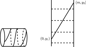
Figure 1. Twisting number

5.3. Twisting numbers of geodesics

Let $\beta\in\mathcal{S}$ with $\beta\neq\alpha$. For $t\in T$, we let $\beta^{*}_{t}$ be a geodesic representative of $\beta$ in $Y_{t}$ with respect to the $J_{t}$-metric. If $J_{t}$ admits a flat annulus whose core is homotopic to $\beta$, we choose one of the closed trajectories in the flat annulus to define $\beta^{*}_{t}$.

Let $\beta^{*}_{t}\cap A_{t}=\{\sigma^{1}_{s}\}_{s=1}^{n_{0}}$ be the set of $n_{0}$-straight line segments of $\beta^{*}_{t}$ that lie in $A_{t}$, counted with multiplicity. Notice that $n_{0}=i(\beta,\alpha)$, which is independent of the parameter $t$. Let $\{\sigma^{2}_{j}\}_{j}$ be a collection of maximal straight segments in $\beta^{*}_{t}\setminus\cup_{s=1}^{n_{0}}\sigma^{1}_{s}$, counting multiplicity. In this section, for a measured foliation $F$ and a path $\sigma$ transverse to the underlying foliation of $F$, we define $i(\sigma,F)$ to be the infimum of the integrals of the transversal measure of $F$ over all paths homotopic to $\sigma$ relative to endpoints.

Lemma 5.2 (Twisting number).

For $s=1,\cdots,n_{0}$, the twisting number of $\sigma^{1}_{s}$ in $A_{t}$ satisfies

$${\rm tw}_{A_{t}}(\sigma^{1}_{s})=o(K_{\gamma(t)})$$

as $t\to\infty$.

Proof.

When $n_{0}=i(\beta,\alpha)=0$, the geodesic representative $\beta^{*}_{t}$ does not intersect the interior of $A_{t}$. Hence, the conclusion automatically holds. Therefore, we may assume that $n_{0}\neq 0$.

Let $q_{t}=J_{t}/\|J_{t}\|$. Then, the vertical foliation $V_{q_{t}}$ of $q_{t}$ is equal to $\|J_{t}\|^{-1/2}\,G$ for all $t\in T$. In particular, the $q_{t}$-height $w_{t}$ of the characteristic annulus $A_{t}$ is equal to $\|J_{t}\|^{-1/2}\,w_{0}$. Let $H_{q_{t}}$ be the horizontal foliation of $q_{t}$. Since each $\sigma^{1}_{s}$ is a $q_{t}$-straight segment,

(5.1) $$i(\sigma^{j}_{s},V_{q_{t}})=\int_{\sigma^{j}_{s}}V_{q_{t}}\quad\mbox{and}\quad i(\sigma^{j}_{s},H_{q_{t}})=\int_{\sigma^{j}_{s}}H_{q_{t}}$$

for $j=1,2$. $i(\sigma^{j}_{s},V_{q_{t}})$ and $i(\sigma^{j}_{s},H_{q_{t}})$ are called the horizontal and vertical length of $\sigma^{j}_{s}$, respectively (cf. [23]).

Before giving the details, we first summarize the following calculation as follows. From Lemma 4.2, the width of the foliated annulus in $V_{q_{t}}$ of $\alpha$ is $\|J_{t}\|^{-1/2}w_{0}=K_{t}^{1/2}w_{0}+o(K_{t}^{1/2})$ as $t\to\infty$. Hence, from Lemma 5.1, the circumference $\ell_{t}$ of the characteristic annulus $A_{t}$ with respect to $q_{t}$ is comparable with $K_{t}^{-1/2}$. By Pythagoras’ theorem, the length of any component $\sigma^{j}_{s}$ is the square root of $K_{t}^{1/2}w_{0}+o(K_{t}^{1/2})$ and the vertical length $i(\sigma^{j}_{s},H_{J_{t}})$ in the characteristic annulus. From those observations and the assumption $\gamma(t)\to[G]$, we can deduce that the vertical length $i(\sigma^{j}_{s},H_{J_{t}})$ of $\sigma^{j}_{s}$ in the annulus with respect to $J_{t}$ tends to zero as (5.5) below. Therefore, from Lemma 4.2, the vertical length of $\sigma^{j}_{s}$ in the annulus with respect to $q_{t}$ is $o(K_{t}^{1/2})$. Thus, the twisting number is comparable with $i(\sigma^{j}_{s},H_{J_{t}})/\ell_{t}=o(K_{t})$ as $t\to\infty$ as desired.

Let us start the calculation. From the notation (5.1), by Pythagoras’ theorem, we have

(5.2) $$\ell_{q_{t}}(\beta^{*}_{t})=\sum_{s=1}^{n_{0}}\sqrt{i(\sigma^{1}_{s},H_{q_{t}})^{2}+i(\sigma^{1}_{s},V_{q_{t}})^{2}}+\sum_{j}\sqrt{i(\sigma^{2}_{j},H_{q_{t}})^{2}+i(\sigma^{2}_{j},V_{q_{t}})^{2}}.$$

Since $\|q_{t}\|=1$, we have $\ell_{q_{t}}(\beta^{*}_{t})\leq{\rm Ext}_{\gamma(t)}(\beta)^{1/2}$ from (2.1). Therefore,

$$\|J_{t}\|^{-1/2}i(\beta,G) =i(\beta,V_{q_{t}})\leq\ell_{q_{t}}(\beta^{*}_{t})$$

$$=\sum_{s=1}^{n_{t}}\sqrt{i(\sigma^{1}_{s},H_{q_{t}})^{2}+i(\sigma^{1}_{s},V_{q_{t}})^{2}}+\sum_{j}\sqrt{i(\sigma^{2}_{j},H_{q_{t}})^{2}+i(\sigma^{2}_{j},V_{q_{t}})^{2}}$$

$$=\sum_{s=1}^{n_{t}}\sqrt{i(\sigma^{1}_{s},H_{q_{t}})^{2}+\|J_{t}\|^{-1}\,w_{0}^{2}}+\sum_{j}\sqrt{i(\sigma^{2}_{j},H_{q_{t}})^{2}+i(\sigma^{2}_{j},V_{q_{t}})^{2}}$$

$$\leq{\rm Ext}_{\gamma(t)}(\beta)^{1/2}.$$

Thus, we obtain

$$i(\beta,G) \leq\sum_{s=1}^{n_{0}}\sqrt{\|J_{t}\|i(\sigma^{1}_{s},H_{q_{t}})^{2}+w_{0}^{2}}$$

$$\quad\quad+\sum_{j}\sqrt{\|J_{t}\|i(\sigma^{2}_{j},H_{q_{t}})^{2}+\|J_{t}\|i(\sigma^{2}_{j},V_{q_{t}})^{2}}$$

$$=\sum_{s=1}^{n_{0}}\sqrt{i(\sigma^{1}_{s},H_{J_{t}})^{2}+w_{0}^{2}}+\sum_{j}\sqrt{i(\sigma^{2}_{j},H_{J_{t}})^{2}+i(\sigma^{2}_{j},V_{J_{t}})^{2}}$$

(5.3) $$\leq\|J_{t}\|^{1/2}{\rm Ext}_{\gamma(t)}(\beta)^{1/2}.$$

From the assumption, Lemma 4.1 and (4.1),

$$\|J_{t}\|^{1/2}{\rm Ext}_{\gamma(t)}(\beta)^{1/2}=(1+o(1)){\rm Ext}_{\gamma(t)}(\beta)^{1/2}/K_{\gamma(t)}^{1/2}=(1+o(1))\mathcal{E}_{\gamma(t)}(\beta)$$

tends to $i(\beta,G)$ as $t\to\infty$. Since

$$i(\beta,G)=\int_{\beta^{*}_{t}}V_{J_{t}}=n_{0}w_{0}+\sum_{j}i(\sigma^{2}_{j},V_{J_{t}}),$$

we deduce from (5.3) that the sum

(5.4) $$\sum_{s=1}^{n_{0}} \left(\sqrt{i(\sigma^{1}_{s},H_{J_{t}})^{2}+w_{0}^{2}}-w_{0}\right)$$

$$\quad\quad+\sum_{j}\left(\sqrt{i(\sigma^{2}_{j},H_{J_{t}})^{2}+i(\sigma^{2}_{j},V_{J_{t}})^{2}}-i(\sigma^{2}_{j},V_{J_{t}})\right)$$

tends to zero as $t\to\infty$. Since every term in (5.4) is non-negative, we get

(5.5) $$\lim_{t\to\infty}i(\sigma^{1}_{s},H_{J_{t}})=0$$

for $s=1,\cdots,n_{0}$.

We now fix $s=1,\cdots,n_{0}$. Let $[0,w_{t}]\times\mathbb{R}\to[0,w_{t}]\times\mathbb{S}^{1}_{\ell_{t}}\cong A_{t}$ be the universal cover, where $\ell_{t}$ is the $q_{t}$-circumference of $A_{t}$. Let $(0,y_{1})$ and $(w_{t},y_{2})$ be the endpoints of a lift of $\sigma^{1}_{s}$. From the definition,

$$|y_{1}-y_{2}|=i(\sigma^{1}_{s},H_{q_{t}}).$$

Since

$${\rm Mod}(A_{t})=w_{t}/\ell_{t}=\|J_{t}\|^{-1/2}w_{0}/\ell_{t}=(1+o(1))K_{\gamma(t)}^{1/2}w_{0}/\ell_{t},$$

from Lemma 5.1, we obtain

(5.6) $$\ell_{t}\asymp K_{\gamma(t)}^{-1/2}$$

for $s=1,\cdots,n_{t}$. Thus, it follows from (5.5) that

$${\rm tw}_{A_{t}}(\sigma^{1}_{s}) =|y_{1}-y_{2}|/\ell_{t}\asymp i(\sigma^{1}_{s},H_{q_{t}})K_{\gamma(t)}^{1/2}$$

$$=\|J_{t}\|^{-1/2}i(\sigma^{1}_{s},H_{J_{t}})K_{\gamma(t)}^{1/2}=(1+o(1))i(\sigma^{1}_{s},H_{J_{t}})K_{\gamma(t)}$$

$$=o(K_{\gamma(t)}),$$

which implies what we wanted. ∎

5.4. Twisting deformations on flat annuli

In this section, we shall recall a canonical quasiconformal mapping of the twisting deformations along the core curve on a round annulus (cf. [24]).

Let $A=\{e^{-2\pi m}<|z|<1\}$ be a round annulus of modulus $m$. For $\tau>0$, we consider a quasiconformal self-mapping $W_{\tau}$ of $A$ by

$$W_{\tau}(z)=z|z|^{\frac{i\tau}{2\pi m}}.$$

Notice that $W_{\tau}$ satisfies

$$W_{\tau}\circ\Pi(x+iy)=\Pi\circ L(x+iy)$$

where $L(x+iy)=x+(\tau/m)y+iy$ and $\Pi:\{x+iy\mid 0\leq y\leq m\}\to A$ is the universal covering. Therefore, the Beltrami differential of $W_{\tau}$ is equal to

(5.7) $$\frac{\overline{\partial}W_{\tau}}{\partial W_{\tau}}=\frac{i(\tau/m)}{4\pi+i(\tau/m)}\frac{z}{\overline{z}}\frac{d\overline{z}}{dz}.$$

We can easily see that when a proper path $\sigma$ in $A$ has the twist parameter $\tau$, we can choose a sign $s\in\{+1,-1\}$ such that ${\rm tw}_{A}(W_{s\tau}(\sigma))=0$.

6. Proof of Theorem 1.2

In this section, we shall show Theorem 1.2. Throughout this section, we assume that $G=\Sigma_{i=1}^{k}w_{i}\alpha_{i}$ is a maximal rational foliation and $k=3g-3+m\geq 2$. Just as in the previous sections, we assume the projective class $[G]$ is the limit of an almost geodesic ray $\gamma:T\to T(X)$, and we continue to use the same notation.

6.1. Notation

Let $A_{i,t}\subset Y_{t}$ be the characteristic annulus of $q_{t}=J_{t}/\|J_{t}\|$ for $\alpha_{i}$. Let $\Sigma_{t}$ be the critical graph of $q_{t}$ and consider the $K_{\gamma(t)}^{-1/2}$-neighborhood $N_{t}$ of $\Sigma_{t}$ in $Y_{t}$ with respect to the $q_{t}$-metric. Let $A^{0}_{i,t}=A_{i,t}\setminus N_{t}$ (cf. Figure 2).

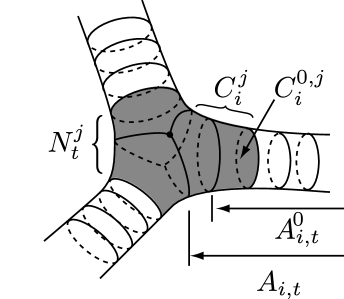
Figure 2. The vertical foliation of $q_{t}$ around a typical component of $N_{t}$. The component $N^{j}_{t}$ and annuli $C^{j}_{i}$, $C^{0,j}_{i}$ in the figure are taken and used in §6.3.2.

Since the $q_{t}$-height of $A_{i,t}$ is $(1+o(1))K_{\gamma(t)}^{1/2}w_{i}$, when $t\in T$ is sufficiently large, $A^{0}_{i,t}$ is a well-defined foliated subannulus of $A_{i,t}$ with height

(6.1) $$w^{\prime\prime}_{i,t}:=(1+o(1))K_{\gamma(t)}^{1/2}w_{i}-2K_{\gamma(t)}^{-1/2}\asymp K_{\gamma(t)}^{1/2}.$$

Let $\partial A^{0}_{i,t}=\partial_{1}A^{0}_{i,t}\cup\partial_{2}A^{0}_{i,t}$. Since $\partial A^{0}_{i,t}$ consists of closed leaves in $A_{i,t}$ and the heights of the remaining annuli in $A_{i,t}-A^{0}_{i,t}$ are at most $K_{\gamma(t)}^{-1/2}$, from (5.6), the moduli of remaining annuli in $A_{i,t}-A^{0}_{i,t}$ are uniformly bounded, and hence

$${\rm Mod}(A_{i,t})={\rm Mod}(A^{0}_{i,t})+O(1)$$

as $t\to\infty$.

6.2. Calculation of extremal length: Lower bound

Take $\beta\in\mathcal{S}$. We devote this section to bound the extremal length of $\beta$ from below. Henceforth, we suppose that $i(\beta,G)\neq 0$.

Let $\mathcal{A}_{t}^{\beta}$ be the characteristic annulus of the Jenkins-Strebel differential $J_{\beta,\gamma(t)}$ for $\beta$. Fix $i=1,\cdots,k$. The intersection $\mathcal{A}_{t}^{\beta}\cap A^{0}_{i,t}$ contains at least $n_{i}=i(\beta,\alpha_{i})$ components $\{D^{i}_{l}\}_{l=1}^{n_{i}}$ such that $D^{i}_{l}$ contains a path connecting $\mathcal{A}_{t}^{\beta}\cap\partial_{1}A^{0}_{i,t}$ and $\mathcal{A}_{t}^{\beta}\cap\partial_{2}A^{0}_{i,t}$.

Let $\Gamma(D^{i}_{l})$ be the family of rectifiable curves in $D^{i}_{l}$ connecting $\mathcal{A}_{t}^{\beta}\cap\partial_{1}A^{0}_{i,t}$ and $\mathcal{A}_{t}^{\beta}\cap\partial_{2}A^{0}_{i,t}$. Let $\rho^{i}_{t}$ be the restriction of the $q_{t}$-metric to $D^{i}=\cup_{i=1}^{n_{i}}D^{i}_{l}$. From (6.1), any curve in $\sum_{i=1}^{n_{i}}\Gamma(D^{i}_{l})$ has $\rho^{i}_{t}$-length at most $n_{i}w^{\prime\prime}_{i,t}$. Since the critical graph of the Jenkins-Strebel differential of $\beta$ on $Y_{t}$ has measure zero,

$$A(\rho^{i}_{t})=\iint_{D^{i}}\rho^{i}_{t}\leq(\mbox{$|q_{t}|$-area of $A^{0}_{i,t}$})=\ell_{i,t}w^{\prime\prime}_{i,t}.$$

By the definition of extremal length, we have

$${\rm Ext}\left(\sum_{i=1}^{n_{i}}\Gamma(D^{i}_{l})\right) \geq L_{\rho^{i}_{t}}\left(\sum_{i=1}^{n_{i}}\Gamma(D^{i}_{l})\right)^{2}/A(\rho^{i}_{t})\geq(n_{i}w^{\prime\prime}_{i,t})^{2}/\ell_{i,t}w^{\prime\prime}_{i,t}$$

$$=n_{i}^{2}{\rm Mod}(A^{0}_{i,t})=n_{i}^{2}{\rm Mod}(A_{i,t})+O(1).$$

Since any non-trivial simple closed curve in $\mathcal{A}_{t}^{\beta}$ traverses each $D^{i}_{l}$ between $\mathcal{A}_{t}^{\beta}\cap\partial_{1}A^{0}_{i,t}$ and $\mathcal{A}_{t}^{\beta}\cap\partial_{2}A^{0}_{i,t}$, such simple closed curve contains a curve in $\sum_{i=1}^{n_{i}}\Gamma(D^{i}_{l})$. Therefore, from (3) of Proposition 2.1, we conclude

(6.2) $${\rm Ext}_{\gamma(t)}(\beta)\geq\sum_{i=1}^{k}{\rm Ext}\left(\sum_{i=1}^{n_{i}}\Gamma(D^{i}_{l})\right)\geq\sum_{i=1}^{k}n_{i}^{2}{\rm Mod}(A_{i,t})+O(1)$$

as $t\to\infty$.

6.3. Calculation of extremal length: Upper bound

Before discussing the upper bound, we deform $Y_{t}$ slightly as follows. For $i=1,\cdots,k$, we fix a component $\sigma^{1}_{s_{i}}$ of $\beta^{*}_{t}\cap A_{i,t}$. We put the Beltrami differential (5.7) on each flat annulus $A_{i,t}$ with $\tau=\pm{\rm tw}_{A_{i,t}}(\sigma^{1}_{s_{i}})$ (we choose the appropriate sign so that the following holds). We extend the Beltrami differential to $Y_{t}$ by putting $0$ on the complement. Then, we obtain a quasiconformal deformation of $Y_{t}$ with respect to the Beltrami differential to get $\gamma^{\prime}(t)\in T(X)$. By Lemmas 5.1 and 5.2,

(6.3) $${\rm tw}_{A_{i,t}}(\sigma^{1}_{s_{i}})/{\rm Mod}(A_{i,t})\to 0$$

as $t\to\infty$ for all $i$, and hence,

$$d_{T}(\gamma(t),\gamma^{\prime}(t))\to 0$$

when $t\to\infty$. One can easily see that $\gamma^{\prime}:T\to T(X)$ is an almost geodesic ray. Furthermore, by Proposition 4.9 of [32], $\gamma^{\prime}(t)$ has the same limit as that of $\gamma(t)$ in the Gardiner-Masur compactification. Thus, to simplify of the notation, we may suppose that $\gamma^{\prime}(t)=\gamma(t)$.

As remarked in §5.4, if we choose the sign of $\tau$ suitably, after this deformation, the twist parameter of each $\sigma^{1}_{s_{i}}$ is zero. Hence, any segment in $\beta^{*}_{t}\cap A_{i,t}$ has the twisting number at most one in $A_{i,t}$ for all $i$, because $\beta$ is a simple closed curve and any two segments in $\beta^{*}_{t}\cap A_{i,t}$ do not intersect transversely in $A_{i,t}$. By taking a subray, we may assume that there is a (non-connected) graph $\Sigma_{0}$ on $X$ such that the marking $f_{t}:X\to Y_{t}$ induces an isomorphism $\Sigma_{0}$ and $\Sigma_{t}$ (in homotopy sense).

6.3.1. The idea for getting an appropriate upper bound

To bound of the extremal length from above, from (2.3), it suffices to construct a suitable annulus $\mathcal{A}_{t}$ on $Y_{t}$ whose core is homotopic to $f_{t}(\beta)$. The procedure given here is originally due to S. Kerckhoff in [16], when a given almost geodesic ray $\gamma$ is actually a geodesic (See also §9 of [26]). We briefly recall the construction in the case where $\gamma$ is a geodesic. We first cut each characteristic annulus $A_{i,t}$ of $J_{t}$ into $n_{i}=i(\beta,\alpha_{i})$ congruent horizontal rectangles. The annulus $\mathcal{A}_{t}$ is made by composing appropriately such (slightly modified) $n_{i}$ congruent horizontal rectangles and ties (quadrilaterals) in $N_{t}$ (cf. (6.5) and §6.3.2). We can take ties whose extremal lengths are uniform (cf. Lemma 6.1). Then, by applying Proposition 2.2, we obtain an upper bound of the extremal length of $\mathcal{A}_{t}$.

A basic reason why we can get an appropriate upper bound in the case above is that, along the Teichmüller ray associated to the projective class of $G=\sum_{i=1}^{k}w_{i}\alpha_{i}$, the characteristic annuli of the Jenkins-Strebel differential for $G$ are deformed with ‘no-twisting’ deformations, because the Teichmüller deformation is accomplished by stretching in the horizontal and vertical directions. In the upper bound, the major part comes from the extremal length of congruent rectangles (cf. (6.8)). The ‘no-twisting’ property implies that the totality of the extremal lengths of such rectangles coincides with the major part of the lower estimate (6.2) (see (6.7)).

In the case where $\gamma$ is an almost geodesic ray, we have already observed that $\beta$ is not twisted very much in the characteristic annuli (cf. (6.3)). Hence, we can apply the similar argument for getting an appropriate upper bound of ${\rm Ext}_{y_{t}}(\beta)$.

6.3.2. Ties $\{B^{j}_{s}\}_{s}$

In accordance with the idea explained above, we shall construct appropriate ties in pairs of pants $N_{t}^{j}$.

Since $G$ is maximal, any component $N^{j}_{t}$ ($j=1,\cdots,2g-2+m$) of $N_{t}$ is one of the three types: a pair of pants, an annulus with one distinguished point (a singularity of angle $\pi$ or a flat point), or a half-pillow with two cone singularities of angle $\pi$ (cf. Figure 3). We now assume that $N^{j}_{t}$ is a pair of pants because the case where $N^{j}_{t}$ is an annulus or a half-pillow can be dealt with in the same manner.

Notice from (5.6) that the length of any component of $\partial N^{j}_{t}$ is of order $K_{\gamma(t)}^{-1/2}$ with respect to the metric $\rho^{j}_{t}:=|q_{t}|_{N^{j}_{t}}$. For simplifying of the notation, we assume that components of $\partial N^{j}_{t}$ are $\alpha_{i_{1}}$, $\alpha_{i_{2}}$, and $\alpha_{i_{3}}$. Then, the critical graphs $\Sigma_{t}\cap N^{j}_{t}$ forms one of the graph in Figure 3 (cf. [6]).

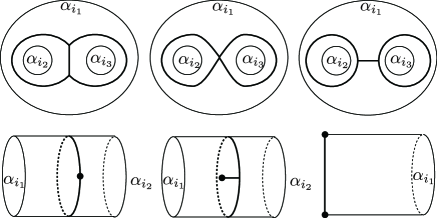
Figure 3. Graphs in $N^{j}_{t}$.

We make equally spaced $n_{i_{l}}$ cuts in $\alpha_{i_{l}}$ where $n_{i_{l}}=i(\beta,\alpha_{i_{l}})$ ($l=1,2,3$). Let $C^{j}_{i_{l}}$ be a component of $N^{j}_{t}\setminus\Sigma_{t}$ which contains $\alpha_{i_{l}}$ in the boundary. Let $C^{0,j}_{i_{l}}$ be a subannulus of $C^{j}_{i_{l}}$ with height $(2K_{\gamma(t)})^{-1/2}$ and $\alpha_{i_{l}}\subset C^{0,j}_{i_{l}}$. We cut $C^{0,j}_{i_{l}}$ along the vertical slits with endpoints in the $n_{i_{l}}$-cuts in $\alpha_{i_{l}}$ and get a family of Euclidean rectangles. Since the circumference and the height of $C^{0,j}_{i_{l}}$ are of order $(K_{\gamma(t)})^{-1/2}$, the moduli of such Euclidean rectangles are uniformly bounded above and below.

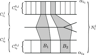
Figure 4. Typical examples of ties $B^{j}_{1}$ and $B^{j}_{2}$ in $N^{j}_{t}$. $B^{j}_{1}$ is a ‘regular’ quadrilateral and $B^{j}_{2}$ is a ‘singular’ quadrilateral.

The following lemma asserts that the contribution of the ties is small for the extremal length of the model annulus which will be constructed in (6.5) later.

Lemma 6.1 (See Figure 4).

There is a family $\{B^{j}_{s}\}_{s}$ of (singular) quadrilaterals such that

• $B^{j}_{s}\cap C^{0,j}_{i_{l}}$ is a rectangle above for all $s$ and $l$,

• the arc system given by correcting cores of $B^{j}_{s}$’s is homotopic to $\beta\cap N^{j}_{t}$, where the core of $B^{j}_{s}$ is a path in $B_{s}$ connecting facing arcs in $B^{j}_{s}\cap\partial N^{j}_{t}$ and

• the extremal length of the family of paths in $B^{j}_{s}$ homotopic to the core is uniformly bounded above.

Proof.

Notice from (5.6) and the uniformity of the moduli of $\{C^{j}_{i_{l}}\}_{l=1}^{3}$ that the conformal structure of $N^{j}_{t}$ is precompact in the reduced Teichmüller space of three holed spheres (cf. [7]). Since the intersection numbers $\{n_{i_{l}}\}_{l=1}^{3}$ are independent of $t$, we can take $B^{j}_{s}$ such that the width of each $B^{j}_{s}$ with respect to the $q_{t}$-metric are comparable with $K_{\gamma(t)}^{-1/2}$. By definition, the $|q_{t}|$-area of each $B^{j}_{s}$ is $O(K_{\gamma(t)}^{-1})$.

From the reciprocal relation between the module and the extremal length for quadrilateral or Rengel’s type inequality, the extremal length ${\rm Ext}(B^{j}_{s})$ of the family of paths in $B^{j}_{s}$ homotopic to the core satisfies

(6.4) $${\rm Ext}(B^{j}_{s})\leq\frac{\mbox{$|q_{t}|$-area}}{(\mbox{$|q_{t}|$-width})^{2}}=O(1)$$

for all $s$ (see §4 in Chapter I of [17]). ∎

6.3.3. Construction of a model $\mathcal{A}_{t}$ of the extremal annulus

We divide each $A_{i,t}$ into congruent $n_{i}=i(\beta,\alpha_{i})$ rectangles $\{R_{i,l}\}_{l=1}^{n_{i}}$ via proper horizontal segments. We may assume that for any $l$ and $j$, there is an $s$ such that $R_{i,l}\cap C^{0,j}_{i}$ is congruent to $B^{j}_{s}\cap C^{0,j}_{i}$. We set

$$R^{0}_{i,l}=R_{i,l}\setminus(N_{t}\setminus\cup_{j}C^{0,j}_{i})$$

(cf. Figure 5).

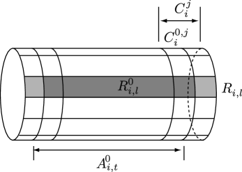
Figure 5. Rectangles $R_{i,l}$ and $R^{0}_{i,l}$ in the annulus $A_{i,t}$.

Since twisting numbers of segments in $\beta^{*}_{t}\cap A_{i,t}$ on each $A_{i,t}$ are at most one for all $i$, from (5.7) and the Dehn-Thurston’s parametrization of simple closed curves (cf. [6]), we can glue all $A_{i,t}$ and $N_{t}$ appropriately at the part $C_{i}^{0,j}$ to get a Riemann surface $Y^{\prime}_{t}$ and an annulus

(6.5) $$\mathcal{A}^{\prime}_{t}=(\cup_{i,l}R^{0}_{i,l})\cup(\cup_{j,s}B^{j}_{s}).$$

Since the moduli of the characteristic annuli diverge, after deforming $Y^{\prime}_{t}$ by a quasiconformal mapping with maximal dilatation $1+o(1)$, we obtain $Y_{t}$ and the core of the image $\mathcal{A}_{t}$ of the annulus $\mathcal{A}^{\prime}_{t}$ is homotopic to $f_{t}(\beta)$. Thus, we conclude

(6.6) $${\rm Ext}_{y_{t}}(\beta)={\rm Ext}_{Y_{t}}(f_{t}(\beta))\leq{\rm Ext}(\mathcal{A}_{t})=(1+o(1)){\rm Ext}(\mathcal{A}^{\prime}_{t})$$

as $t\to\infty$. Thus, to get the upper estimate of the extremal length of $\beta$ on $y_{t}$, it suffices to give an upper estimate of the extremal length of $\mathcal{A}^{\prime}_{t}$.

6.3.4. Estimate of extremal length of $\mathcal{A}^{\prime}_{t}$

Let $\rho^{\mathcal{A}}_{t}$ be the extremal metric on $\mathcal{A}^{\prime}_{t}$ for the extremal length ${\rm Ext}(\mathcal{A}^{\prime}_{t})$ with $A(\rho^{\mathcal{A}}_{t})=1$. Let $\{\mathcal{S}_{u}\}_{u}$ be a collection of all rectangles of the form $C^{0,j}_{i}\cap B_{s}^{j}$ for all $i,j,s$. By the same argument as Claim 1 in §9.6 in [26], we can see the following.

Claim 1.

For any $u$, there is a vertical line $\eta^{\prime}_{u}$ in $\mathcal{S}_{u}$ such that

$$\sum_{u}\ell_{\rho^{\mathcal{A}}_{t}}(\eta^{\prime}_{u})=O(1)$$

as $t\to\infty$.

Let us continue the calculation. Let $\{D_{u}\}_{u}$ be a collection of components of $\mathcal{A}^{\prime}_{t}\setminus\cup_{u}\eta^{\prime}_{u}$. By labeling correctly, we may assume that $\partial D_{u}$ contains $\eta^{\prime}_{u}$ and $\eta^{\prime}_{u+1}$, where $\eta^{\prime}_{u}$ is labeled cyclically in $u$. By definition, each $D_{u}$ is contained in either $R_{i,l}$ or $B^{j}_{s}$ for some $i,l,j,s$. Let $\Gamma(D_{u})$ be the family of rectifiable paths connecting vertical segments $\eta^{\prime}_{u}$ and $\eta^{\prime}_{u+1}$. Let $\Gamma(R_{i,l})$ be the family of rectifiable paths in $R_{i,l}$ connecting vertical boundary segments. Since

(6.7) $${\rm Ext}(\Gamma(R_{i,l}))=(\mbox{the height of $A_{i,t}$})/(\ell_{i,t}/n_{i})=n_{i}{\rm Mod}(A_{i,t}),$$

by (1) and (2) of Proposition 2.2 and Claim 1, we have

$${\rm Ext}(\mathcal{A}^{\prime}_{t})^{1/2} =\left(\sum_{u}{\rm Ext}(\Gamma(D_{u}))\right)^{1/2}+O(1)$$

$$\leq\left(\sum_{D_{u}\subset R_{i,l}}{\rm Ext}(\Gamma(R_{i,l}))+\sum_{D_{u}\subset B^{j}_{s}}{\rm Ext}(B^{j}_{s})\right)^{1/2}+O(1)$$

$$\leq\left(\sum_{D_{u}\subset R_{i,l}}n_{i}{\rm Mod}(A_{i,t})+O(1)\right)^{1/2}+O(1)$$

(6.8) $$=\left(\sum_{i=1}^{k}n_{i}^{2}{\rm Mod}(A_{i,t})+O(1)\right)^{1/2}+O(1).$$

Thus we get the desired upper bound of the extremal length of $\mathcal{A}^{\prime}_{t}$, and hence of ${\rm Ext}_{y_{t}}(\beta)$ from (6.6).

6.4. Conclusion

From Lemma 5.1, by taking a subray if necessary, we may assume that ${\rm Mod}(A_{i,t})/K_{\gamma(t)}$ tends to a positive number $M_{i}$ for each $i=1,\cdots,k$. From (6.2), (6.6), and (6.8), we deduce that

(6.9) $$i(\beta,G)=\lim_{t\to\infty}\left(\frac{{\rm Ext}_{\gamma(t)}(\beta)}{K_{\gamma(t)}}\right)^{1/2}=\left(\sum_{i=1}^{k}n_{i}^{2}M_{i}\right)^{1/2}=\left(\sum_{i=1}^{k}M_{i}i(\beta,\alpha_{i})^{2}\right)^{1/2}$$

for all $\beta\in\mathcal{S}$. Since the set $\mathbb{R}_{+}\otimes\mathcal{S}$ of the weighted simple closed curves is dense in $\mathcal{MF}$, and the intersection number function is continuous and homogeneous on the product $\mathcal{MF}\times\mathcal{MF}$, the above equation (6.9) still holds for all measured foliations $\beta\in\mathcal{MF}$. Thus, for any $x,y>0$ and $\beta_{1},\beta_{2}\in\mathcal{S}$ with $i(\beta_{1},\beta_{2})=0$, by substituting $\beta=x\beta_{1}+y\beta_{2}$ to (6.9), we get

$$\left(\sum_{i=1}^{k}M_{i}n_{1,i}^{2}\right)x^{2} +2\left(\sum_{i=1}^{k}M_{i}n_{1,i}n_{2,i}\right)xy+\left(\sum_{i=1}^{k}M_{i}n_{2,i}^{2}\right)y^{2}$$

$$=(xi(\beta_{1},G)+yi(\beta_{2},G))^{2},$$

where $n_{j,i}=i(\beta_{j},\alpha_{i})$. This means that the discriminant of the quadratic form above is zero. Namely, we have

$$\left(\sum_{i=1}^{k}M_{i}n_{1,i}n_{2,i}\right)^{2}-\left(\sum_{i=1}^{k}M_{i}n_{1,i}^{2}\right)\left(\sum_{i=1}^{k}M_{i}n_{2,i}^{2}\right)=0,$$

for all such pair of curves $\beta_{1},\beta_{2}\in\mathcal{S}$. Hence, two vectors

$$(\sqrt{M_{1}}n_{1,1},\cdots,\sqrt{M_{k}}n_{1,k}),\quad(\sqrt{M_{1}}n_{2,1},\cdots,\sqrt{M_{k}}n_{2,k}),$$

are parallel for all $\beta_{1},\beta_{2}\in\mathcal{S}$ with $i(\beta_{1},\beta_{2})=0$. However, this is impossible when $k=3g-3+m\geq 2$, as we already observed in Section 7 of [26].

References

- [1] L. V. Ahlfors, Lectures on Quasiconformal Mappings, Van Nostrand Mathematical Studies, vol. 10. D. Van Nostrand Co., Inc., Toronto, Ont.-New York-London (1966) .
- [2] L. V. Ahlfors, Conformal invariants: Topics in Geometric Function Theory, McGrow-Hill, NewYork (1973).
- [3] M. Akian, S. Gaubert, and C. Walsh, The Max-Plus Martin boundary, Documenta Math., 14 (2009), 195–240.
- [4] L. Bers, Quasiconformal mappings and Teichmüller’s theorem, in Analytic Functions, Princeton University Press, Princeton, N. J. (1960), 89–119.
- [5] M. Bridson and A. Haefliger, Metric spaces of Non-positive curvature, Grundlehren der mathematischen Wissenschaften 319, Springer Verlag (1999).
- [6] A. Douady, A. Fathi, D. Fried, F. Laudenbach, V. Poénaru, and M. Shub, Travaux de Thurston sur les surfaces, Séminaire Orsay (seconde édition). Astérisque No. 66-67, Société Mathématique de France, Paris (1991).
- [7] C. Earle, Reduced Teichmüller spaces, Trans Amer. Math. Soc. 126 (1967), 54–63.
- [8] F. Gardiner, Measured foliations and the minimal norm property for quadratic differentials, Acta Math. 152 (1984), no. 1-2, 57–76.
- [9] F. Gardiner and H. Masur, Extremal length geometry of Teichmüller space. Complex Variables Theory Appl. 16 (1991), no. 2-3, 209–237.
- [10] M. Gromov, Hyperbolic manifolds, groups and actions, In Riemann surfaces and related topics, Proceedings of the 1978 Stony Brook Conference, 182–213, Princeton University Press (1981).
- [11] J. Hubbard, and H. Masur, Quadratic differentials and foliations, Acta Math. 142 (1979), no. 3-4, 221–274.
- [12] Y. Imayoshi and M. Taniguchi, Introduction to Teichmüller spaces, Springer-Verlag (1992).
- [13] V. Kaimanovich and H. Masur, The Poisson boundary of the Mapping class group, Invent. Math. 125 (1996), 221–264.
- [14] V. Kaimanovich and H. Masur, The Poisson boundary of Teichmüller space, Jour. Funct. Anal. 156 (1998), 301–332.
- [15] A. Karlsson, V. Metz and G. A. Noskov, Horoballs in simplices and Minkowski space, Int. J. Math. Math. Sci., (2006), Art. ID 23656.
- [16] S. Kerckhoff, The asymptotic geometry of Teichmüller space, Topology 19 (1980), 23–41.
- [17] O. Lehto and K. Virtanen, Quasiconformal mappings in the plane, Second edition, Die Grundlehren der mathematischen Wissenschaften, Band 126. Springer-Verlag, New York-Heidelberg, (1973).
- [18] L. Liu, A. Papadopoulos, W. Su and G. Théret, Length spectra and the Teichmüller metric for surfaces with boundary, Monatsh Math 161, 295–311 (2010).
- [19] L. Liu and W. Su, The horofunction compactification of Teichmüller metric, preprint, ArXiv.org : http://arxiv.org/abs/1012.0409.
- [20] A. Marden, and K. Strebel, The height theorem for quadratic differentials on Riemann surfaces, Acta. Math 153 (1984), 153–211.
- [21] H. Masur, On a class of geodesics in Teichmüller space. Ann. of Math. 102 (1975), 205–221.
- [22] H. Masur, Random walks on Teichkmüller space and the mapping class group, J. Anal. Math. 67 (1995), 117–164.
- [23] H. Masur and Y. Minsky, Geometry of the complex of curves, I: Hyperbolicity, Invent. Math. 138 (1999), 103–149.
- [24] A. Marden and H. Masur, A foliation of Teichmüller space by twist invariant disks, Math. Scand. 36 (1975), 211–228.
- [25] H. Miyachi, On the Gardiner-Masur boundary of Teichmüller spaces Proceedings of the 15th ICFIDCAA Osaka 2007, OCAMI Studies 2 (2008), 295–300.
- [26] H. Miyachi, Teichmüller rays and the Gardiner-Masur boundary of Teichmüller space. Geom. Dedicata 137 (2008), 113–141.
- [27] H. Miyachi, Teichmüller rays and the Gardiner-Masur boundary of Teichmüller space II, Geom. Dedicata 162 (2013), 283–304.
- [28] H. Miyachi, Unification of extremal length geometry on Teichmüller space via intersection number, submitted.
- [29] Y. Minsky, Teichmüller geodesics and ends of hyperbolic 3-manifolds. Topology 32, 625–647 (1993).
- [30] Y. Minsky, Extremal length extimates and product regions in the Teichmüller space, Duke Math. J. 83 (1996) 249–286.
- [31] A. Papadopoulos, Problem 13 in Problem Session “Teichmüller Theory”, Oberwolfach Reports Vol. 7, (2010) Issue 4, 3085–3157.
- [32] M. Rieffel, Group -algebras as compact quantum metric spaces, Documenta Math. 7 (2002), 605–651.
- [33] K. Strebel, Quadratic Differentials, Springer Verlag, Berlin and New York (1984).
- [34] C. Walsh, The horofunction boundary of the Hilbert geometry, Advanced in Geometry 8, 503–529 (2008).
- [35] C. Walsh, The horoboundary and isometry group of Thurson’s Lipschitz metric, preprint, ArXiv.org : http://arxiv.org/abs/1006.2158
- [36] C. Walsh, The asymptotic geometry of the Teichmüller metric, preprint. (2012).
- [37] C. Webster and A. Winchester, Busemann points of infinite graphs, Trans. Amer. Math. Soc. 358 (2006), 4209–4224.