Black Holes in Braneworld Models

Abstract

In this review, we summarize current understandings of black hole solutions in various braneworld models, including the Arkani-Hamed-Dimopoulos-Dvali model, the Randall-Sundrum (RS) models, Karch-Randall (KR) model and the Dvali-Gabadadze-Porrati model. After illustrating basic properties of each braneworld model, we introduce the bulk/brane correspondence in the RS and KR braneworld models, adding supporting evidence for it. We then summarize the studies on braneworld black hole solutions, which consist of constructing exact or approximate solutions and investigating the phase diagram of solutions. In the study of phase diagram, we will also expound the implications of the bulk/brane correspondence to the braneworld black holes.

1 Introduction

Contemporary candidates of quantum gravity, such as string theory or M-theory, predict that our spacetime is higher-dimensional even though we observe seemingly four-dimensional world. To reconcile this apparent conflict in the spacetime dimensionality, we have to introduce some mechanisms into the spacetime structure. One of such mechanisms is the Kaluza-Klein (KK) compactification [1, 2], in which extra dimensions are manifestly compactified into a finite size manifold. Another one is the braneworld model, which we will focus on in this review.

A braneworld models is composed of higher-dimensional bulk spacetime and lower-dimensional brane in it. Standard model particles are confined onto the brane but gravity is allowed to propagate in the bulk. These models are partly motivated by string theory in the following sense. In string theory, membrane-like solutions emerge as a result of string condensation. Open strings attached on this membrane will behave as matter fields confined on it. Closed strings, on the other hand, can freely move away from the brane, and will behave as graviton propagating in the bulk. The braneworld models will capture gravitational aspect of such membrane-like solutions.

Since graviton propagates in the bulk and then the gravity in this model is higher-dimensional, we need some mechanisms to recover the four-dimensional gravity on the brane. The simplest way would be cutting off the extra dimensions in a manner similar to the Kaluza-Klein compactification. In the Arkani-Hamed-Dimopoulos-Dvali (ADD) model [3, 4], the first braneworld model, and in the Randall-Sundrum I (RS-I) model [5], the four-dimensional gravity is recovered in this way. Second way is to introduce the so-called warped compactification, with which we can localize the gravity onto the brane even when the bulk extends infinitely. This mechanism is used in the Randall-Sundrum II (RS-II) model [6], which is composed of negatively curved bulk spacetime and a four-dimensional brane with tension. Yet another way to localize gravity is to manifestly introduce the four-dimensional Einstein-Hilbert action localized on the brane, which is adopted in the Dvali-Gabadadze-Porrati (DGP) model [7].

These gravity localization mechanisms can be assessed by perturbation analyses in the weak gravity regime, and indeed they are shown to work well. In the strong gravity regime, however, it is not clear how the gravity behaves due to complexity of the Einstein equations. Especially, the properties of black hole solutions in braneworld models are not yet fully understood though much effort has been devoted to this issue. In this chapter, we will review current understanding about such black hole solutions in braneworld models.

As for the RS braneworld model, there is another noteworthy point. Since its unperturbed bulk spacetime is anti-de Sitter (AdS) space, it is expected that the AdS/CFT correspondence [8, 9] applies also to this model [10, 11]. The AdS/CFT correspondence indicates the duality between classical gravity in the bulk and conformal field theory on the AdS boundary. A novel feature of the duality in the RS model is that the quantum theory on the boundary couples to gravity, while they are decoupled in the original AdS/CFT correspondence. Even though there is no direct proof for this modified duality so far, a vast number of works are supporting it. This bulk/brane correspondence in braneworld models will be a topic that we focus on in this review.

This chapter is organized as follows. We firstly review in §2 the basics of braneworld models, such as their geometrical structure and properties of weak gravity on it. In §3, we introduce the effective Einstein equations on the brane and the bulk/brane correspondence in the RS braneworld model. Next, we discuss black holes in the ADD model in §4, and those in the RS model in §5, mainly focusing on brane-localized black holes. Since even a numerical solution describing a large brane-localized black hole in the RS model has not been found so far, we begin with the predictions derived from the bulk/brane correspondence. After that, we summarize the progress in studies on the brane-localized black holes and give arguments supporting the predictions. We will also discuss the studies on black hole solutions in other braneworld models, including the Karch-Randall (KR) model and the DGP model, in §6. Finally, we will briefly summarize this review and mention some prospects in §7.

Notations and Conventions

In this chapter, we express the metric in the bulk as $g_{AB}$ with indices $A,B,\dots$, and covariant derivative with respect to $g_{AB}$ as ${\rm NewA}_{A}$. Correspondingly, we express the metric on the brane and covariant derivative with respect to it as $\gamma_{\mu\nu}$ and $D_{\mu}$ with indices $\mu,\nu,\dots$ . We use indices $i,j,\dots$ for coordinates in the spatial direction when necessary.

2 Braneworld models

Braneworld models are higher-dimensional spacetime models in which the standard model particles are confined on a four-dimensional hypersurface (brane) while gravity can freely propagate in the higher-dimensional spacetime (bulk) which encompass the brane. The first braneworld model is the ADD model with tensionless brane and compactified flat extra dimensions. Later, this model is extended to the RS model that consists of non-zero tension branes and a warped, i.e., negatively curved bulk spacetime. Another variation of braneworld model is to include the Einstein-Hilbert action localized on the brane, which is called the DGP model. This model leads to gravity modification in a long distance scale while keeping the ordinary Einstein gravity in a short distance scale.

In this section, we introduce these braneworld models and explain the behaviors of weak gravity in these models. Starting with a brief introduction of the ADD model in §2.1, we explain the RS model in §2.2. We also introduce a variant of the RS model with an asymptotically AdS brane, which is called the KR model, in §2.3. Finally, we mention the DGP model in §2.4.

2.1 ADD model

The prototype of current braneworld models is the ADD model [3, 4], which is composed of a tensionless brane and flat compactified extra dimensions. This model was introduced to resolve the hierarchy problem between the Planck scale $M_{\text{Pl}}\sim 10^{19}\,\mathrm{GeV}$ and the electroweak scale $M_{\text{EW}}\sim 1\,\mathrm{TeV}$ (see Refs. Kribs:2006mq and Cheng:2010pt about particle physics studies in this model, and Ref. Antoniadis:1998ig about embedding of the model into string theory).

The action of gravity in $(4+d)$-dimensions is assumed to be simply given by Einstein-Hilbert action

$$S={1\over 16\pi G_{4+d}}\int d^{4}x\int d^{d}y\sqrt{-g}\,R~{},$$ (1)

where $R$ is the curvature scalar in $(4+d)$-dimensions. As in the case of Kaluza-Klein compactification, modes which have non-trivial structure in the directions of extra dimensions are massive. Hence, they are difficult to excite. Neglecting these massive excitations, we assume that the configuration is homogeneous in $y$-directions. Under this assumption, we can integrate over extra dimensions to obtain

$$S\approx{L^{d}\over 16\pi G_{4+d}}\int d^{4}x\sqrt{-g^{(4)}}\,R^{(4)}~{},$$ (2)

where $g^{(4)}_{\mu\nu}$ is the metric on a four-dimensional section, and $R^{(4)}$ is scalar curvature computed from $g^{(4)}_{\mu\nu}$. $L^{d}$ is the $d$-dimensional volume of extra dimensions.

Comparing the reduced action (2) with the four-dimensional Einstein-Hilbert action, $S_{4D}={1\over 16\pi G_{4}}$ $\int d^{4}x\sqrt{-g^{(4)}}R^{(4)}$, we find that the effective four-dimensional Planck mass $M_{4}=G_{4}^{-1/2}$ is related to the original $(4+d)$-dimensional one $M_{4+d}=G_{4+d}^{-1/(2+d)}$ by

$$M_{pl}^{2}\approx M_{4+d}^{2+d}L^{d}~{}.$$ (3)

Then, for $M_{4}\sim 10^{19}\,\mathrm{GeV}$, $M_{4+d}$ is given as $M_{4+d}\sim 10^{\frac{38-15d}{2+d}}\times\left(\frac{0.1\mathrm{mm}}{L}\right)^{\frac{d}{2+d}}\mathrm{GeV}$, and $M_{4+d}$ becomes as low as TeV if we set $d=2$ and $L\sim 0.1\,\mathrm{mm}$. Note that this relatively large extra dimension scale will not be probed by high energy particle experiments since the standard model particles are confined on the brane. The model with $d=1$ is already excluded since $L$ must be astrophysical distance scale, while the models with $d\geq 3$ are observationally allowed for a wide range of model parameters. Since the brane is tensionless in this model, the gravitational property of this model is similar to that of a KK compactified spacetime. Namely, long distance behavior of gravity is similar to the four-dimensional one with the effective gravitational coupling mentioned above, while at a short distance comparable to the size of extra dimensions the gravity becomes higher-dimensional.

2.2 RS model

The RS model is a braneworld model composed of branes with tension and a warped bulk spacetime with a negative cosmological constant. The first model with a bulk bounded by positive and negative tension branes was introduced in Ref. RS-I to give an alternative viewpoint to the hierarchy problem. Later, another variation of this model was proposed, in which the negative tension brane was sent to infinity [6]. These models are called the RS-I and RS-II models, respectively. We will explain basic features of gravity in these models below.

2.2.1 RS-I model

The unperturbed background of the RS-I model is composed of a five-dimensional AdS bulk bounded by a positive tension brane located on the AdS boundary side and a negative tension brane on the other side. Its action is given by

$$S_{\text{RS-I}} = \frac{1}{16\pi G_{5}}\int\!d^{5}x\sqrt{-g}\left(R-2\Lambda_{5}\right)$$ (5)

$$-\int\!dyd^{4}x\sqrt{-\gamma}\left\{(\lambda_{+}+L_{m+})\delta\left(y\right)+(\lambda_{-}+L_{m-})\delta\left(y-y_{-}\right)\right\}~{},$$

where $y$ is the spatial coordinate in the bulk direction, and $\gamma_{MN}$ is four-dimensional induced metric on $y=\text{constant}$ surfaces. The AdS boundary is at $y=-\infty$, and the brane with positive and negative tension are located at $y=0$ and $y=y_{-}>0$, respectively. We impose $Z_{2}$-symmetry about the branes to the spacetime. In other words, we require that the spacetime has reflection symmetry about the branes. $L_{\pm}$ is the Lagrangian of the matter fields localized on the respective branes. The bulk spacetime is characterized by its curvature length $\ell$, which is related to the five-dimensional cosmological constant $\Lambda_{5}$ by $\Lambda_{5}=-6/\ell^{2}$. The brane tensions $\lambda_{\pm}$ are set to

$$\lambda_{+}=-\lambda_{-}=\frac{3}{4\pi G_{5}\ell}$$ (6)

so as to be compatible with a four-dimensional Minkowski spacetime on each brane. Then, the five-dimensional Einstein equations are given by

$$R_{MN}-\frac{1}{2}Rg_{MN} = -\Lambda_{5}g_{MN}-8\pi G_{5}\Bigl{\{}(\lambda_{+}\gamma_{MN}+\tau_{+MN})\delta\left(y\right)$$ (8)

$$\qquad\qquad\qquad\qquad+(\lambda_{-}\gamma_{MN}+\tau_{-MN})\delta\left(y-y_{-}\right)\Bigr{\}}~{},$$

where $\tau_{\pm MN}$ are the energy momentum tensors of the matter fields localized on the branes. The delta functions on the right-hand side originate from the terms localized on the branes. Integrating this equation for an infinitesimal range across the brane, junction conditions at the brane are obtained as (see also §3.1 for an alternative derivation)

$$\left[K^{\pm}_{\mu\nu}-K^{\pm}\gamma_{\mu\nu}\right]^{+}_{-}=8\pi G_{5}(\lambda_{\pm}\gamma_{\mu\nu}+\tau_{\pm\mu\nu})~{},$$ (9)

where $K^{\pm}_{\mu\nu}\equiv-\gamma_{\mu}^{~{}M}\gamma_{\nu}^{~{}N}{\rm NewA}_{M}s^{\pm}_{N}$ is the extrinsic curvature and $s^{M}_{\pm}$ are the unit normal vectors of the respective branes. The notation $[f(y)]^{+}_{-}$ represents $f(y\to y_{b}+0)-f(y\to y_{b}-0)$ with $y_{b}$ being the location of the brane. A simplest solution to these equations is given by

$$ds^{2}=e^{2|y-y_{-}|/\ell}\eta_{\mu\nu}dx^{\mu}dx^{\nu}+dy^{2}~{},$$ (10)

where $\eta_{\mu\nu}$ is four-dimensional Minkowski metric. Since the standard model particles are supposed to be confined on the negative tension brane, we normalized the warp factor $e^{2|y-y_{-}|/\ell}$ so as to be unity there.

Notice that the above solution (10) remains to be a solution even if the four-dimensional Minkowski metric $\eta_{\mu\nu}$ is replaced with any metric that solves the four-dimensional vacuum Einstein equations. Hence, substituting this simple metric form (the one with $\eta_{\mu\nu}$ replaced with a generic four-dimensional metric), the five-dimensional gravitational action is reduced to an effective four-dimensional one. From this reduction, we can easily read that the effective four-dimensional Planck mass $M_{4}=G_{4}^{-1/2}$ is related to the five-dimensional one $M_{5}=G_{5}^{-1/3}$ as

$$M_{4}^{2}=\ell M_{5}^{3}\left(e^{2y_{-}/\ell}-1\right)~{}.$$ (11)

If we set the brane position at $y_{-}/\ell\sim 37$, the energy scale in five dimensions are unified as $\ell^{-1}\sim M_{5}\sim 1\,\mathrm{TeV}$. Namely, we can absorb the energy hierarchy between the Planck scale and the electroweak scale into the geometrical hierarchy of $\mathcal{O}(10)$ in the RS-I model. The particle phenomenology in this model was widely discussed [12].

2.2.2 RS-II model

Let us take the limit of sending the negative tension brane to infinity ($y_{-}\to\infty$) in the RS-I model, and suppose that we are living on the positive tension brane. Then, we obtain a model with one positive tension brane whose unperturbed metric is given by

$$ds^{2}=g^{(0)}_{MN}dx^{M}dx^{N}=e^{-2|y|/\ell}\eta_{\mu\nu}dx^{\mu}dx^{\nu}+dy^{2}=\frac{\ell^{2}}{\left(|z|+\ell\right)^{2}}\left(\eta_{\mu\nu}dx^{\mu}dx^{\nu}+dz^{2}\right)~{},$$ (12)

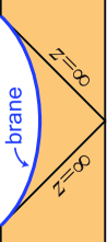
Figure 1: Conformal diagram of the RS model.

where we introduced a conformal coordinate $z\equiv\text{sign}(y)\ell(e^{|y|/\ell}-1)$. In this case the effective four-dimensional Planck mass is given by $M_{4}^{2}=\ell M_{5}^{3}$ (or equivalently $G_{4}=G_{5}/\ell$), and then this model is not useful to solve the hierarchy problem.

An interesting point of this model is that the higher-dimensional gravity is effectively confined around the brane, although the extra dimension is infinitely extending. The conformal diagram of this spacetime is depicted in Fig. 1. Thanks to the warping of the bulk spacetime and so-called volcano type gravitational potential due to the brane, which is given by Eq. (15) below, the five-dimensional gravity is localized on the brane and an approximate four-dimensional gravity is realized on it. This perturbative analysis on the gravity in the RS model was done in Ref. Garriga:1999yh.

It is convenient to work in the so-called RS gauge, which is defined for the metric perturbation $h_{MN}\equiv g_{MN}-g^{\text{(0)}}_{MN}$ by

$$h_{zz}=0=h_{\mu z}\,,\quad h_{\mu}^{~{}\,\nu}{}_{,\nu}=0\,,\quad h^{\mu}_{~{}\mu}=0\,.$$ (13)

In this gauge, the equation of motion for the metric perturbation is simply given by

$$\left[-\partial_{z}^{2}+V(z)\right]\psi_{\mu\nu}=\eta^{\rho\lambda}\partial_{\rho}\partial_{\lambda}\psi_{\mu\nu}~{},$$ (14)

where $\psi_{\mu\nu}\equiv\sqrt{|z|+\ell}\,h_{\mu\nu}$ and

$$V\left(z\right)=\frac{15}{4\left(\left|z\right|+\ell\right)^{2}}-3\ell^{2}\delta\left(z\right)~{}.$$ (15)

Separating the variables as $\psi_{\mu\nu}\propto\hat{u}_{m}(z)e^{ik_{\lambda}x^{\lambda}}$, we obtain an eigenvalue equation

$$\left[-\partial_{z}^{2}+V(z)\right]\hat{u}_{m}(z)=m^{2}\hat{u}_{m}(z)~{},$$ (16)

where $m^{2}=-k_{\mu}k^{\mu}$ is the effective four-dimensional mass of the mode $\hat{u}_{m}(z)$. The general solution that satisfies $Z_{2}$-symmetry about the brane is given in terms of the Bessel functions as

$$\hat{u}_{m}(z)=N_{m}\sqrt{|z|+\ell}\left[J_{1}(m\ell)Y_{2}\bigl{\{}m(|z|+\ell)\bigr{\}}-Y_{1}(m\ell)J_{2}\bigl{\{}m(|z|+\ell)\bigr{\}}\right]~{},$$ (17)

where $N_{m}\equiv\left(m/2\right)^{1/2}\left\{J_{1}(m\ell)^{2}+Y_{1}(m\ell)^{2}\right\}^{-1/2}$ is the normalization constant which is determined from the requirement $2\int_{\ell}^{\infty}\hat{u}_{m}(z)\hat{u}_{m^{\prime}}(z)dz=\delta(m-m^{\prime})$. Besides these modes, there is a discrete mass spectrum at $m^{2}=0$ with the wave function $\hat{u}_{0}(z)=\ell(|z|+\ell)^{-3/2}$, which is called “zero mode”. This zero mode wave function is nodeless. Since Eq. (16) is an eigenvalue equation of Schrödinger type, the nodeless solution is the mode with the lowest eigenvalue. Therefore there is no bound state with $m^{2}<0$.

From these mode functions, we obtain Green’s function for $-\partial_{z}^{2}+V(z)$ as

$$\hat{G}({\bm{x}},z,{\bm{x}^{\prime}},z^{\prime})\\ \quad=-\!\!\int_{-\infty}^{\infty}\!\!dt\!\!\int\!\!\frac{d^{4}k}{(2\pi)^{4}}e^{ik_{\mu}\left(x^{\mu}-x^{\prime\mu}\right)}\!\!\left[\frac{\hat{u}_{0}(z)\hat{u}_{0}(z^{\prime})}{{\bm{k}}^{2}-(\omega+i\epsilon)^{2}}+\int_{0}^{\infty}\!\!\!dm\frac{\hat{u}_{m}(z)\hat{u}_{m^{\prime}}(z^{\prime})}{m^{2}+{\bm{k}}^{2}-(\omega+i\epsilon)^{2}}\right],$$ (18)

and the Green function for $h_{\mu\nu}$ is given by $G=\ell(|z|+\ell)^{-1/2}(|z^{\prime}|+\ell)^{-1/2}\hat{G}$. In the RS gauge, however, the brane moves from its original position when gravitational sources exist on the brane. To obtain the induced metric on the brane, we have to transform the coordinates into the the ones in which the brane is located at $\bar{y}=0$, where bar “$~{}\bar{}~{}$” is associated for the distinction from the quantities in the original coordinates. We further require $\bar{h}_{zz}=0=\bar{h}_{z\mu}$, and we conventionally call them Gaussian-normal coordinates. Then, we obtain the induced metric components for a spherical source of mass $M$ on the brane as [15]

$$\bar{h}_{tt}=\frac{2G_{4}M}{r}\left(1+\frac{2\ell^{2}}{3r^{2}}\right)~{},\qquad\bar{h}_{ij}=\frac{2G_{4}M}{r}\left(1+\frac{\ell^{2}}{3r^{2}}\right)\delta_{ij}~{}.$$ (19)

This $\bar{h}_{tt}$ is nothing but the modified Newton potential for the source $M$. The metric perturbation in the bulk generated by a static source on the brane is summarized by [15]

$$G({\bm{x}},z,{\bm{x}^{\prime}},0)\simeq-\frac{\ell}{8\pi z^{2}}\frac{2r^{2}+3z^{2}}{\left(r^{2}+z^{2}\right)^{3/2}}~{},$$ (20)

which implies that the metric perturbation in the asymptotic region behaves as $\mathcal{O}(r^{-1})$ for a large $r$ and $\mathcal{O}(z^{-3})$ for a large $z$.

2.3 KR model

We saw that the five-dimensional gravity is localized onto the brane in the RS-II model due to the bulk spacetime warping. Karch and Randall found that this feature persists even when the brane tension is detuned and the four-dimensional spacetime on the brane becomes asymptotically AdS spacetime. This model with asymptotically AdS branes was firstly proposed as an extension of the RS-II model in Ref. KR, and its embedding to the string theory was discussed later in Refs. KRstring_orig,KRstring,DeWolfe,DeWolfe2. We briefly explain this KR braneworld model below.

Starting with the RS-II model, we decrease the brane tension as

$$\lambda=\frac{3(1+\delta)}{4\pi G_{5}\ell}~{},$$ (21)

with $\delta<0$. Then, the unperturbed five-dimensional metric for this model becomes

$$ds^{2}=\frac{\ell^{2}}{L^{2}\sin^{2}\left\{(|z|+z_{0})/L\right\}}\left(\gamma_{\mu\nu}dx^{\mu}dx^{\nu}+dz^{2}\right)~{},$$

$$\gamma_{\mu\nu}dx^{\mu}dx^{\nu}=-\left(1+\frac{r^{2}}{L^{2}}\right)dt^{2}+\frac{dr^{2}}{1+\frac{r^{2}}{L^{2}}}+r^{2}d\Omega_{\text{II}}~{},$$ (22)

where $z_{0}\equiv L\arcsin(\ell/L)$ and the brane is located at $z=0$. The warp factor $\ell/L\sin\{(|z|+z_{0})/L\}$ is chosen so that it becomes unity on the brane. The coordinate $z$ varies in the range $0\leq|z|<\pi L-z_{0}$. An effective negative cosmological constant $\Lambda_{\text{4D}}=-3/L^{2}=3(2\delta+\delta^{2})/\ell^{2}$ arises on the brane, and hence the unperturbed induced metric on the brane is given by four-dimensional AdS space with the curvature length $L$.

For $|z|\ll z_{0}$, the warp factor in Eq. (22) is approximated as

$$\frac{\ell}{L\sin\left\{\left(|z|+z_{0}\right)/L\right\}}\simeq\frac{\ell}{l+\cos\left(z_{0}/L\right)|z|}~{},$$ (23)

which is essentially the same as that of the RS-II model in Eq. (12). Such a region with $|z|\ll z_{0}$ is responsible for four-dimensional gravity on the brane on scales shorter than $L$, thus we may expect that the confinement of the gravity also occurs in the KR model if we focus on such shorter scale. This naive expectation can be confirmed by the analysis parallel to the RS-II case. Let us consider the transverse-traceless perturbation of the background metric (22) defined by $h_{MN}\equiv g_{MN}-g^{\text{(0)}}_{MN}$ and $h_{zz}=0=h_{\mu z}$, $D^{\nu}h_{\nu\mu}=0$ and $h^{\mu}_{~{}\mu}=0$, where $D_{\mu}$ is the covariant derivative with respect to $\gamma_{\mu\nu}$. Then, the linearized equations of motion become $\left[-\partial_{z}^{2}+V(z)\right]\psi_{\mu\nu}=m^{2}\psi_{\mu\nu}$ with

$$V(z)=-\frac{9}{4L^{2}}+\frac{15}{4L^{2}\sin^{2}\left\{\left(|z|+z_{0}\right)/L\right\}}-\frac{3\sqrt{L^{2}-\ell^{2}}}{\ell L}\delta(z)~{},$$ (24)

where $\psi_{\mu\nu}\equiv\left[L\sin\{(|z|+z_{0})/L\}\right]^{1/2}h_{\mu\nu}$. The shape of the potential is quite different from the RS-II case. The potential decreases for $(|z|+z_{0})/L<\pi/2$ as we move away from the brane, but it turns to increase for $(|z|+z_{0})/L>\pi/2$. Hence, the spectrum of eigenvalues $m^{2}$ becomes totally discrete. If we neglect the presence of the boundary at $z=0$ (dropping the delta function in the left-hand side), we find that eigenvalues are given by $m^{2}=n(n+3)/L^{2}~{}(n=1,2,3,\cdots)$. The delta function in Eq. (24) imposes a boundary condition on $\psi_{\mu\nu}(z)$ at the brane, which is given by $\psi_{\mu\nu}^{\prime}(z)=-3\sqrt{L^{2}-\ell^{2}}\psi_{\mu\nu}(z)/2\ell L$. One finds that imposing this boundary condition does not change the above eigenvalues significantly. As in the RS-II model, $h_{\mu\nu}$ proportional to the squared warp factor satisfies the equations of motion with $m^{2}=0$, including the junction condition at $z=0$. However, in the present case, this function is divergent at $(|z|+z_{0})/L=\pi$, and hence it is not normalizable. By imposing the normalizability, we find that the mass eigenvalue is shifted from zero.

We present a way how to roughly estimate this mass shift. We consider the region $(|z|+z_{0})/L\lesssim\pi/2$ and denote the $z$-dependent part of the wave function as $\psi_{+}+\delta\psi$, where $\psi_{+}$ is the function corresponding to $h_{\mu\nu}$ proportional to the squared warp factor, i.e., $\psi_{+}\approx(|z|+z_{0})^{-3/2}\hat{\psi}_{+}$, and $\delta\psi$ is the deviation from it. The green function for $[-\partial_{z}^{2}+V(z)]$ is given by $G(z,z^{\prime})\approx\left\{\psi_{+}(z)\psi_{-}(z^{\prime})-\psi_{-}(z)\psi_{+}(z^{\prime})\right\}\Theta(z-z^{\prime})/W$, where $\psi_{-}\approx(|z|+z_{0})^{5/2}$ is the other independent solution for $m^{2}=0$, $W=\psi^{\prime}_{-}\psi_{+}-\psi^{\prime}_{+}\psi_{-}$ and $\Theta(z)$ is the step function. Then, assuming $m^{2}$ to be small, $\delta\psi$ which satisfies $\left[-\partial_{z}^{2}+V(z)\right]\delta\psi=m^{2}\psi_{+}$ can be evaluated perturbatively as

$$\delta\psi(z)\approx\frac{m^{2}}{W}\left[\psi_{+}\int_{0}^{z}dz^{\prime}\,\psi_{-}\psi_{+}-\psi_{-}\int_{0}^{z}dz^{\prime}\,\psi_{+}^{2}\right]\approx m^{2}\hat{\psi}_{+}z^{5/2}z_{0}^{-2}~{},$$ (25)

where we used the fact that the second term in the square brackets dominates. Without the contribution of $\delta\psi$, the solution turns to increase for $(|z|+z_{0})/L>\pi/2$, and it become unnormalizable. In order to avoid this, $\delta\psi$ should be as large as $\psi_{+}$ at $|z|+z_{0}\approx\pi L/2$. This requires $m^{2}\hat{\psi}_{+}L^{5/2}\ell^{-2}\approx\hat{\psi}_{+}L^{-3/2}$, where we used $z_{0}\approx\ell$ for $L\gg\ell$. Thus, we finally obtain $m\sim\mathcal{O}(\ell/L^{2})$.

This “almost zero mode” with mass $m\sim\mathcal{O}(\ell/L^{2})$ serves as the four-dimensional graviton at a small distance scale. The effect of a small mass in four-dimensional AdS spacetime can be estimated by considering a massive scalar field with a static source placed at the origin, which satisfies the equation $[r^{-2}\partial_{r}(1+r^{2}/L^{2})r^{2}\partial_{r}-m^{2}]\phi=\delta^{3}(x)$. The solution with $m^{2}=0$ will be given by $\phi_{0}\approx A/r^{3}$ for $r\gg L$, where the constant amplitude $A$ is irrelevant for our current discussion. Solving the first order correction due to the small mass iteratively, we easily obtain $\phi_{1}\approx m^{2}L^{2}A\log r/r^{3}$. Comparing $\phi_{0}$ and $\phi_{1}$, we find that the mass effect becomes important only when $\log r\gtrsim 1/m^{2}L^{2}$. Since the proper radial distance in AdS is given by $\approx L\log r$, we conclude that the mass effect appears at the physical length scale longer than $L^{3}/\ell^{2}$, which is much larger than the simple inverse mass scale $m^{-1}\sim\mathcal{O}(L^{2}/\ell)$ [21]. On the scale beyond $L^{3}/\ell^{2}$, the nature of gravity completely deviates from the four-dimensional one.

In the KR model, the bulk opens up to the AdS boundary and its volume diverges, if we do not put a second brane to cut off the bulk. Thus, we cannot derive the effective four-dimensional Planck mass as we did in Eq. (11). Reference insidestory used shockwave solutions in the KR model to read it out from spacetime geometry, and argued that the effective Planck mass runs as $M_{\text{4D}}^{2}\propto 1+\mathcal{O}(1)\left(\frac{\ell}{L}\right)^{2}\frac{\mathcal{R}}{L}$ , where $\mathcal{R}$ is the scale of interest. This agrees with the above observation that the non-zero mass of the “almost zero mode” starts to influence on the scale $\approx L^{3}/\ell^{2}$.

By increasing the brane tension from the RS value, not decreasing as we did above, we obtain the RS model with asymptotically de Sitter brane. For such a model, the unperturbed metric is given by Eq. (22) with $L\to iL$. As we can see from this metric, the spatial topology of the brane is $S^{2}$ and the bulk volume is finite. Then, the ordinary four-dimensional gravity is recovered thanks to the zero mode, and correction emerges at high energy scale due to massive KK modes [22]. Such braneworld models de Sitter brane were firstly considered by Refs. Kaloper:1999sm and Nihei:1999mt, and have been studied by many authors (see e.g. Refs. Gen:2000nu or Iwashita:2006zj).

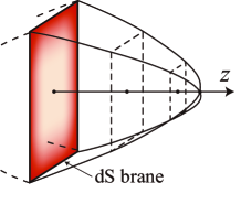
(a) RS model with de Sitter brane

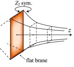
(b) RS-II model

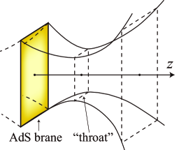
(c) KR model

Figure 2: Schematic of (a) the RS model with de Sitter brane, (b) the RS-II model and (c) the KR model in the Poincaré coordinates.

2.4 DGP model

The DGP model provides another way to localize four-dimensional graviton onto the brane [7]. The brane in this model has its own four-dimensional Einstein-Hilbert action, which may be induced by e.g. quantum correction of matter fields on the brane [26]. The original DGP model is composed of four-dimensional brane in the bulk without a higher-dimensional cosmological constant, and its full action is given by

$$S_{\text{DGP}}=-\frac{1}{16\pi G_{5}}\int d^{5}x\sqrt{-g}\,R_{\text{5D}}-\int d^{4}x\sqrt{-\gamma}\left(\frac{1}{16\pi G_{4}}R_{\text{4D}}+L_{\text{matter}}\right)~{}.$$ (26)

The unperturbed background is simply given by five-dimensional Minkowski space bounded on one side by a four-dimensional $Z_{2}$-symmetric Minkowski brane.

The basic feature of gravity on the brane in this model can be understood by investigating an analogous five-dimensional scalar field toy model whose equation of motion is given by

$$\left[G_{5}^{-1}\Box+\delta(y)G_{4}^{-1}\Box^{(4)}\right]\phi=\delta(y)J,$$ (27)

where $J$ is the source term localized on the brane. $y$ is the coordinate in the direction of the extra dimension, and the brane is located at $y=0$. Using the Fourier components with respect to four-dimensional coordinates, which are expressed by associating a tilde “$~{}\tilde{}~{}$”, the equation becomes $G_{5}^{-1}(p^{2}-\partial_{y}^{2})\tilde{\phi}+\delta(y)G_{4}^{-1}p^{2}\tilde{\phi}=-\delta(y)\tilde{J}$, where $p$ is the four-dimensional momentum parallel to the brane. Integrating the above equation over an infinitesimal distance across the brane, we obtain $-2G_{5}^{-1}\partial_{y}\tilde{\phi}+G_{4}^{-1}p^{2}\tilde{\phi}=-\tilde{J}.$ The solution in the bulk that is normalizable is given by $\tilde{\phi}=\tilde{\phi}_{0}e^{-p|y|}$. Substituting this into the above equation, we obtain $\left[2G_{5}^{-1}p+G_{4}^{-1}p^{2}\right]\tilde{\phi}=-\tilde{J}.$ Hence, the propagator behaves like

$$\tilde{G}(p)\sim\frac{1}{p^{2}+r_{c}^{-1}p}~{},$$ (28)

where $r_{c}\equiv G_{5}/2G_{4}$ defines the crossover scale for this propagator: the propagator reduces to an ordinary four-dimensional one in a short distance scale $p^{-1}\ll r_{c}$ while it becomes a five-dimensional one in a long distance scale $p^{-1}\gg r_{c}$.

The graviton propagator in this model has a structure similar to Eq. (28), and then the behavior of gravity is modified in a long distance scale while the four-dimensional gravity is kept intact in a short distance scale in this model. This peculiar property of the model brings about many interesting phenomena such as the self-accelerating cosmology [27, 28, 29], and further motivated some other cosmological models [30]. Many studies on the DGP cosmology showed that the self-accelerating branch of solutions suffers from the presence of a ghost excitation [31, 32, 33, 34, 35, 36]. Here a ghost means a degree of freedom whose kinetic term has an opposite sign, and it leads to pair production instability in quantum theory. However, there are also some arguments that this ghost might be less harmful compared with the other ghosts [37, 38].

The DGP model is closely related to massive gravity theories [7, 39, 40, 41, 42]. At the linear level, a four-dimensional ghost-free massive gravity theory can be defined by

$$S_{m}=\frac{1}{16\pi G_{4}}\int d^{4}x\sqrt{-g}\biggl{[}R+\frac{m_{g}^{2}}{4}\left(h^{\mu\nu}h_{\mu\nu}-h^{2}\right)\biggr{]}~{},$$ (29)

where $m_{g}$ is the graviton mass and $h_{\mu\nu}\equiv g_{\mu\nu}-g^{(0)}_{\mu\nu}$ is the metric perturbation from the background metric $g^{(0)}_{\mu\nu}$. The quadratic effective action in the DGP model has a structure similar to this one with $m_{g}\sim\sqrt{p/r_{c}}$, and thus it shares many properties with a massive gravity theory. In this regard, the DGP model may be viewed as a covariant non-linear completion of a massive gravity theory.

In the massive gravity theory defined by Eq. (29), non-zero graviton mass alters the gravitational attraction to be a short-ranged one. A perturbative analysis shows that the Newton potential in this theory is given by $V\propto e^{-m_{g}r}/r$. More striking effect of the graviton mass in linear perturbation is the discontinuity in the spatial component of metric perturbation from Minkowski background, which is so-called van Dam-Veltman-Zakharov (vDVZ) discontinuity [43, 44, 45]. Because of this discontinuity, even if we take the massless limit, the light bending around a star is predicted to be 25% less compared with the Einstein gravity. The perturbative analysis, however, is known to break down on a short distance scale [46]. By solving the Einstein equation to sub-leading order, one finds that next-to-leading order correction with respect to $r_{g}$ is given by $\mathcal{O}\left(r_{g}/m_{g}^{4}r^{5}\right)$, where $r_{g}$ is the Schwarzschild radius of the matter source. Thus, the perturbative expansion with respect to $r_{g}$ breaks down for $r\lesssim r_{*}\equiv\left(r_{g}/m_{g}^{4}\right)^{1/5}$. This critical length scale $r_{*}$ is called the Vainshtein scale. The perturbative solution will be correct for $r\gg r_{*}$, but the non-linearity plays an important role on short distance scales $r\lesssim r_{*}$. The vDVZ discontinuity is thought to be resolved by the effect of non-linearity, which is called Vainshtein mechanism.

In the DGP model, the graviton mass is roughly given by $m_{g}\sim\sqrt{1/r_{c}r}$, and then the Vainshtein scale becomes $r_{*}\sim\left(r_{g}r_{c}^{2}\right)^{1/3}$. Note that the hierarchy of the length scales becomes $r_{g}\ll r_{*}\ll r_{c}$ for an ordinary astrophysical object. The gravitational field for $r\gg r_{*}$ is well approximated by a linear theory, and non-linearity must be taken into account for $r\lesssim r_{*}$. In Refs. Gruzinov and TanakaDGP, systematic perturbative expansion which has smooth massless limit $m_{g}\to 0$ was developed. As a result, it was found to be important to solve the Einstein equations partly up to second order on a short distance scale $r\lesssim r_{*}$.

3 Holographic interpretation of the warped compactification

3.1 Effective Einstein equations on the brane

Before we discuss the holographic view of RS-II and KR models based on the AdS/CFT correspondence, let us study the effective four-dimensional Einstein equations on the brane in these models [49]. As we briefly mentioned in §2.2, a brane is characterized by its unit normal $s_{M}$ and the induced metric defined as $\gamma_{MN}\equiv g_{MN}-s_{M}s_{N}$. We take the convention that the normal $s^{M}$ points in the direction toward the bulk spacetime from the brane. Another quantity that specifies the geometry of the brane is the extrinsic curvature, defined by $K_{\mu\nu}\equiv-\gamma_{\mu}^{~{}M}\gamma_{\nu}^{~{}N}{\rm NewA}_{M}s_{N}$, which describes how the brane is embedded in the bulk spacetime.

The effective Einstein equations on the brane is obtained by projecting the five-dimensional equations onto the brane and to the normal. The key equations for this reduction are the Gauss-Codazzi formula and other formulae for the projection,

$$\gamma_{\mu}^{~{}M}\gamma_{\nu}^{~{}N}\gamma_{P}^{~{}\rho}\gamma_{\lambda}^{~{}Q}R^{P}_{~{}MNQ} =\overset{\text{\tiny$(\gamma)$}}{R}{}^{\rho}_{~{}\lambda\mu\nu}-K^{\rho}_{~{}\mu}K_{\nu\lambda}+K^{\rho}_{~{}\nu}K_{\mu\lambda}~{},$$ (30)

$$s^{M}\gamma_{\mu}^{~{}N}R_{MN} =D_{\mu}K-D_{\nu}K^{\nu}_{~{}\mu}~{},$$ (31)

$$\gamma_{\mu M}s^{P}\gamma_{\nu}^{~{}N}s^{Q}R^{M}_{~{}PNQ} =\pounds_{s}K_{\mu\nu}+K_{\mu\rho}K^{\rho}_{~{}\nu}~{},$$ (32)

where $\overset{\text{\tiny$(\gamma)$}}{R}_{\mu\nu}$ and $D_{\mu}$ are the four-dimensional Ricci tensor and the covariant derivative with respect to $\gamma_{\mu\nu}$, and $\pounds_{s}$ is the Lie derivative with respect to $s_{M}$. Projecting the defining equation of the Weyl tensor

$$C_{MPNQ}\equiv R_{MPNQ}-\frac{2}{3}\left(g_{M[N}R_{Q]P}-g_{P[N}R_{Q]M}\right)+\frac{1}{6}g_{M[N}g_{Q]P}R~{},$$ (33)

into the directions parallel to the brane, and contracting two indices, one can derive an expression for the projected five-dimensional Einstein tensor with the aid of Eq. (30) as

$$\overset{\text{\tiny$(\gamma)$}}{R}_{\mu\nu}-\frac{1}{2}\overset{\text{\tiny$(\gamma)$}}{R}\gamma_{\mu\nu} =\frac{16\pi G_{5}}{3}\left\{\gamma_{\mu}^{~{}M}\gamma_{\nu}^{~{}N}\mathcal{T}_{MN}+\left(s^{M}s^{N}\mathcal{T}_{MN}-\frac{1}{4}\mathcal{T}^{M}_{~{}M}\right)\gamma_{\mu\nu}\right\}$$

$$\phantom{=}\;+KK_{\mu\nu}-K_{\mu}^{~{}\rho}K_{\nu\rho}-\frac{1}{2}\left(K^{2}-K^{\rho\lambda}K_{\rho\lambda}\right)\gamma_{\mu\nu}-E_{\mu\nu}~{},$$ (34)

where we used the five-dimensional Einstein equation

$$R_{MN}-\frac{1}{2}Rg_{MN}=8\pi G_{5}T_{MN}~{},\qquad\mathcal{T}_{MN}\equiv\frac{-\Lambda_{\text{5D}}}{8\pi G_{5}}g_{MN}+\left(-\lambda\gamma_{MN}+\tau_{MN}\right)\delta(y)~{},$$ (35)

in which $\lambda$ and $\tau_{MN}$ are the brane tension and the energy-momentum tensor confined on the brane, as before. The coordinate $y$ in the delta function here is that of the Gaussian-normal coordinates with respect to the brane, in which the five-dimensional metric is expressed as

$$ds^{2}=dy^{2}+\gamma_{\mu\nu}dx^{\mu}dx^{\nu}~{}.$$ (36)

(Here, for notational simplicity, we do not put a bar “$~{}\bar{}~{}$” to the quantities in the Gaussian-normal coordinates.) A projection of the five-dimensional Weyl tensor $E_{\mu\nu}$ in Eq. (34) is defined by

$$E_{\mu\nu} \equiv C^{M}_{~{}NPQ}\,s_{M}\gamma_{\mu}^{~{}N}s^{P}\gamma_{\nu}^{~{}Q}~{}.$$ (37)

To derive the junction condition at the brane, let us rewrite the left-hand side of Eq. (34) using Eqs. (30) and (32) as

$$\overset{\text{\tiny$(\gamma)$}}{R}_{\mu\nu}-\frac{1}{2}\overset{\text{\tiny$(\gamma)$}}{R}\gamma_{\mu\nu} =\gamma_{\mu}^{~{}M}\gamma_{\nu}^{~{}N}\left(R_{MN}-\frac{1}{2}Rg_{MN}\right)+KK_{\mu\nu}-K_{\mu\rho}K^{\rho}_{~{}\nu}-\pounds_{s}K_{\mu\nu}$$

$$\phantom{=}\;+\frac{1}{2}\left(-K^{2}+2\pounds_{s}K-K_{\rho\lambda}K^{\rho\lambda}\right)\gamma_{\mu\nu}~{}.$$ (38)

In the Gaussian-normal coordinates (36), the Lie derivative $\pounds_{n}$ reduces to a simple coordinate derivative $\partial_{y}$. The terms other than this Lie derivative and the delta function concealed in the five-dimensional Einstein tensor are all regular on the brane. Then, integrating Eq. (38) along $y$ over an infinitesimal domain $y\in(-\epsilon,\epsilon)$, we recover Eq. (9). This equation is called the Junction conditions for the bulk metric [50].

Since $Z_{2}$-symmetry across the brane demands $\lim_{y\to+0}K_{\mu\nu}=-\lim_{y\to-0}K_{\mu\nu}$, we find that the junction conditions (9) reduce to

$$K_{\mu\nu}-K\gamma_{\mu\nu}=4\pi G_{5}\left(-\lambda\gamma_{\mu\nu}+\tau_{\mu\nu}\right)~{},$$ (39)

where $K_{\mu\nu}$ is understood as $\lim_{y\to+0}K_{\mu\nu}$. Using this formula, we can transform Eq. (34) further into

$$\overset{\text{\tiny$(\gamma)$}}{R}_{\mu\nu}-\frac{1}{2}\overset{\text{\tiny$(\gamma)$}}{R}\gamma_{\mu\nu}=-\Lambda_{\text{4D}}\gamma_{\mu\nu}+8\pi G_{4}\tau_{\mu\nu}+\left(8\pi G_{5}\right)^{2}\pi_{\mu\nu}-E_{\mu\nu}~{},$$ (40)

where the four-dimensional cosmological constant and the Newton constant are given by

$$\Lambda_{\text{4D}}=\frac{1}{2}\left(\Lambda_{\text{5D}}+\frac{\left(8\pi G_{5}\right)^{4}}{6}\lambda^{2}\right)~{},\qquad G_{4}=\frac{4\pi G_{5}\lambda}{3}~{},$$ (41)

and

$$\pi_{\mu\nu}\equiv-\frac{1}{4}\tau_{\mu\rho}\tau_{~{}\nu}^{\rho}+\frac{1}{12}\tau\tau_{\mu\nu}+\frac{1}{8}\tau_{\rho\lambda}\tau^{\rho\lambda}\gamma_{\mu\nu}-\frac{1}{24}\tau^{2}\gamma_{\mu\nu}$$ (42)

is the contribution quadratic in $\tau_{\mu\nu}$. As we can see in Eq. (40), a brane observer sees an effective energy-momentum tensor $\left(6G_{5}\right/\lambda)\pi_{\mu\nu}-(8\pi G_{4})^{-1}E_{\mu\nu}$. Since $E_{\mu\nu}$ is traceless by its construction, and the trace part coming from $\pi_{\mu\nu}$ term can be identified with the trace anomaly [51], this effective energy-momentum tensor may be regarded as the contribution from some conformal fields, which we will discuss in the next section. References Kanno:2002iaa and McFadden:2004se constructed the effective action on the brane that derives Eq. (40), and argued their relationship with the AdS/CFT correspondence (for a review see Ref. Soda:2010si).

The effective Einstein equations on the brane in the DGP model was studied in Ref. MizunoDGP in detail. The DGP model can be seen as a variant of the RS model with exotic matter whose Lagrangian is the four-dimensional Ricci scalar. Then, the modification to the effective Einstein equation only appears in the brane energy-momentum tensor. For the DGP model, whose brane-localized part of the Lagrangian is

$$L_{\text{brane}}=\frac{1}{16\pi G_{4}}R_{\text{4D}}-\lambda+L_{\text{matter}}~{},$$ (43)

the energy-momentum tensor on the brane is given by

$$\tau_{\mu\nu}=-2\frac{\delta L_{\text{brane}}}{\delta\gamma^{\mu\nu}}+\gamma_{\mu\nu}L_{\text{brane}}=-\lambda\gamma_{\mu\nu}+T^{\text{matter}}_{\mu\nu}-\frac{1}{8\pi G_{4}}G^{\text{4D}}_{\mu\nu}~{}.$$ (44)

We will immediately obtain the effective Einstein equations for the DGP model by plugging this $\tau_{\mu\nu}$ into Eq. (40) with the bulk cosmological constant being set to zero. In Ref. MizunoDGP, this effective equations were used to study various settings in the DGP model.

3.2 AdS/CFT correspondence in the RS-II braneworld model

In the preceding sections, we introduced the braneworld models that have the AdS spacetime as the unperturbed bulk spacetime, and surveyed basic properties of gravity in these models. In this subsection, we focus on another aspect of these models, which is the non-trivial correspondence between the classical gravity in higher dimensions and the gauge theory on the brane suggested from the AdS/CFT correspondence.

In the RS-II model, the brane serves as a boundary of the asymptotically AdS bulk. Then, naively thinking, it might be possible to apply to this model the AdS/CFT correspondence, which implies the correspondence between the classical supergravity and the conformal field theory on the AdS boundary [8, 9, 56, 57, 58, 59]. Such a proposition was firstly made by Refs. WittenComment and VerlindeComment, and made more concrete in Refs. Gubser,HR,Savonije:2001nd.

We review below the discussion of Ref. HR about the relationship between the RS model and the CFT on the brane. The AdS/CFT correspondence states that the supergravity partition function, $Z[\bm{\gamma}]$, is related to the generating functional of connected Green’s functions for the CFT on the boundary geometry, $W_{\text{CFT}}[\bm{\gamma}]$, as

$$Z[\bm{\gamma}]=\int d[\bm{g}]\exp\left(iS_{\text{grav}}[\bm{g}]\right)=\int d[\phi]\exp\left(iS_{\text{CFT}}[\phi;\bm{\gamma}]\right)\equiv\exp\left(iW_{\text{CFT}}[\bm{\gamma}]\right)~{},$$ (45)

where $\gamma_{\mu\nu}$ is the conformally-rescaled boundary metric and $\phi$ symbolically represents the fields contained in the CFT. The supergravity action for the bulk spacetime, $S_{\text{grav}}$, is given by

$$S_{\text{grav}}=S_{\text{EH}}+S_{GH}+S_{1}+S_{2}+S_{3}~{},$$ (46)

where

$$S_{\text{EH}}=\frac{1}{16\pi G_{5}}\int d^{5}x\sqrt{-g}\left(R+2\Lambda\right)~{},\quad S_{\text{GH}}=\frac{1}{8\pi G_{5}}\int d^{4}x\sqrt{-\gamma}K$$ (47)

are respectively the Einstein-Hilbert action for the bulk gravity and the Gibbons-Hawking boundary term introduced to make the variational problem to be well-defined [63]. When we move the boundary toward the AdS boundary, this $S_{\text{EH}}$ diverges since the volume of an AdS spacetime is infinite. To regularize it, the counter terms, $S_{1},S_{2}$ and $S_{3}$, are introduced to the gravitational action (46). To be more precise, let us consider the asymptotic AdS metric

$$ds^{2}={\ell^{2}\over z^{2}}\left(\gamma_{\mu\nu}dx^{\mu}dx^{\nu}+dz^{2}\right)~{}.$$ (48)

First, we cut the region with $z<\epsilon\ll\ell$ from this spacetime. Next, we expand the gravitational action in terms of the small parameter $\epsilon$. Then, we obtain some terms that diverge in the limit of $\epsilon\to 0$. The negatives of such terms are given by

$$S_{1}=\frac{-3}{8\pi G_{5}\ell}\int d^{4}x\sqrt{-\gamma}~{},\quad S_{2}=\frac{-\ell}{32\pi G_{5}}\int d^{4}x\sqrt{-\gamma}\overset{\text{\tiny$(\gamma)$}}{R}~{},$$

$$S_{3}=\frac{-\ell^{3}\log\epsilon}{64\pi G_{5}}\int d^{4}x\sqrt{-\gamma}\left(\overset{\text{\tiny$(\gamma)$}}{R}_{\mu\nu}\overset{\text{\tiny$(\gamma)$}}{R}{}^{\mu\nu}-\frac{1}{3}\overset{\text{\tiny$(\gamma)$}}{R}{}^{2}\right)~{},$$ (49)

and are identified with the counter terms.

Now, let us consider the RS-II model, whose action is in the current notation given by

$$S_{\text{RS}}=S_{\text{EH}}+S_{\text{GH}}+2S_{1}+S_{m}~{},$$ (50)

where $S_{m}$ is the action of the matter confined on the brane. $2S_{1}$ is precisely corresponding to the action for the brane tension $3/4\pi G_{5}\ell$. Let us construct the partition function from this $S_{\text{RS}}$. It is given as

$$Z[\bm{\gamma}] =\int d[\delta\bm{g}]d[\phi]\exp\left(iS_{\text{RS}}[\bm{g}_{0}+\delta\bm{g}]\right)$$

$$=\exp(2iS_{1}[\bm{\gamma}_{0}+\bm{\gamma}])$$

$$\phantom{=}\;\;\times\int d[\delta\bm{g}]d[\phi]\exp\left(iS_{\text{EH}}[\bm{g}_{0}+\delta\bm{g}]+iS_{\text{GH}}[\bm{g}_{0}+\delta\bm{g}]+iS_{m}[\phi;\bm{\gamma}_{0}+\bm{\gamma}]\right)$$

$$=\exp(2iS_{1}[\bm{\gamma}_{0}+\bm{\gamma}])\left(\int_{\text{\hbox to0.0pt{one-bulk\hss}}}\;d[\delta\bm{g}]d[\phi]\exp\left(iS_{\text{EH}}[\bm{g}_{0}+\delta\bm{g}]+iS_{\text{GH}}[\bm{g}_{0}+\delta\bm{g}]\right)\right)^{2}$$

$$\phantom{=}\;\;\times\int d[\phi]\exp\left(iS_{m}[\phi;\bm{\gamma}_{0}+\bm{\gamma}]\right)~{},$$ (51)

where in the third equality we used the fact that the RS-II model has two bulk regions which are related by $Z_{2}$-symmetry with each other. Now, we apply Eq. (45) of the AdS/CFT correspondence, which holds for the regularized gravitational action (46), to this equation. Firstly, Eqs. (45) and (46) imply

$$\int_{\text{\hbox to0.0pt{one-bulk\hss}}}~{}d[\delta\bm{g}]d[\phi]\exp\left(iS_{\text{EH}}+iS_{\text{GH}}\right)[\bm{g}_{0}+\delta\bm{g}] =\exp\left(iW_{\text{CFT}}-iS_{1}-iS_{2}-iS_{3}\right)[\bm{\gamma}_{0}+\delta\bm{\gamma}]~{}.$$ (52)

Plugging this into Eq. (51), we obtain

$$Z[\bm{\gamma}]=\exp\left(2iW_{\text{CFT}}-2iS_{2}-2iS_{3}\right)[\bm{\gamma}_{0}+\delta\bm{\gamma}]\int d[\phi]\exp\left(iS_{m}[\phi;\bm{\gamma}_{0}+\bm{\gamma}]\right)~{}.$$ (53)

Remarkably, $-2S_{2}$ is equal to the four-dimensional Einstein-Hilbert action. Thus, the system described by the partition function on the right-hand side is that of the four-dimensional CFT interacting with the four-dimensional gravity and the matter described by $-2S_{2}$ and $S_{m}$, respectively. The other term, $S_{3}$, is the higher-curvature correction to the theory, and it represents the renormalization scale dependence of the cutoff CFT.

This correspondence in the RS-II model is an extension of the original AdS/CFT correspondence in the sense that the former reduces to the latter in the limit of $\epsilon\to 0$. Namely, the correspondence in the RS-II model is different from the original one in that the boundary is not sent to the AdS boundary but is determined by the brane position. The position of the boundary in the bulk corresponds to the UV cutoff energy scale of the CFT. When we measure the energy scale by the proper length on the brane, where the warp factor is usually normalized to unity, the UV cutoff energy scale is $\sim\ell^{-1}$. If we send the brane to the AdS boundary, the cut-off energy scale becomes higher. However, this shift of the location of the brane can be absorbed by the overall re-normalization of the warp factor. Therefore, sending the boundary to the AdS boundary is equivalent to observe phenomena in the IR limit. Hence, we expect that this extended correspondence should hold at least for deep IR phenomena compared with the bulk curvature scale.

3.3 Supporting evidence for the correspondence

Although there is no proof of this extended correspondence in the RS-II model, there are many pieces of supporting evidence. We show some examples of them below.

• Garriga and Sasaki[64] considered a bulk black hole in the expanding braneworld. The presence of a bulk black hole naturally induces additional thermal radiation of CFT to the boundary effective theory. When the temperature is well below the AdS scale, the entropy of this radiation agrees with the entropy determined from the area of the black hole in the AdS bulk.

• Duff and Liu [65] calculated weakly coupled CFT’s one-loop correction to the graviton propagator, and found that the Newton potential acquires a correction suppressed by a factor of $\mathcal{O}(\ell^{2}/r^{2})$. This correction including its coefficient agrees with that in the RS-II model, Eq. (19), which is caused by five-dimensional gravity in the bulk [15]. This coincidence between four and five-dimensional description was reconfirmed by Anderson et al.[66, 67] using vacuum polarization of various fields around a Schwarzschild black hole.

• Shiromizu et al.[51] studied the relationship between CFT energy-momentum tensor in the four-dimensional point of view and effective energy-momentum tensor on the brane in the five-dimensional point of view. As a result, the CFT’s trace anomaly was found to be reproduced in the five-dimensional point of view from the $\pi_{\mu\nu}$ term in the effective Einstein equations, Eq. (42), as $\left<T^{\mu}_{~{}\mu}\right>_{\text{CFT}}=\ell\pi^{\mu}_{~{}\mu}/4$.

• Tanaka[68] studied the Friedmann-Lemaitre-Robertson-Walker cosmology realized on the braneworld model. It was shown that the effective equations of motion for four-dimensional tensor perturbation on the brane, which is obtained in the five-dimensional classical gravity picture, agree with those derived in the four-dimensional CFT picture.

• Grisa and Pujolàs[69] constructed solutions of three-dimensional domain wall localized on the four-dimensional brane in the RS-II model to use it as a testbed of the correspondence. In the four-dimensional point of view, the domain wall tension is renormalized due to the CFT’s trace anomaly. They found that this renormalization of tension is reproduced in the five-dimensional point of view as an effect of brane acceleration in the five-dimensional bulk.

We also have interesting observations, although they are not the evidence directly supporting the argument that five-dimensional gravity phenomena is described by four-dimensional general relativity with CFT corrections. Let us consider four-dimensional de Sitter spacetime. This de Sitter spacetime is associated with finite temperature due to existence of cosmological horizon. Das et al.[70] considered the RS model with de Sitter brane, and argued that this de Sitter temperature on the brane can be reproduced in the five-dimensional point of view from accelerating motion of the brane in the bulk. Iwasita et al.[25] also studied this model, and showed that the holographic entanglement entropy in the five-dimensional picture coincides with the four-dimensional de Sitter entropy calculated from the cosmological horizon area or from the Euclidean path integral.

Assuming the correspondence to be correct, some attempts to give predictions about the cosmology realized on the RS model were made. Reference HR applied the correspondence to inflating universe and quantum fluctuation of strongly-coupled large $N$ CFT therein. They constructed an effective action of the CFT applying the correspondence to the RS model with de Sitter brane. An advantage of this approach is that the effect of full quantum effect of the matter fields, which is usually out of reach of perturbative approaches, can be taken into account. From the effective action, they showed that the tensor perturbation due to the quantum effect is highly suppressed in short scale. Since any matter field can be expected to behave like CFT in high energy scale, such a prediction may apply to general matter fields which are strongly coupled in such regime.

An upper bound on $\ell$ was given from the production of CFT particles in Ref. Gubser assuming the correspondence to hold, and this bound was re-analyzed later by Ref. Hebecker:2001nv more explicitly based on the five-dimensional gravity picture. They considered scattering of standard model particles and CFT in the Friedmann universe. In the five-dimensional gravity picture, the corresponding process is the bulk graviton emission from the radiation on the Freedman-Robertson-Walker brane. When the center-of-mass energy of the standard model particles $\sqrt{s}$ is much higher than the AdS bulk energy scale $1/\ell$, those particles will feel the five-dimensional gravity. Thus, its cross section to emit the bulk graviton will be proportional to $G_{5}$, and we may expect the cross section to be $\sigma(s)\sim G_{5}\sqrt{s}$ from the dimensional analysis. Multiplying the effective number of the brane matter’s degrees of freedom, we obtain the total cross section. From this cross section, taking into account the redshift factor properly, one can estimate the energy leakage to the bulk graviton. This bulk graviton will be seen by a brane observer as “dark radiation” which interacts only gravitationally with other particles. The dark radiation density $\rho_{d}$, which turns out to depend logarithmically on the maximum temperature of the universe, has to be smaller than the bound from the nucleosynthesis. This bound marginally accepts $\ell\approx 1\,\text{mm}$ even if the maximum temperature of the universe is as high as the fundamental energy scale $M_{5}$. They showed that this energy leakage into the bulk graviton can be equivalently viewed as the leakage into the large $N$ CFT, and also pointed out that cosmological implications at high energy scale may depend on microscopic definition of the correspondence, i.e., the background spacetime, such as AdS₅ or AdS${}_{5}\times S^{5}$, on which we consider the model (see also Ref. ArkaniHamed:2000ds).

3.4 Holography in the KR model

Since the KR model can be obtained as a continuous deformation of the RS-II model, it is natural to expect that the bulk/brane correspondence persists even in the KR model. Such a view was already taken in the original paper of the KR model [16] and has been investigated in many ways. For example, the “almost zero mode” in the KR model we mentioned in §2.3 was reproduced in four-dimensional point of view as a graviton dressed with one-loop correction of the CFT [73, 74, 75, 76]. This issue is also pursued in Ref. insidestory, and they interpreted the running of the effective four-dimensional Planck mass, $M_{\text{4D}}^{2}\propto 1+\mathcal{O}(1)\left(\frac{\ell}{L}\right)^{2}\frac{\mathcal{R}}{L}$, as renormalization group flow driven by quantum effects of the CFT. In Refs. KRstring_orig,KRstring,DeWolfe,DeWolfe2, the realization of the KR model within the string theory and the AdS/CFT correspondence in such a system with defects on the AdS boundary are discussed.

Figure 3: A schematic picture of the a conformally transformed section of the KR model sliced at a time constant surface. The brane touches the AdS boundary, forming a $S^{2}$ boundary between them. CFT₁ is living on the brane while CFT₂ on the AdS boundary.

In the KR model with a single brane, there are two boundaries surrounding the bulk: the brane and the half of the AdS boundary as depicted in Fig. 3. Then, the bulk gravity will induce one set of CFT on each boundary and there will be two sets of CFT in total. Naively thinking, each CFT would have distinct bulk region which is dual to it. In Ref. BR, such an idea was pursued by considering causal structure of the bulk spacetime. As a result of this study, it was realized that the “holographic domains” of the bulk, which are the bulk regions corresponding to the respective CFTs on the boundaries, are given by the bulk regions divided at the “throat” of the bulk at which the warp factor is minimized. Since gravitational waves can freely pass through this throat in the five-dimensional description, it is expected in the four-dimensional picture that the CFTs on the brane and the AdS boundary communicate each other through the common $S^{2}$ boundary. This transparent boundary condition at the common boundary is found to be essential to reproduce the graviton mass by evaluating the correction coming from the CFT loop [73, 74].

4 Black holes in ADD model: Kaluza-Klein black holes

In this and the subsequent sections, we discuss black hole solutions in the braneworld models. Let us begin with the ADD model, which is the simplest braneworld model. Since the brane in the ADD model does not have tension, the black objects in this model are almost equivalent to those in a Kaluza-Klein compactified spacetime. The properties of such black objects have been studied intensively and summarized in reviews such as Refs. Kol and Harmark_review. In this section, we only summarize some points important for discussions in the following sections, and also we pick up some topics that is not discussed in the above reviews.

4.1 Black holes escaping into the bulk

One of the interesting predictions of braneworld models with its fundamental gravity scale at TeV is that small black holes can be created in high energy collisions of particles at energy scale within the reach of forthcoming experiments [80]. When two particles on a brane collide at a center of mass energy larger than the fundamental gravity scale with sufficiently small impact parameter, the system will form a black hole. The black hole formed in this process is small compared with the size of extra dimensions in the context of the ADD braneworld. Therefore the role of the brane and the finiteness of the bulk is not relevant in most respects. Properties of such black holes smaller than extra dimension size are summarized in references such as Ref. Kanti:2004nr. Here we just mention an aspect which is peculiar to the braneworld setup: escaping black holes from the brane.

After its formation, the black hole will start to emit Hawking radiation partly into higher-dimensional bulk modes [82]. The emission of higher-dimensional modes will cause the recoil of the black hole into the extra dimensions unless the process is prohibited by symmetry, e.g., $Z_{2}$-symmetry in codimension-one case. The interaction between a small black hole and a brane when the black hole is kicked relative to the brane was first studied in Refs. art1 and art1-b. It was pointed out that the black hole can escape from the brane due to emission of higher-dimensional modes, using a field theory model in which such a black hole is described as a massive scalar particle with internal degrees of freedom. If the black hole leaves the brane, Hawking radiation into the brane modes suddenly terminates and it will leave a distinctive experimental signature. In Ref. art2 the same problem was studied by investigating the dynamics of Nambu-Goto branes in black hole spacetimes. This is to be called the probe-brane approximation, in the sense that the tension of the brane is assumed to be negligibly small. The results of Ref. art2 confirmed the basic claim in Ref. art1, further suggesting that the escape of the black hole occurs through reconnection of the brane. A small piece of the brane attached to the black hole is pinched off from the main body of the brane. In Ref. art3, these results were confirmed also in a model in which the brane is described by a domain wall composed of a scalar field. In Ref. Flachi:2006ev, the critical escape velocity was derived by studying the interaction between a Nambu-Goto brane and a black hole assuming adiabatic (quasi-static) evolution. It was found that, to lowest order effects in the tension, the critical escape velocity does not exist for codimension-one branes, while it does for higher codimension branes. These results can be qualitatively understood by considering the gravitational force caused by a light brane on a flat background spacetime perturbatively. A codimension-one brane produces repulsive force while a brane with codimensions higher than 2 makes attractive force. Codimension-two branes are neutral in this test particle approximation as in the well-known case of cosmic strings in four dimensions, but finite amount of initial velocity is required to escape when treated in the opposite limit, i.e., in the test brane approximation.

4.2 Solution sequences of KK black objects

We consider below the black objects in a KK-compactified spacetime which is asymptotically $\mathcal{M}^{d}\times S^{1}$, where $\mathcal{M}^{d}$ is $d$-dimensional Minkowski spacetime. There are typically two types of black objects in this model: a black string wrapping the bulk and a black hole localized in the bulk. These solutions can be parametrized by its mass and length along the KK direction at infinity.

Properties of localized black holes for $d=3$ was studied, e.g., in Refs. Bogojevic:1990hv,Korotkin:1994dw,Frolov:2003kd. For $d\geq 4$, numerical solutions have been constructed in, e.g., Refs. Kol:2003if,Sorkin,Kudoh:2003ki,KudohBS. As for analytical approaches, perturbative solutions were constructed by Refs. Gorbonos:2004uc and Karasik:2004ds using the matched asymptotic expansion technique, and by Ref. Harmark:2003yz using special coordinates which interpolate spherical coordinates near the black hole and cylindrical coordinates at infinity [98].

We also have a black string as another black object in KK spacetime. In the present setup, black string solutions are given by

$$ds^{2}=dy^{2}+\gamma_{\mu\nu}dx^{\mu}dx^{\nu},$$ (54)

where $y$ is the coordinate in the direction of $S^{1}$ and $\gamma_{\mu\nu}$ is any black hole solution of the $d$-dimensional vacuum Einstein equations. This solution suffers from instability when, roughly speaking, the size of the horizon radius becomes smaller than the length of $S^{1}$. This instability is called the Gregory-Laflamme instability [99, 100]. A marginally unstable mode arises when the parameters in the solutions are tuned to the critical values. Existence of such a marginally unstable mode indicates the appearance of a new branch of solutions. Namely, a solution perturbed in the direction of the marginally unstable mode will also be a static solution, and the sequence of solutions will continue to exist to the non-linear level. The solutions in this new branch will be non-uniform static black strings in this case. The properties of this non-uniform string was studied from both analytical side [101, 102, 103] and numerical side [103, 104, 105]. It was found that, as long as $d\leq 13$, this non-uniform black string has larger mass compared to a uniform black string with the same entropy, and then it cannot be an endpoint of the Gregory-Laflamme instability in a micro-canonical ensemble.

The first construction of numerical solutions was done in the following way by Wiseman [103], based on the numerical technique developed in Ref. Wiseman:2001xt. A static metric in axisymmetric five-dimensional spacetime can be expressed without loss of generality as

$$ds^{2}=\frac{\ell^{2}}{z^{2}}\Bigl{(}-T^{2}dt^{2}+e^{2R}\left(dr^{2}+dz^{2}\right)+r^{2}e^{2C}d\Omega^{2}\Bigr{)}~{},$$ (55)

where $r$ and $z$ are the radial coordinate along the brane and the one in the direction of the extra dimension, respectively. An advantage of this metric form is that the two-dimensional part spanned by $r$ and $z$ is only specified to be conformally flat, and then we may set the locations of both the brane and the horizon to be constant coordinate surfaces by applying conformal transformation. The Einstein equations become elliptic partial differential equations for free functions $T$, $R$ and $C$, and one can solve them with appropriate boundary conditions at the brane, axisymmetric axis and asymptotic boundary. Solving them numerically by the relaxation method, solutions for non-uniform black strings were successfully constructed.

This non-uniform black string branch is thought to be connected to the localized black hole branch in the following manner. As we increase the deformation of a black string further, a cone-like structure develops where the radius of the black string shrinks to zero. After this cone-like structure formation, the sequence continues to the sequence with two isolated segments of the horizon, and this latter sequence corresponds to the localized black hole branch. Such a topology-changing transition in the solution sequence was proposed in Ref. Kol:2002xz. Incorporating this topology change, the phase diagram of black objects in KK-compactified spacetime would be as shown in Fig. 4. Now numbers of studies, such as Refs. Kudoh:2003ki and KudohBS which constructed numerical solutions about the entire solution branch, are supporting this phase diagram, although it is still difficult to resolve the transition numerically.

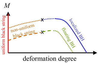
Figure 4: Solution sequences in the braneworld models with flat bulk. The horizontal axis denotes the deformation degree of the black object compared to a uniform black string. (this figure is taken from Ref. Tanaka:2009zz).

Another direction of study about black string in KK spacetime is to simulate its dynamical fate after the Gregory-Laflamme instability. Reference Horowitz:2001cz showed that it takes infinite affine time along the horizon for a black string to pinch off, assuming that any singularity is not formed on or outside the horizon. In Ref. Marolf:2005vn it was pointed out that such pinching off can occur in a finite asymptotic time if a singularity is formed on the horizon. The dynamical simulation of a deforming black string is pioneered by Refs. Choptuik:2003qd and Garfinkle:2004em, and recently a new result was reported which suggests that a black string shrinks to infinitesimal thickness leaving blob-like black holes [113]. The latter simulation also showed that this pinching process proceeds in a fractal manner, letting the string thinner and producing smaller black holes. They found that the time scale of this process is roughly proportional to local string radius, and then argued that a black string might pinch off in a finite asymptotic time.

When the extra dimension is not $S^{1}$ but $R^{2}$, the issue of finding a brane-localized black hole solution considerably simplifies since codimension-two objects with tension can be easily created by introducing deficit angle in an angular coordinate. A black hole solution localized on a codimension-two brane with tension are given just by introducing deficit angle to the higher-dimensional Schwarzschild solution [114].

5 Black holes in RS-II model

Our direct knowledge about black hole solutions in the RS-II model is quite limited. Hence, in §5.1, we first discuss the black hole solutions in the RS-II model applying the bulk/brane correspondence we introduced in §3. By doing so, we will obtain a prediction dubbed as the classical evaporation conjecture of the brane-localized black hole. We also discuss some connection to the black objects in the ADD model, and mention astrophysical constraints on the bulk curvature scale given by this conjecture. In §§5.2 and 5.3, we summarize studies on the black holes in the RS-II model and present supporting evidence for the conjecture. We focus on analytic approaches in §5.2 and numerical approaches in §5.3.

5.1 Holographic predictions

5.1.1 Classical evaporation conjecture of brane-localized BHs

If the duality in the RS-II model works even in the presence of a black hole, an interesting implication about its time evolution will be obtained as follows [115, 116]. Starting point of the argument is the properties of a four-dimensional black hole in the brane point of view. In the bulk/brane correspondence in the RS-II model, a large number of degrees of freedom of the quantum field theory (QFT) of $\mathcal{O}(\ell^{2}/G_{4})$ couple to the four-dimensional gravity. Such QFT degrees of freedom open a channel for the four-dimensional black hole to radiate its energy as the Hawking radiation very efficiently [117]. Then, that four-dimensional black hole will shrink and cannot remain static.

Since we are assuming the bulk/brane correspondence to hold, a five-dimensional counterpart of this shrinking four-dimensional black hole must exist. The point is that the bulk/brane correspondence indicates that this process should be described not by a quantum effect but by a classical dynamics in the five-dimensional picture, and the five-dimensional counterpart should be a classical black object in the bulk. Naively thinking, such a five-dimensional object will be a five-dimensional black hole localized on the brane, since it is a natural object to form as a consequence of a gravitational collapse on the brane. If so, according to the correspondence, the five-dimensional brane-localized black hole cannot be static and it will continuously reduce its area of the intersection with the brane as a result of classical dynamics.

We do not know much about such a dynamical process in five-dimensional classical gravity, but a warped black string solution gives us some implications. As mentioned earlier, the metric

$$ds^{2}=e^{-2|y-y_{+}|/\ell}\gamma_{\mu\nu}dx^{\mu}dx^{\nu}+dy^{2}~{},$$ (56)

is a solution in the RS-II model, if $\gamma_{\mu\nu}$ is a solution of four dimensional vacuum Einstein equations. When we take the Schwarzschild metric as $\gamma_{\mu\nu}$, we obtain a warped black string solution [118]. Although the induced metric on the brane is identical to the Schwarzschild black hole, this metric cannot be interpreted as the static final state formed after gravitational collapse on the brane because the solution is singular in the sense that the Kretschmann invariant increases indefinitely in the bulk. Moreover, the radius of the black string shrinks as we move away from the brane exponentially with the typical length scale $\ell$, although the length of the black string is infinitely long. Therefore it suffers from the Gregory-Laflamme instability [119] in the region where the horizon radius is smaller than $\mathcal{O}(\ell)$.

From this observation on a black string, one may expect that the brane-localized black hole will take a similar form to the black string chopped where the radius becomes $\mathcal{O}(\ell)$. Then, since the radius and the length of such a black object will be the same order at the tip, we may speculate that some instability similar to the Gregory-Laflamme instability continues to occur at the tip of this five-dimensional black hole. As a result of instability, a clump of horizon, almost pinched off from the main part of the horizon (see Fig. 5), will be formed. Then, the clump will fall into the bulk due to the acceleration $a=\left(\log\sqrt{-g_{tt}}\right)_{,y}\approx 1/\ell$ acting universally in the bulk in the direction from the brane to the bulk [120]. Such a deformation of the five-dimensional horizon in the bulk will decrease the four-dimensional intersection between the black hole and the brane, even though the total area of the five-dimensional black hole is not decreasing. As a result, an observer on the brane will see a four-dimensional black hole with diminishing area. This horizon deformation will be the five-dimensional counterpart of the four-dimensional black hole evaporation. This phenomenon is termed as classical evaporation of the brane black hole by Ref. tanaka.

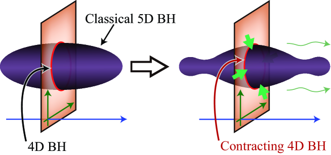
Figure 5: Schematic view of the conjectured “classical evaporation” process of a brane-localized black hole. The intersection of the five-dimensional black hole and the brane will be seen by a brane observer as a four-dimensional black hole with quantum correction. Decrease in the four-dimensional black hole area due to the Hawking radiation would be realized in the five-dimensional perspective by the deformation of the brane-localized black hole horizon into the bulk.

Some authors consider that the black string is one example of a static quantum corrected black hole [121]. As the induced metric on the brane is exactly identical to the four-dimensional Schwarzschild solution, there is no room for the QFT contribution to the energy-momentum tensor in this case. The authors of Ref. Fitzpatrick:2006cd claims that this feature is due to strong coupling of the CFT, that is, some confinement mechanism will emerge as a result of strong-coupling effect, and hence the number of effective QFT degrees of freedom around black holes will be not $\mathcal{O}(N^{2})$ but $\mathcal{O}(1)$. This reduction of degrees of freedom is assumed to be triggered by the curvature effects. Their idea is that the presence of small amount of curvature is sufficient to let most of QFT degrees of freedom inactive. If it is really the case, the effects of KK gravitons perturbatively derived on a conformally flat background, which includes the Friedmann universe, will be drastically changed once we take into account small gravitational wave perturbation. Then, many phenomena described as supporting evidence for the correspondence in §3.3 will show discontinuities between the cases on an exactly conformally flat background and on a slightly perturbed one from it, which we think quite unlikely.

There are also some other possibilities such as

• the bulk/brane correspondence does not hold in the presence of black holes localized on the brane, and static solutions of them exist, or

• the bulk/brane correspondence does hold, but strongly coupled CFT behaves like exotic matter. As a result static solutions can exist.

If the former is the case, it would be interesting to study on the necessary condition for the correspondence taking into account many examples of the correspondence we have found so far. If the latter is the case, it will be a very interesting problem to find the reason for absence of the Hawking radiation. One possible mechanism to stop the radiation is formation of heat-insulating wall composed of QFT. If such a wall really forms, there must be some mechanism to make the thermal conductivity to be small since the AdS/CFT correspondence predicts very large thermal conductivity in general [122, 123]. Another possibility is that the four-dimensional black hole on the brane is largely deformed from an ordinary Schwarzschild black hole and the radiation is suppressed by that. Ref. Chamblin:2000ra, which discusses brane black holes charged up by contribution of the bulk Weyl tensor, may be relevant to considerations in this line. These issues are still open and deserve to be studied further from many aspects.

5.1.2 Solution sequences

Here, we would like to consider the phase diagram of the five-dimensional black objects both in the ADD and RS models in a unified manner [108]. The RS-I model can be smoothly deformed from the ADD model, by gradually increasing bulk cosmological constant and brane tension. The RS-II model can be obtained by sending the negative tension brane to the infinity in the RS-I model. Thus, the phase diagram of the solution sequences in these models should be also smoothly connected. The first question to raise is how the phase diagram of black objects discussed in §4 is modified when we turn on a negative bulk cosmological constant. A black hole floating in the bulk is accelerated due to the warped bulk, and thus it cannot be static in general. If the black hole is sufficiently small, it can float near the positive tension brane statically by balancing the gravitational attraction from its mirror image on the other side of the brane and the acceleration due to the warped bulk. The attraction from the mirror image will not be larger than $\sim 1/R$, where $R$ is the black hole size, while the acceleration due to the bulk is $1/\ell$. The former becomes too small to compete with the latter when $R\gtrsim\ell$. Hence, we have a maximum size for a floating black hole solution in the RS model. When its size is larger than that, a black hole will necessarily touch the brane and become a brane-localized black hole. Therefore, when the radius of the black hole is larger than $\mathcal{O}(\ell)$, floating black holes as well as localized ones in Fig. 4 are localized on the brane. This means that there are two branches of localized black holes for the same mass.

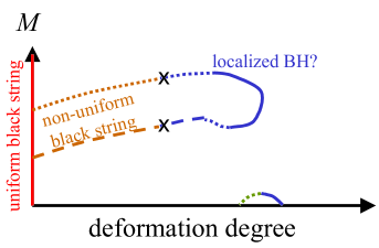
Figure 6: Hypothesized solution sequences for the RS-I model (This figure is taken from Ref. Tanaka:2009zz).

This situation may look a little unnatural. If we assume that there is no static localized black hole solution larger than $\mathcal{O}(\ell)$ also in the RS-I model. Then, to be compatible with this assumption, the reconnection of the sequences as shown in Fig. 6 should take place: the two different sequences of a non-uniform black string will be connected to each other forming a loop, while the sequence of a localized black hole is merged with that of a floating black hole.

Now, the case of the RS-II model is obtained by taking the IR brane to infinity in the RS-I model. Since the wavelength of the lowest Gregory-Laflamme instability mode is infinitely long in this limit, the solution sequences for the non-uniform black strings will disappear from the solution phase diagram. As a result, only the sequence of a brane-localized black hole with/without a maximum size will remain in Fig. 6/Fig. 4. Such a phase structure Fig. 6 is consistent with the classical evaporation conjecture.

5.1.3 Evaporation time scale and astrophysical constraints on $\ell$

Here, we study the evaporation rate of a black hole of mass $M$ due to the Hawking radiation through a single quantum field. Since the Hawking radiation is approximated by black body radiation at the temperature $T=(8\pi G_{4}M)^{-1}$, its radiation flux is given by $F=\pi^{2}T^{4}/60$. Multiplying the black hole horizon area $A=4\pi(2G_{4}M)^{2}$, we obtain the mass loss rate $\dot{M}$ as $\dot{M}=-(15360\pi G_{4}^{2}M^{2})^{-1}\equiv-C/M^{2}$. Solving this relation, we find that the black hole mass varies as $M(t)=(-3Ct)^{1/3}$. Then, the evaporation time $t_{\text{evap}}$ of a black hole with mass $M$ is estimated as $t_{\text{evap}}=M^{3}/{3C}=2.10\times 10^{67}\left({M/M_{\odot}}\right)^{3}\,\mathrm{years},$ where $M_{\odot}$ is the solar mass. It implies that only the black holes lighter than $10^{-19}M_{\odot}\sim 10^{11}\mathrm{kg}$ can evaporate within the Hubble time, $H^{-1}\sim 10^{10}\,\mathrm{years}$. If we take into account the degrees of freedom of the strongly-coupled CFT, which is given by $N^{2}\approx\pi\ell^{2}/G_{4}=2.36\times 10^{60}\times(\ell/14\mu\mathrm{m})^{2}$, the radiation power is multiplied by $15N^{2}\times(3/4)$ and the evaporation time is altered to

$$t_{\text{evap}}^{\text{CFT}}=7.91\times 10^{5}\times\left(\frac{14\,\mu\mathrm{m}}{\ell}\right)^{2}\left(\frac{M}{M_{\odot}}\right)^{3}\mathrm{years}=155\times\left(\frac{1\,\mathrm{mm}}{\ell}\right)^{2}\left(\frac{M}{M_{\odot}}\right)^{3}\mathrm{years}~{}.$$ (57)

We adopted $14\,\mu\text{m}$ as the normalization of $\ell$, which is the current upper bound on $\ell$ obtained from table-top experiments [129, 130, 131].

The evaporation rate of the same order of magnitude can be explained also in the five-dimensional picture assuming the Gregory-Laflamme-type instability at the tip of the horizon [115]. Namely, such instability will create blobs of horizon of the size $\ell^{3}$ within dynamical time scale $G_{4}M$, and then the five-dimensional horizon area $\sim M^{2}\ell$ will decrease as $\frac{d}{dt}M^{2}\ell\approx\ell^{3}/G_{4}M$. This implies $\dot{M}\approx\ell^{2}/G_{4}M$, which coincides with the four-dimensional estimation of $\dot{M}$.

Equation (57) relates the lifetime of a black hole with the bulk curvature scale $\ell$. Thus, if we could give a lower bound on the lifetime of a black hole, we can translate it to the upper bound on $\ell$. Since the typical black hole life time according to Eq. (57) is very short in the cosmological sense, we have a good chance to obtain an extremely stringent upper bound on $\ell$ if it really holds. One problem is that it is difficult in general to measure the life time or its mass loss of a black hole observationally.

Some attempts to give bounds on $\ell$ using this conjecture were made by Refs. 2009ApJ…691..997J and 2009A&A…507..617J. They focused on X-ray binaries, and estimated evaporation rate of the black holes from change in orbital periods of the binaries. In this way, they obtained a bound $\ell\lesssim 0.132\,\text{mm}$. Another approach was given in Refs. 2009ApJ…705L.168G and 2008ApJ…683L.139Z, in which the age of a black hole was estimated from observations of its host globular cluster. They claim that they could give a bound $\ell\lesssim 0.003\,\text{mm}$, though there are many subtle issues in the observations and the logic they used to obtain this bound. Recently, Ref. 2009arXiv0912.4744M suggested a possibility that gravitational wave observations using LISA on the event rate of the extreme mass ratio inspirals or the detection of a single galactic black hole binary may give an upper bound $\ell\lesssim 20\,\mu\text{m}$. Reference Yagi:2011yu focused on correction to the gravitational waveform due to the black hole evaporation and usage of gravitational wave observatory such as DECIGO [138, 139] or BBO [140] which are capable of detecting $10^{5}$ neutron star/black hole binaries per year. It was shown that statistical analysis using them can give an upper bound $\ell\lesssim 0.33\,\mu\text{m}$ after $5$ years of observation.

5.2 Analytic approaches

We summarize analytic approaches to the black hole solutions in the RS-II model and the bulk/brane correspondence about it in this section. We first mention the exact solution in the lower-dimensional model in §5.2.1, and then introduce perturbative approaches and near-horizon analysis in §§5.2.2 and 5.2.3, respectively.

5.2.1 Exact solutions in lower-dimensional model

There is no known analytic solution of a black object in the five-dimensional RS-II model, except for the black string [118]. However, in the lower-dimensional RS-II model with AdS₄ bulk and $(1+2)$-dimensional brane, exact solutions of brane-localized black holes do exist [141].

The exact solutions are constructed from the AdS C-metric, whose metric is given by

$$ds^{2}=\frac{\ell^{2}}{\left(x-y\right)^{2}}\left[-Fdt^{2}+\frac{dy^{2}}{F}+\frac{dx^{2}}{G}+Gd\varphi^{2}\right]~{},$$ (58)

$$F=y^{2}+2\mu y^{3},\;\;\;G=1-x^{2}-2\mu x^{3},$$ (59)

with $\mu\geq 0$. The coordinates in this metric can be assimilated to ordinary polar coordinates $(r,\theta)$ by $y\sim r^{-1}$ and $x\sim\cos\theta$. As shown in Fig. 7, the brane is located at $x=0$. An important property of this solution is that the extrinsic curvature of the $x=0$ hypersurface is the induced metric multiplied by $1/\ell$. Therefore, cutting the solution and gluing it with its copy, we obtain a surface that satisfies the required junction conditions. Thus, one can regard this plane as a $(1+2)$-dimensional brane with constant tension.

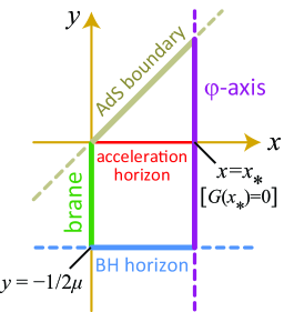
Figure 7: Range of coordinates of the four-dimensional brane-localized black hole.

The range of the coordinate $x$ is bounded by $x_{*}$, the unique positive real root of $G(x)=0$. The boundary at $x=x_{*}$ corresponds to the axis of $\varphi$-rotation. Requiring the regularity on the axis, the period of the angular coordinate $\varphi$ is fixed as

$$\Delta\varphi=\frac{4\pi}{|G^{\prime}(x_{*})|}~{}.$$ (60)

Notice that $\Delta\varphi\leq 2\pi$ and the equality holds for $\mu=0$. The black hole horizon is located at $y=-1/2\mu$. The AdS boundary and the acceleration horizon of the Poincare patch is given by $x=y$ and $y=0$, respectively. If the brane is removed, this solution describes an accelerating black hole solution pulled by a cosmic string in asymptotically AdS spacetime[142, 143].

This exact solution, however, is different from a brane-localized black hole in the five-dimensional RS-II model in many regards:

• The induced geometry on the $(1+2)$-dimensional brane, which is given by

  $$ds^{2}=-\left(1-\frac{2\mu\ell}{r}\right)dt^{2}+\left(1-\frac{2\mu\ell}{r}\right)dr^{2}+r^{2}d\varphi^{2}~{},$$ (61)

  does not resemble a solution in three-dimensional gravity, in which a massive source can create only a locally-flat conical geometry. The appearance of a black hole solution in the present setup is really a four-dimensional phenomenon, and it may be attributed to the quantum effect of CFT in the dual language. The effective energy-momentum tensor derived from the geometry induced on the brane, which is given by

  $$T_{\mu\nu}\simeq-\frac{1}{8\pi G_{3}}E_{\mu\nu}~{},\qquad E_{\mu\nu}=\frac{\mu\ell}{r^{3}}\text{diag}\left(1,1,-2\right)~{},$$ (62)

  is consistent with the one generated by CFT fields with $\mathcal{O}\left(\pi\ell^{2}/G_{3}\right)$ degrees of freedom [115, 116] in the spacetime with a deficit angle.

• The asymptotic geometry at large radii ($y\to 0$) varies depending on the values of $\mu$. If we send $y$ to 0 so as not to hit the acceleration horizon, it should go to the point $y=0=x$. Around this point, the apparent $\mu$-dependent terms in the metric (58) are all irrelevant. However, the difference of $\Delta\varphi$ from $2\pi$ persists. Therefore it is clear that the asymptotic structure significantly changes depending on $\mu$. This feature is not expected in the five-dimensional RS-II model.

• Similarly, one can also compute the Kretschmann invariant of the C-metric to be given by

  $$R_{\mu\nu\rho\lambda}R^{\mu\nu\rho\lambda}=\frac{24}{\ell^{4}}+\frac{48\mu^{2}\left(x-y\right)^{2}}{\ell^{4}}~{}.$$ (63)

  The first term is the contribution of the bulk cosmological constant, and it coincides with the Kretschmann invariant of pure AdS₄ spacetime. The second term is the contribution of the black hole. The latter vanishes on the AdS boundary $x=y$, but does not on the acceleration horizon $y=0$, having dependence on the azimuthal angular coordinate $x$. This property of remaining Kretschmann invariant on the acceleration horizon is not expected in the five-dimensional RS-II model. In the five-dimensional case, one can tell the expected form of the Kretschmann invariant from the Green’s function given in Eq. (20). It it easy to show that the Kretschmann invariant decays in proportion to $z^{-2}$, vanishing everywhere on the acceleration horizon[15]. The presence of deformation beyond the acceleration horizon would mean that the boundary condition of the problem is different for different $\mu$, which implies that the quantum state might be also different from the standard one in the QFT picture. Although this viewpoint has not been widely accepted, we suspect that this will be the reason why the Hawking radiation is absent in this spacetime in the dual picture, if the black hole evapolation conjecture is correct.

Before moving on to the next topic, let us make comments on some related works. Ref. Nozawa:2008wf found linearized equations for conformal scalar, Maxwell and massless Dirac fields on this background become separable. Using this property, they studied quasi-normal modes for those fields, and found that their radial part coincides with that for four-dimensional Schwarzschild black holes while angular part is modulated due to existence of the brane. There were also some attempts to generalize the solution. In the solution construction explained above, the brane tension could be detuned by changing the parameters of the background C-metric. In this way, exact solutions of black holes in the KR model with asymptotically AdS brane were constructed [145]. Another way of generalization is to modify the way of slicing the C-metric with brane. Such an idea was pursued by Anber and Sorbo [146], and they constructed solutions which can be interpreted in the four-dimensional perspective as a time-dependent CFT lump around a conical singularity or two particles sustained by a string.

5.2.2 Perturbative approach

Another analytical approach to the brane-localized black hole is the perturbative approach, which applies for small mass black holes.

• Matched asymptotic expansion:

  First example of perturbative solutions were constructed by Karasik et al. [147, 148]. When the black hole is small enough compared to the bulk curvature scale, the spacetime near the black hole will be well approximated by a five-dimensional Schwarzschild black hole solution. They perturbed this solution taking $\epsilon$, the ratio of Schwarzschild radius and the bulk curvature length, as a small parameter. The effect of brane tension can be taken into account at the first order in $\epsilon$, and the bulk curvature effect arises only at the second order. They succeeded in constructing a perturbative solution in the near-horizon region to the linear order in $\epsilon$, and matched it to the perturbative solution in the asymptotic region far from the source.

• Accelerating black holes in AdS spacetime:

  Another perturbative approach was made by Kodama [149], which focused on solutions describing accelerating black holes in the AdS spacetime.

  In this study, the gravitational field around a semi-infinite string gravitational source was solved perturbatively on the background of AdS spacetime. As a result, solutions which describe black holes accelerating in asymptotically AdS spacetime were successfully obtained.

  Then, as a next step, it was assessed whether brane-localized black hole solutions in the RS-II model can be constructed by cutting those accelerating black hole solutions, in a similar way with the exact solution construction in the lower-dimensional model [141]. The results are:

  • When the bulk dimension is five or higher, the perturbative solutions corresponding to an accelerating the black hole sourced by a constant tension string along the symmetry axis do not admit slicing with a vacuum brane.

  • When the bulk dimension is four, it is possible to slice the accelerating black hole solution with a constant tension brane even when the tension of the string source is non-constant. It indicates that the perturbative solutions of a brane-localized black hole may have degrees of freedom of a one-dimensional free function.

  If the latter is the case even in the non-linear regime, it means that the black hole uniqueness does not hold in the RS model, at least in the four-dimensions. The author gave an explanation to this breakdown of the uniqueness from the holographic point of view: The Einstein equations suffer from higher-derivative correction (see Eq. (53) and below), which is the quantum correction due to the CFT, and then the uniqueness is violated by them.

5.2.3 Near-horizon analysis

It is generally difficult to construct exact solutions of black objects. The problem, however, can be simplified for extremal horizons, focusing on the near-horizon region due to symmetry enhancement. Such a near-horizon analysis of an extremal horizon was established by Ref. nearhorizon, and the uniqueness of the near-horizon geometry was shown. This analysis method was applied to the brane-localized black hole study in Ref. Kaus.

The recipient of the analysis is a brane-localized black hole which is made to be extremal by gauge fields on the brane. Since the surface gravity has to be constant on the event horizon to maintain its regularity, the event horizon in the bulk must be extremal if it is extremal on the brane. Focusing on this five-dimensional extremal horizon, they successfully constructed the near-horizon geometry of an extremal brane-localized black hole of an arbitrary size. They confirmed that the near horizon geometry of the four-dimensional solution on the brane approaches the ordinary Reissner-Nordstrom (RN) black hole in the large black hole limit and evaluated explicitly the leading deviation from the RN black hole. This analysis is interesting since, though the solution is given only in the near-horizon region, this is the only analytic construction of a brane-localized black hole solution other than that in the lower-dimensional model [141, 145] we mentioned in §5.2.1. The extension of this near-horizon analysis to the KR model case was argued by Ref. Suzuki.

Note that this near-horizon analysis does not guarantee that a static solution in the entire bulk does exist. It will be interesting to confirm the existence of such a static solution, though we probably have to resort to numerical technique similar to Refs. Wiseman:2001xt,Kudoh:2003xz,Kudoh:2004kf,Yoshino:2008rx to construct it.

5.3 Numerical approaches

In this section, we summarize numerical approaches to the issues of brane-localized black holes in the RS-II model. After mentioning some approximative approaches in §5.3.1, we explain the current status of numerical solution construction in §5.3.2.

5.3.1 Approximative approach

Since direct approaches toward numerical solution construction is rather difficult, some approximative approaches for solution construction have been developed. One of such approximative approach was discussed in Ref. Creek:2006je. Their trick is to use a known exact black hole solution for the bulk spacetime metric, and consider the brane trajectory on such a background. One of the background bulk spacetime they used is the five-dimensional AdS Schwarzschild spacetime. Since this bulk does not admit vacuum brane slicing, they put some matter on the brane to force the brane to be static. In this way, they constructed a static solution of a brane-localized black hole in the RS-II model with some artificial matter on the brane.

Another approach is to relax the static condition. By requiring the system to be only momentarily static, instead of being completely static, we can find a vacuum brane slicing on the AdS-Schwarzschild bulk only by solving a set of ordinary differential equations. Such a solution might inherit some properties of static solutions. Static solutions should be contained in the whole set of momentarily-static solutions, and we may expect that a solution with maximum entropy in a whole set of momentarily-static solutions to is a static solution. Based on this idea, Ref. Tanahashi studied the properties of momentarily-static solutions of brane-localized black holes. Although the investigated momentarily-static solutions were very limited, the results were consistent with the classical black hole conjecture of the brane-localized black holes. An extension of this approach to the KR model was discussed in Ref. fBH.

5.3.2 Direct approach to the solution construction

First attempt of numerical solution construction was made by Kudoh et al. [153, 154] based on the numerical technique explained in §4. Solving a set of three elliptic equations numerically by the relaxation method, solutions for small static brane-localized black holes were successfully constructed. However, their numerical code failed to find solutions with the horizon size larger than $\sim 0.2\ell$. Kudoh [154] applied this numerical technique to the brane-localized black holes in six-dimensional RS-II model, and constructed solutions whose size is as large as $\sim 2\ell$.

This numerical analysis was re-analyzed by Yoshino [155]. The improvements are in the choice of coordinates and variables as well as in the accuracy of numerical differentiation. In Ref. Kudoh:2003xz, they used the coordinates $(\rho,\xi)$ defined from Eq. (55) by

$$r=\rho\sin\chi~{},\qquad z=\ell+\rho\cos\chi~{},\qquad\xi=\chi^{2}~{}.$$ (64)

The angular coordinate $\xi$ was employed to eliminate terms proportional to $1/\sin^{2}\chi$, which becomes singular on the axis of rotational symmetry, from the equations. Reference Yoshino:2008rx used coordinates $(x,\chi)$ defined by $x\equiv\log(\rho/\rho_{\text{horizon}})$ instead. $\chi$ was chosen to increase the number of data points near the axis, and $x$ was introduced to let the asymptotic boundary, at which the metric is set to coincide with the unperturbed RS model, much further compared to Ref. Kudoh:2003xz. One drawback of this choice is the re-appearance of singular term $\propto 1/\sin^{2}\chi$. In Ref. Yoshino:2008rx these singular terms were eliminated as far as possible by choosing appropriate linear combinations of the free functions $R$ and $C$ as variables to solve. About the accuracy of differentiation, Ref. Kudoh:2003xz used a scheme with second-order accuracy while Ref. Yoshino:2008rx used one with fourth-order accuracy in the bulk and third-order on the boundaries.

As a result of this numerical analysis, in Ref. Yoshino:2008rx Yoshino claimed that he observed “nonsystematic error”, which is the error distinct from systematic numerical errors due to, e.g., finite grid size or finite distance between the asymptotic boundary and the black hole, and it dominates when the asymptotic boundary is moved toward infinity. Based on this observation, it was guessed that even small static brane-localized black holes may not exist. Ref. Kleihaus:2011yq studied brane-localized black holes charged with respect to a Maxwell field on the brane, and achieved similar results for non-extremal black holes. However, we think that the results in Ref. Yoshino:2008rx are not inconsistent with the existence of small static black holes. When the grid size is reduced, the error reported in Ref. Yoshino:2008rx looks always diminishing for any fixed location of the asymptotic boundary.

Note added: After finishing this review, a paper by Figueras, Lucietti and Wiseman appeared [160]. The paper uses numerical technique based on a version of Ricci-flow equation to solve the static Einstein equations [161], and reports that there is a static black hole solution attached to the AdS boundary with the induced metric is conformal to four-dimensional Schwarzschild black hole. This means that CFT coupled with four-dimensional gravity does not radiate even if there is a black hole at the leading order of $1/N$ expansion. Numerical results of their subsequent paper implies that this solution is smoothly related to brane-localized black hole solutions in the RS-II model [162].

Here we explain our tentative understanding of this result. The result shows that the energy density of CFT increases near the horizon to the level comparable to the radiation fluid composed of $O(N^{2})$ degrees of freedom at the Hawking temperature. In this sense one may say that the pressure of CFT cloud is in balance with the pressure of the Hawking radiation from the black hole horizon. This increase of energy density near the horizon could be expected to some extent by extrapolating the energy density around a point particle, which behaves like $\propto N^{2}r_{g}/r^{5}$, where $r_{g}$ is the gravitational radius of the point particle. Near the horizon, it blows up to $N^{2}/r_{g}^{4}\approx N^{2}T_{BH}^{4}$. The behavior of the CFT cloud around a point particle, which is similar to that for their black hole solution in asymptotic region, however, is far different from radiation fluid. The pressure is comparable to the energy density, decaying proportional to $1/r^{5}$, but it is not isotropic at all. Tangential pressure is negative and $3/2$ times bigger in magnitude than the radial one. The force balance in the radial direction is established essentially between the radial pressure gradient and the tension in the tangential directions. We should note that all of these features can be understood also in terms of the language of weakly coupled CFT. Such CFT contribution to be attributed to the vacuum polarization caused by spacetime curvature would be distinguished from thermal component as in the case of dark radiation. In the latter case one can freely change the amplitude of CFT energy density, and it seems to behave like radiation fluid.

Many new questions arise to obtain a consistent picture to understand the behavior of strongly coupled CFT. The evidences previously supporting the black hole evaporation conjecture as mentioned in this section might be now in conflict with the existence of static black hole solutions. The arguments were mostly based on the analogy of the weakly coupled CFT or radiation fluid. We need to clarify which part of the analogy breaks down.

6 Black holes in other braneworld models

6.1 Black holes in KR model

In the KR model, the geometry on the brane is AdS₄. Let us firstly remind basic properties of black holes in equilibrium with radiation in asymptotically AdS spacetime. The negative cosmological constant of the AdS spacetime exerts contracting force to fields in it. In other words, the effective gravitational potential rises up to infinity at the AdS boundary, and it effectively plays as a bounding box. Then, a quantum black hole in the asymptotic AdS spacetime can be in thermal equilibrium with its Hawking radiation since the emitted radiation is trapped by this gravitational potential well. Furthermore, it is known that black holes larger than the curvature scale of AdS spacetime have positive specific heat and thus they are thermodynamically stable. In contrast, black holes smaller than AdS curvature scale evaporate completely without reaching thermal equilibrium. This implies that there is a phase transition between thermal AdS phase at low temperature and the AdS black hole phase at high temperature. Such phase transition in the canonical or micro-canonical ensemble is known as the Hawking-Page transition [163].

Keeping in mind the above-mentioned properties of black holes in asymptotically AdS spacetime, let us consider the implication of the bulk/brane correspondence on brane-localized black holes in the KR model. (What we consider here seems to be different blanch of solutions that can exist also in RS-II setup. In that case the energy density of CFT vanishes at infinity and is far from the thermal one.) First of all, the bulk/brane correspondence implies that there should be a large static brane-localized black hole as its five-dimensional counterpart. It also predicts that there should be some transition in the bulk spacetime which is dual to the Hawking-Page transition. Such a possibility was firstly considered in Ref. CK, which claimed that the bulk counterpart of the Hawking-Page transition is given by the transition between thermal AdS₅ phase and the five-dimensional AdS black string phase. Since the projection of the AdS black string solution onto the brane is four-dimensional AdS Schwarzschild spacetime, this five-dimensional phase transition is quite in parallel to that in four dimensions.

A five-dimensional black string in AdS spacetime, however, requires infinite energy to be produced from the thermal bath since the black string extends to the AdS boundary and the horizon area and the mass diverge there. Such an infinite energy input is possible in a canonical ensemble with a fixed temperature, but impossible in a micro-canonical ensemble with a fixed total energy. In the actual dynamical gravitational collapse, the amount of energy that can be used is limited. Hence, formation of infinitely long black string is prohibited.

Another scenario of the transition in five dimensions was proposed in Ref. Tanaka:2009zz taking the following points into account.

• The holography implies the existence of a static brane-localized black hole larger than the four-dimensional bulk curvature scale on the brane.

• Since the KR model can be obtained by smooth deformation of the RS model, i.e., by decreasing the brane tension, the phase diagram of black objects in the KR model must be smoothly connected to that in the RS model.

• Since black string solutions cannot be obtained with a finite amount of energy, they are not included in the phase diagram of solutions as long as equilibrium states in the micro-canonical ensemble are concerned.

To consider the bulk black holes in the KR model, let us first examine properties of a particle placed in the bulk of this model. It is convenient to introduce the coordinates given by

$$ds^{2}=dy^{2}+\ell^{2}\cosh^{2}\left(y/\ell\right)ds^{2}_{\text{AdS}_{4}}~{},$$ (65)

where $ds^{2}_{\text{AdS}_{4}}$ is the metric of AdS₄ with unit curvature. The particle placed in the bulk will feel acceleration due to the bulk cosmological constant, and its value will be given by $a=\left(\log\sqrt{-g_{tt}}\right)_{,y}$. Then, the effective gravitational potential due to the warped bulk geometry will be given by

$$U_{\text{eff}}=\log\left(\sqrt{-g_{tt}}\right)=\log\left\{\ell\cosh\left(\frac{y}{\ell}\right)\right\}~{}.$$ (66)

In addition to that, the gravitational attraction between the particle and its mirror image will also contribute to the effective potential. The total effective potential for a small particle in the bulk will be schematically as shown in Fig. 8. This effective potential will have two extrema at which the small particle can stay at rest: a stable minimum at the “throat” of the bulk and an unstable maximum near the brane.

Figure 8: Effective potential for a small particle in the KR model bulk. (This figure is taken from Ref. Tanaka:2009zz.)

Now we will consider black hole solutions in the bulk. When the black hole is sufficiently small, it will be approximated simply by a point particle. Then, the effective gravitational potential for this small black hole will be similar to that for a point particle shown in Fig. 8. Corresponding to the two extrema in the effective potential, there will be two solutions for such a small black hole for a fixed mass, and thus there will be two sequences of solutions of a floating small black hole. One sequence represents a black hole staying at the unstable maximum near the brane, and the other represents the one staying at the stable minimum at the “throat” of the bulk.

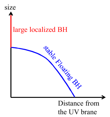
Figure 9: Proposed phase diagram of the black hole solution sequences in the KR model.

To get a perspective on the entire solution sequences, let us consider what will happen when we increase the black hole mass. First, we study a black hole at the unstable maximum. Since that black hole is sustained by gravitational attraction from its mirror image behind the brane, its properties will be similar to those of a floating black hole in the RS-II model (see §5.1.2). Next, we study a black hole at the stable minimum, which is located at the “throat” of the bulk. Such a black hole will sit there until it becomes sufficiently large to fill up the region between the “throat” and the brane. Increasing further the black hole mass, the black hole will touch the brane and then it will become a brane-localized black hole. We summarize the latter solution sequence deduced from the above consideration in Fig. 9.

Let us consider further how the solutions in the latter sequence look like on the brane and the stability of those solutions in the five-dimensional point of view. When the black hole larger than the bulk curvature scale is floating near the “throat” in the bulk, the temperature of the black hole increases as we increase the mass of the black hole. (Notice that the surface gravity of an AdS black hole increases as its mass becomes bigger when the size is bigger than the AdS curvature length.) In the four-dimensional dual picture, the energy-momentum tensor due to QFT will be approximated by that of radiation fluid with a large number of degrees of freedom in thermal equilibrium at the black hole temperature, and hence the energy density will increase as the black hole becomes bigger. At some critical size, the bulk black hole will touch the brane. The intersection of the five-dimensional black hole with the brane will be observed from a brane observer as a four-dimensional black hole associated with surrounding radiation. Such a configuration with a large five-dimensional black hole and a small four-dimensional intersection looks unstable. By increasing the five-dimensional black hole size further, the size of the four-dimensional black hole will become larger than the four-dimensional AdS curvature scale. In this regime, the solution will look like the black string solution truncated at around the “throat”. Such a five-dimensional black hole with a large four-dimensional intersection will be stable.

Assuming the bulk/boundary correspondence, we can estimate the physical parameters at the critical points. Firstly, the size of the five-dimensional black hole when it touches the brane is estimated as follows. When the five-dimensional black hole touches the brane, the temperature at the touching point will diverge since local temperature is proportional to the red-shift factor $1/\sqrt{-g_{tt}}$. In the four-dimensional dual picture, this configuration would be described by self-gravitating radiation fluid whose density diverges at the center. Properties of such radiation fluid star in asymptotically AdS spacetime was studied by Ref. PP, and it was shown that such a star with singular central density has entropy of $\mathcal{O}\left(G_{4}^{-1}\ell^{1/2}L^{3/2}\right)$. This entropy should coincide with the five-dimensional entropy $S\sim A_{5}/G_{5}\sim A_{5}/\left(\ell G_{4}\right)$ if the bulk/brane correspondence holds. Assuming so, we find that the five-dimensional black hole area and the five-dimensional black hole radius at this critical point to be $A_{5}\sim\left(\ell L\right)^{3/2}$ and $r_{\text{5DBH}}\sim(\ell L)^{1/2}$, respectively.

Next, we estimate the size of a large brane-localized black hole at the transition of stability. Again, in the dual four-dimensional picture, a black hole is stable when its mass becomes comparable to the total radiation energy around the black hole, $N^{2}T^{4}L^{3}\sim G_{4}^{-1}\ell^{2}L^{3}T^{4}$. Then, the critical temperature will be given by $T\sim(\ell^{2}L^{3})^{-1/5}$, where we used $M\sim(G_{4}T)^{-1}$ assuming $T\ll L^{-1}$. Then, the critical mass and horizon radius will be given by $M\sim G_{4}^{-1}(\ell^{2}L^{3})^{1/5}$ and $r_{\text{4DBH}}\sim(\ell^{2}L^{3})^{1/5}$, respectively. This $r_{\text{4DBH}}$ will be the critical radius of the intersection of the brane and the brane-localized black hole. In Ref. Kashiyama, the above estimates were conducted more explicitly in the four-dimensional point of view using radiation fluid approximation, taking into account the back reaction to the geometry.

These expectations about the solution sequences was studied in Ref. fBH from the five-dimensional point of view. In this work, time-symmetric initial data of five-dimensional black hole floating in the bulk of the KR model was constructed, and its properties, such as thermodynamic stability or effective energy density profile induced on the brane, were studied. The results basically supported the arguments presented above based on the bulk/brane correspondence.

Note Added: Here we assumed that the black holes are in thermal equilibrium with the CFT cloud. This expectation might be wrong from the fact that there are brane-localized black hole solutions in RS-II model, which are not in equilibrium in the sense that the asymptotic energy density of CFT vanishes. However, even in that case one can argue that local pressure balance between the black hole radiation and the surrounding cloud is satisfied. Furthermore, the existence of the sequence of solutions discussed in this subsection is naturally expected from the consideration in five-dimensional gravity side without relying on the bulk/brane correspondence.

6.2 Black holes in DGP model

The perturbative analysis of gravity in the DGP model requires a special care since a naive perturbative expansion around a pure four-dimensional solution breaks down in the short scale $r\ll r_{*}$. Thanks to some studies, it was noticed that it is the brane bending which becomes non-linear in this range, and that the perturbative analysis can be accomplished only by taking the second order perturbation with respect to the brane bending at least when matter source is sufficiently smoothed out. This analysis indicates that the gravitational field around a source of four-dimensional mass $M$ is roughly given as summarized in Table 1.

Table 1: Gravitational field of mass $M$ in the DGP model clarified by a perturbative analysis.

$r_{g}\ll r\ll r_{*}$	four-dimensional Schwarzschild solution for mass $M$
$r_{*}\ll r\ll r_{c}$	solution interpolating four and five-dimensional solutions
$r_{c}\ll r$	five-dimensional Schwarzschild solution for mass $M$

A perturbative analysis, however, does not apply to general matter source and breaks down especially in region $r\sim r_{g}$ where the solution will become non-linear. To investigate the gravity in this region, we have to solve the Einstein equations non-perturbatively to construct a black hole solution. This direct approach is not accomplished so far.

An approximative method that simplifies the problem is to introduce an ad-hoc metric ansatz. Such an attempt was done in Ref. Middleton:2003yr and approximate solutions including the region $r\sim r_{g}$ were obtained. Using another ansatz $-g_{tt}=1/g_{rr}$ on the brane, the authors of Ref. G-Sch extracted a closed equation of the lapse function on the brane from the full Einstein equations. By solving this equation, they fixed the induced metric and a part of extrinsic curvature on the brane. The difference of their result from the perturbative result summarized in Table 1 is in the long range region $r\gg r_{*}$. Their solution converges into a five-dimensional Schwarzschild spacetime not with $M$ but with a screened mass $M\left(r_{g}/r_{c}\right)^{1/3}$.

An alternative approach to study the gravitational field in the DGP model is to use the shockwave solutions, which describes a gravitational field induced by a particle on the brane moving in a relativistic speed. One advantage of this approach is that exact solutions in the entire bulk can be obtained by rather simple analysis. This analysis showed that the interpolation between four-dimensional behavior in short scale and five-dimensional one in large scale does persist even in the presence of dynamical gravity generated by Planckian scattering of particles [170, 171]. This approach may provide a new window to non-linear gravitation in the DGP model.

7 Summary and outlook

In this review, we introduced basics about representative braneworld models and their gravitational properties, and summarized current understandings about black hole solutions in those models. Perturbative gravity is well understood in these braneworld models, but black hole solutions are less known yet. In particular, explicit numerical construction of solutions in the models with a warped extra-dimension such as the RS model and the KR model is still very limited. We therefore invoked arguments based on the bulk/brane correspondence in braneworld models, to predict the features of black hole solutions in such models.

The primary interest in this context would be to prove the bulk/brane correspondence in braneworld models, which seems difficult to accomplish in a formal way, though. The bulk/brane correspondence in braneworld naively predicts classical evaporation of a brane-localized black hole in the RS-II braneworld model. This prediction, however, very recently seems to be denied by a beautiful numerical study by P. Figueras, J. Lucietti and T. Wiseman, although further confirmation by independent calculation is wanted. The solution they have provided indicates that CFT can be in equilibrium with a black hole without emitting Hawking radiation at the leading order of the so-called large $N$ expansion. This proves that this field of research is still very active, and that this review is really written in the middle stage of rapid growth. We hope that this review provides a guide for further development.

Studies of black holes in the modified setup, such as braneworld models with bulk Gauss-Bonnet term or the DGP braneworld model, would be also very fruitful, though such studies are rather limited at this moment compared to those for the RS model. It would be interesting to study the properties of black hole solutions or the holography in these modified settings, too.

References

- [1] T. Kaluza, Sitzungsber. Preuss. Akad. Wiss. Berlin (Math. Phys.) (1921), 966.
- [2] O. Klein, Z. Phys. 37 (1926), 895.
- [3] N. Arkani-Hamed, S. Dimopoulos and G. R. Dvali, Phys. Lett. B 429 (1998), 263.
- [4] N. Arkani-Hamed, S. Dimopoulos and G. R. Dvali, Phys. Rev. D 59 (1999), 086004.
- [5] L. Randall and R. Sundrum, Phys. Rev. Lett. 83 (1999), 3370.
- [6] L. Randall and R. Sundrum, Phys. Rev. Lett. 83 (1999), 4690.
- [7] G. R. Dvali, G. Gabadadze and M. Porrati, Phys. Lett. B 485 (2000), 208.
- [8] J. M. Maldacena, Adv. Theor. Math Phys. 2 (1998), 231.
- [9] O. Aharony, S. S. Gubser, J. M. Maldacena, H. Ooguri and Y. Oz, Phys. Rep. 323 (2000), 183.
-
[10]
E. Witten, Remarks at ITP Santa Barbara conference, “New Dimensions
in Field Theory and String Theory,” (1999).
http://www.itp.ucsb.edu/online/susy_c99/discussion/ -
[11]
H. L. Verlinde, Invited talk at ITP Santa Barbara conference, “New
Dimensions in Field Theory and String Theory,” (1999).
http://www.itp.ucsb.edu/online/susy_c99/discussion/ - [12] G. D. Kribs, hep-ph/0605325.
- [13] H. C. Cheng, arXiv:1003.1162.
- [14] I. Antoniadis, N. Arkani-Hamed, S. Dimopoulos and G. R. Dvali, Phys. Lett. B 436 (1998), 257.
- [15] J. Garriga and T. Tanaka, Phys. Rev. Lett. 84 (2000), 2778.
- [16] A. Karch and L. Randall, J. High Energy Phys. 05 (2001), 008.
- [17] A. Karch and L. Randall, Phys. Rev. Lett. 87 (2001), 061601.
- [18] A. Karch and L. Randall, J. High Energy Phys. 06 (2001), 063.
- [19] O. DeWolfe, D. Z. Freedman and H. Ooguri, Phys. Rev. D 66 (2002), 025009.
- [20] O. Aharony, O. DeWolfe, D. Z. Freedman and A. Karch, J. High Energy Phys. 07 (2003), 030.
- [21] N. Kaloper and L. Sorbo, J. High Energy Phys. 08 (2005), 070.
- [22] U. Gen and M. Sasaki, Prog. Theor. Phys. 105 (2001), 591.
- [23] N. Kaloper, Phys. Rev. D 60 (1999), 123506.
- [24] T. Nihei, Phys. Lett. B 465 (1999), 81.
- [25] Y. Iwashita, T. Kobayashi, T. Shiromizu and H. Yoshino, Phys. Rev. D 74 (2006), 064027.
- [26] N. D. Birrell and P. C. W. Davies, Quantum Fields in Curved Space (Cambridge University Press, Cambridge, 1982).
- [27] C. Deffayet, Phys. Lett. B 502 (2001), 199.
- [28] C. Deffayet, G. R. Dvali and G. Gabadadze, Phys. Rev. D 65 (2002), 044023.
- [29] V. Sahni and Y. Shtanov, J. Cosmol. Astropart. Phys. 11 (2003), 014.
- [30] A. Nicolis, R. Rattazzi and E. Trincherini, Phys. Rev. D 79 (2009), 064036.
- [31] K. Koyama, Phys. Rev. D 72 (2005), 123511.
- [32] C. Charmousis, R. Gregory, N. Kaloper and A. Padilla, J. High Energy Phys. 10 (2006), 066.
- [33] D. Gorbunov, K. Koyama and S. Sibiryakov, Phys. Rev. D 73 (2006), 044016.
- [34] K. Izumi, K. Koyama and T. Tanaka, J. High Energy Phys. 04 (2007), 053.
- [35] R. Gregory, N. Kaloper, R. C. Myers and A. Padilla, J. High Energy Phys. 10 (2007), 069.
- [36] R. Gregory, Prog. Theor. Phys. Suppl. No. 172 (2008), 71.
- [37] K. Izumi and T. Tanaka, Prog. Theor. Phys. 121 (2009), 419.
- [38] K. Izumi and T. Tanaka, Prog. Theor. Phys. 121 (2009), 427.
- [39] C. Deffayet, G. R. Dvali, G. Gabadadze and A. I. Vainshtein, Phys. Rev. D 65 (2002), 044026.
- [40] M. A. Luty, M. Porrati and R. Rattazzi, J. High Energy Phys. 09 (2003), 029.
- [41] G. Dvali, New J. Phys. 8 (2006), 326.
- [42] T. Tanaka, Mod. Phys. Lett. A 25 (2010), 936.
- [43] Y. Iwasaki, Phys. Rev. D 2 (1970), 2255.
- [44] H.v. Dam and M. J. G. Veltman, Nucl. Phys. B 22 (1970), 397.
- [45] V. I. Zakharov, JETP Lett. 12 (1970), 312.
- [46] A. I. Vainshtein, Phys. Lett. B 39 (1972), 393.
- [47] A. Gruzinov, New Astron. 10 (2005), 311.
- [48] T. Tanaka, Phys. Rev. D 69 (2004), 024001.
- [49] T. Shiromizu, K. i. Maeda and M. Sasaki, Phys. Rev. D 62 (2000), 024012.
- [50] W. Israel, Nuovo Cim. B 44 (1966), 1.
- [51] T. Shiromizu, T. Torii and D. Ida, J. High Energy Phys. 03 (2002), 007.
- [52] S. Kanno and J. Soda, Phys. Rev. D 66 (2002), 043526.
- [53] P. L. McFadden and N. Turok, Phys. Rev. D 71 (2005), 021901.
- [54] J. Soda, arXiv:1001.1011.
- [55] K. i. Maeda, S. Mizuno and T. Torii, Phys. Rev. D 68 (2003), 024033.
- [56] J. M. Maldacena, hep-th/0309246.
- [57] E. D’Hoker and D. Z. Freedman, hep-th/0201253.
- [58] C. V. Johnson, D-Branes (Cambridge University Press, Cambridge, 2002).
- [59] K. Becker, M. Becker and J. H. Schwarz, String Theory and M-Theory: A Modern Introduction (Cambridge University Press, Cambridge, 2007).
- [60] S. S. Gubser, Phys. Rev. D 63 (2001), 084017.
- [61] S. W. Hawking, T. Hertog and H. S. Reall, Phys. Rev. D 62 (2000), 043501.
- [62] I. Savonije and E. P. Verlinde, Phys. Lett. B 507 (2001), 305.
- [63] G. W. Gibbons and S. W. Hawking, Phys. Rev. D 15 (1977), 2738.
- [64] J. Garriga and M. Sasaki, Phys. Rev. D 62 (2000), 043523.
- [65] M. J. Duff and J. T. Liu, Class. Quant. Grav. 18 (2001), 3207.
- [66] P. R. Anderson, R. Balbinot and A. Fabbri, Phys. Rev. Lett. 94 (2005), 061301.
- [67] P. R. Anderson and A. Fabbri, Phys. Rev. D 75 (2007), 044015.
- [68] T. Tanaka, gr-qc/0402068.
- [69] L. Grisa and O. Pujolas, J. High Energy Phys. 06 (2008), 059.
- [70] S. R. Das and A. Zelnikov, Phys. Rev. D 64 (2001), 104001.
- [71] A. Hebecker and J. March-Russell, Nucl. Phys. B 608 (2001), 375.
- [72] N. Arkani-Hamed, M. Porrati and L. Randall, J. High Energy Phys. 08 (2001), 017.
- [73] M. Porrati, J. High Energy Phys. 04 (2002), 058.
- [74] M. Porrati, Mod. Phys. Lett. A 18 (2003), 1793.
- [75] M. Porrati, Phys. Rev. D 65 (2002), 044015.
- [76] M. J. Duff, J. T. Liu and H. Sati, Phys. Rev. D 69 (2004), 085012.
- [77] R. Bousso and L. Randall, J. High Energy Phys. 04 (2002), 057.
- [78] B. Kol, Phys. Rep. 422 (2006), 119.
- [79] T. Harmark and N. A. Obers, hep-th/0503020.
- [80] S. Dimopoulos and G. L. Landsberg, Phys. Rev. Lett. 87 (2001), 161602.
- [81] P. Kanti, Int. J. Mod. Phys. A 19 (2004), 4899.
- [82] R. Emparan, G. T. Horowitz and R. C. Myers, Phys. Rev. Lett. 85 (2000), 499.
- [83] V. P. Frolov and D. Stojkovic, Phys. Rev. Lett 89 (2002), 151302.
- [84] V. P. Frolov and D. Stojkovic, Phys. Rev. D 67 (2003), 084004.
- [85] A. Flachi and T. Tanaka, Phys. Rev. Lett. 95 (2005), 161302.
- [86] A. Flachi, O. Pujolas, M. Sasaki and T. Tanaka, Phys. Rev. D 73 (2006), 125017.
- [87] A. Flachi, O. Pujolas, M. Sasaki and T. Tanaka, Phys. Rev. D 74 (2006), 045013.
- [88] A. R. Bogojevic and L. Perivolaropoulos, Mod. Phys. Lett. A 6 (1991), 369.
- [89] D. Korotkin and H. Nicolai, gr-qc/9403029.
- [90] A. V. Frolov and V. P. Frolov, Phys. Rev. D 67 (2003), 124025.
- [91] B. Kol, E. Sorkin and T. Piran, Phys. Rev. D 69 (2004), 064031.
- [92] E. Sorkin, B. Kol and T. Piran, Phys. Rev. D 69 (2004), 064032.
- [93] H. Kudoh and T. Wiseman, Prog. Theor. Phys. 111 (2004), 475.
- [94] H. Kudoh and T. Wiseman, Phys. Rev. Lett. 94 (2005), 161102.
- [95] D. Gorbonos and B. Kol, J. High Energy Phys. 06 (2004), 053.
- [96] D. Karasik, C. Sahabandu, P. Suranyi and L. C. R. Wijewardhana, Phys. Rev. D 71 (2005), 024024.
- [97] T. Harmark, Phys. Rev. D 69 (2004), 104015.
- [98] T. Harmark and N. A. Obers, J. High Energy Phys. 05 (2002), 032.
- [99] R. Gregory and R. Laflamme, Phys. Rev. Lett. 70 (1993), 2837.
- [100] R. Gregory and R. Laflamme, Nucl. Phys. B 428 (1994), 399.
- [101] S. S. Gubser, Class. Quant. Grav. 19 (2002), 4825.
- [102] E. Sorkin, Phys. Rev. Lett. 93 (2004), 031601.
- [103] T. Wiseman, Class. Quant. Grav. 20 (2003), 1137.
- [104] B. Kleihaus, J. Kunz and E. Radu, J. High Energy Phys. 06 (2006), 016.
- [105] E. Sorkin, Phys. Rev. D 74 (2006), 104027.
- [106] T. Wiseman, Phys. Rev. D 65 (2002), 124007.
- [107] B. Kol, J. High Energy Phys. 10 (2005), 049.
- [108] T. Tanaka, Prog. Theor. Phys. 121 (2009), 1133.
- [109] G. T. Horowitz and K. Maeda, Phys. Rev. Lett. 87 (2001), 131301.
- [110] D. Marolf, Phys. Rev. D 71 (2005), 127504.
- [111] M. W. Choptuik, L. Lehner, I. Olabarrieta, R. J. W. Petryk, F. Pretorius and H. Villegas, Phys. Rev. D 68 (2003), 044001.
- [112] D. Garfinkle, L. Lehner and F. Pretorius, Phys. Rev. D 71 (2005), 064009.
- [113] L. Lehner and F. Pretorius, Phys. Rev. Lett. 105 (2010), 101102.
- [114] N. Kaloper and D. Kiley, J. High Energy Phys. 03 (2006), 077.
- [115] T. Tanaka, Prog. Theor. Phys. Suppl. No. 148 (2003), 307.
- [116] R. Emparan, A. Fabbri and N. Kaloper, J. High Energy Phys. 08 (2002), 043.
- [117] S. W. Hawking, Commun. Math. Phys. 43 (1975), 199.
- [118] A. Chamblin, S. W. Hawking and H. S. Reall, Phys. Rev. D 61 (2000), 065007.
- [119] R. Gregory, Class. Quant. Grav. 17 (2000), L125.
- [120] R. Gregory, V. A. Rubakov and S. M. Sibiryakov, Class. Quant. Grav. 17 (2000), 4437.
- [121] A. L. Fitzpatrick, L. Randall and T. Wiseman, J. High Energy Phys. 11 (2006), 033.
- [122] S. A. Hartnoll, C. P. Herzog and G. T. Horowitz, J. High Energy Phys. 12 (2008), 015.
- [123] D. T. Son and A. O. Starinets, J. High Energy Phys. 03 (2006), 052.
- [124] A. Chamblin, H. S. Reall, H. a. Shinkai and T. Shiromizu, Phys. Rev. D 63 (2001), 064015.
- [125] R. Emparan, J. Garcia-Bellido and N. Kaloper, J. High Energy Phys. 01 (2003), 079.
- [126] S. S. Gubser, I. R. Klebanov and A. W. Peet, Phys. Rev. D 54 (1996), 3915.
- [127] O. Pujolas, J. High Energy Phys. 12 (2008), 057.
- [128] K. Murata, T. Nishioka, N. Tanahashi and H. Yumisaki, Prog. Theor. Phys. 120 (2008), 473.
- [129] D. J. Kapner, T. S. Cook, E. G. Adelberger, J. H. Gundlach, B. R. Heckel, C. D. Hoyle and H. E. Swanson, Phys. Rev. Lett. 98 (2007), 021101.
- [130] E. G. Adelberger, B. R. Heckel, S. Hoedl, C. D. Hoyle, D. J. Kapner and A. Upadhye, Phys. Rev. Lett. 98 (2007), 131104.
- [131] E. G. Adelberger, J. H. Gundlach, B. R. Heckel, S. Hoedl and S. Schlamminger, Prog. Part. Nucl. Phys. 62 (2009), 102.
- [132] T. Johannsen, D. Psaltis and J. E. McClintock, Astrophys. J. 691 (2009), 997.
- [133] T. Johannsen, Astron. Astrophys. 507 (2009), 617.
- [134] O. Y. Gnedin, T. J. Maccarone, D. Psaltis and S. E. Zepf, Astrophys. J. 705 (2009), L168.
- [135] S. E. Zepf, D. Stern, T. J. Maccarone, A. Kundu, M. Kamionkowski, K. L. Rhode, J. J. Salzer, R. Ciardullo and C. Gronwall, Astrophys. J. 683 (2008), L139.
- [136] S. T. McWilliams, Phys. Rev. Lett. 104 (2010), 141601.
- [137] K. Yagi, N. Tanahashi and T. Tanaka, Phys. Rev. D 83 (2011), 084036.
- [138] N. Seto, S. Kawamura and T. Nakamura, Phys. Rev. Lett. 87 (2001), 221103.
- [139] S. Kawamura, T. Nakamura, M. Ando, N. Seto, K. Tsubono et al., Class. Quant. Grav. 23 (2006), S125.
- [140] E. S. Phinney et al., “Big Bang Observer,” Mission Concept Study (NASA, 2003).
- [141] R. Emparan, G. T. Horowitz and R. C. Myers, J. High Energy Phys. 01 (2000), 007.
- [142] O. J. C. Dias and J. P. S. Lemos, Phys. Rev. D 67 (2003), 064001.
- [143] P. Krtous, Phys. Rev. D 72 (2005), 124019.
- [144] M. Nozawa and T. Kobayashi, Phys. Rev. D 78 (2008), 064006.
- [145] R. Emparan, G. T. Horowitz and R. C. Myers, J. High Energy Phys. 01 (2000), 021.
- [146] M. Anber and L. Sorbo, J. High Energy Phys. 07 (2008), 098.
- [147] D. Karasik, C. Sahabandu, P. Suranyi and L. C. R. Wijewardhana, Phys. Rev. D 69 (2004), 064022.
- [148] D. Karasik, C. Sahabandu, P. Suranyi and L. C. R. Wijewardhana, Phys. Rev. D 70 (2004), 064007.
- [149] H. Kodama, Prog. Theor. Phys. 120 (2008), 371.
- [150] H. K. Kunduri, J. Lucietti and H. S. Reall, Class. Quant. Grav. 24 (2007), 4169.
- [151] A. Kaus and H. S. Reall, J. High Energy Phys. 05 (2009), 032.
- [152] R. Suzuki, T. Shiromizu and N. Tanahashi, Phys. Rev. D 82 (2010), 085029.
- [153] H. Kudoh, T. Tanaka and T. Nakamura, Phys. Rev. D 68 (2003), 024035.
- [154] H. Kudoh, Phys. Rev. D 69 (2004), 104019.
- [155] H. Yoshino, J. High Energy Phys. 01 (2009), 068.
- [156] S. Creek, R. Gregory, P. Kanti and B. Mistry, Class. Quant. Grav. 23 (2006), 6633.
- [157] N. Tanahashi and T. Tanaka, J. High Energy Phys. 03 (2008), 041.
- [158] N. Tanahashi and T. Tanaka, Prog. Theor. Phys. 123 (2010), 369.
- [159] B. Kleihaus, J. Kunz, E. Radu and D. Senkbeil, Phys. Rev. D 83 (2011), 104050.
- [160] P. Figueras, J. Lucietti and T. Wiseman, arXiv:1104.4489.
- [161] M. Headrick, S. Kitchen and T. Wiseman, Class. Quant. Grav. 27 (2010), 035002.
- [162] P. Figueras and T. Wiseman, arXiv:1105.2558.
- [163] S. W. Hawking and D. N. Page, Commun. Math. Phys. 87 (1983), 577.
- [164] A. Chamblin and A. Karch, Phys. Rev. D 72 (2005), 066011.
- [165] R. Gregory, S. F. Ross and R. Zegers, J. High Energy Phys. 09 (2008), 029.
- [166] D. N. Page and K. C. Phillips, Gen. Relat. Gravit. 17 (1985), 1029.
- [167] K. Kashiyama, N. Tanahashi, A. Flachi and T. Tanaka, J. High Energy Phys. 01 (2010), 099.
- [168] C. Middleton and G. Siopsis, Mod. Phys. Lett. A 19 (2004), 2259.
- [169] G. Gabadadze and A. Iglesias, Phys. Rev. D 72 (2005), 084024.
- [170] N. Kaloper, Phys. Rev. Lett. 94 (2005), 181601.
- [171] N. Kaloper, Phys. Rev. D 71 (2005), 086003.