Dynamics and Control of Humanoid Robots:
A Geometrical Approach

Abstract

This paper reviews modern geometrical dynamics and control of humanoid robots. This general Lagrangian and Hamiltonian formalism starts with a proper definition of humanoid’s configuration manifold, which is a set of all robot’s active joint angles. Based on the ‘covariant force law’, the general humanoid’s dynamics and control are developed. Autonomous Lagrangian dynamics is formulated on the associated ‘humanoid velocity phase space’, while autonomous Hamiltonian dynamics is formulated on the associated ‘humanoid momentum phase space’. Neural-like hierarchical humanoid control naturally follows this geometrical prescription. This purely rotational and autonomous dynamics and control is then generalized into the framework of modern non-autonomous biomechanics, defining the Hamiltonian fitness function. The paper concludes with several simulation examples.

Key Words: Humanoid robots, Lagrangian and Hamiltonian formalisms, neural-like humanoid control, time-dependent biodynamics

1 Introduction

Humanoid robots, being the future of robotic science, are becoming more and more human-like in all aspects of their functioning. Both human biodynamics and humanoid robotics are governed by Newtonian dynamical laws and reflex–like nonlinear controls [1, 10, 11, 8, 2].

Although motion of humanoid robots increasingly resembles human motion, we still need to emphasize that human joints are (and will probably always remain) significantly more flexible than humanoid robot joints. Each joint of a humanoid robot consists of a pair of coupled segments with only Eulerian rotational degrees of freedom. Each human synovial joint, on the other hand, not only exhibits gross rotational movement (roll, pitch and yaw) but is also capable of exhibiting some hidden and restricted translations along (X, Y, Z) axes. For example, in the knee joint, patella (knee cap) moves for about 7–10 cm from maximal extension to maximal flexion. It is well-known that translational amplitudes in the shoulder joint are even greater. In other words, within the realm of rigid body mechanics, a segment of a human arm or leg is not properly represented as a rigid body fixed at a certain point, but rather as a rigid body hanging on rope–like ligaments. More generally, the whole skeleton mechanically represents a system of flexibly coupled rigid bodies, technically an anthropomorphic topological product of SE(3)–groups. This implies more complex kinematics, dynamics and control than in the case of humanoid robots [3].

This paper reviews modern geometrical approaches to humanoid robot’s dynamics and control. It is largely based on authors’ own research in closely related fields of human biodynamics, biomechanics and humanoid robotics. This general approach starts with a proper definition of humanoid’s configuration manifold $M$, which is a set of all active degrees-of-freedom (DOF). Based on the covariant force law, the general humanoid’s dynamics with large number of DOF is developed. The tangent bundle of the manifold $M$ (called the velocity phase space) is the stage for autonomous Lagrangian formulation of humanoid’s dynamics, while the cotangent bundle of the manifold $M$ (called the momentum phase space) is the stage for autonomous Hamiltonian formulation of humanoid’s dynamics. This purely rotational and autonomous robot dynamics is then generalized along the two main lines of modern non-autonomous biomechanics: (i) more flexible joints, and (ii) time-dependent energy function (with energy sources and sinks).

In contrast to our previously published papers, the present article provides full technical details of both autonomous and non-autonomous (time-dependent) biodynamics and robotics, including the new neuro–muscular fitness dynamics. This thorough theoretical background would provide an interested reader with superb capability to develop their own non-autonomous humanoid simulator.

2 Configuration Manifold and the Covariant Force Law

Representation of an ideal humanoid–robot motion (with human-like spine, see Figure 1) is rigorously defined in terms of rotational constrained $SO(3)$–groups of motion [5, 6, 7, 9] in all main robot joints. Therefore, the configuration manifold $M_{rob}$ for humanoid dynamics is defined as a topological product of all included $SO(3)$ groups, $M_{rob}=\prod_{i}SO(3)^{i}$.

Figure 1: Humanoid robot’s configuration manifold $M_{rob}$, modeled upon human skeleton. $M_{rob}$ is defined as a topological product of constrained rotational $SO(3)$ groups, $M_{rob}=\prod_{i}SO(3)^{i}$.

Consequently, the natural stage for autonomous Lagrangian dynamics of robot motion is the tangent bundle $TM_{rob}$. System’s Lagrangian (energy function) is a natural energy function on the tangent bundle [8]. Similarly, the natural stage for autonomous Hamiltonian dynamics of robot motion is the cotangent bundle $T^{\ast}M_{rob}$. The Hamiltonian is a natural energy function on the tangent bundle [10, 1, 11].

More precisely, the three–axial $SO(3)-$group of humanoid–robot joint rotations depends on three parameters, Euler joint angles $q^{i}=(\varphi,\psi,\theta),$ defining the rotations about the Cartesian coordinate triedar $(x,y,z)$ placed at the joint pivot point. Each of the Euler angles are defined in the constrained range $(-\pi,\pi)$, so the joint group space is a constrained sphere of radius $\pi$ [2, 9].

Let $G=SO(3)=\{A\in\mathcal{M}_{3\times 3}(\mathbb{R}):A^{t}A=I_{3},\det(A)=1\}$ be the group of rotations in $\mathbb{R}^{3}$. It is a Lie group and $\dim(G)=3$. Let us isolate its one–parameter joint subgroups, i.e., consider the three operators of the finite joint rotations $R_{\varphi},R_{\psi},R_{\theta}\in SO(3),$ given by

$$R_{\varphi}=\left[\begin{array}[]{ccc}1&0&0\\ 0&\cos\varphi&-\sin\varphi\\ 0&\sin\varphi&\cos\varphi\end{array}\right],~{}~{}R_{\psi}=\left[\begin{array}[]{ccc}\cos\psi&0&\sin\psi\\ 0&1&0\\ -\sin\psi&0&\cos\psi\end{array}\right],~{}~{}R_{\theta}=\left[\begin{array}[]{ccc}\cos\theta&-\sin\theta&0\\ \sin\theta&\cos\theta&0\\ 0&0&1\end{array}\right]$$

corresponding respectively to rotations about $x-$axis by an angle $\varphi,$ about $y-$axis by an angle $\psi,$ and about $z-$axis by an angle $\theta$.

The total three–axial joint rotation $A$ is defined as the product of above one–parameter rotations $R_{\varphi},R_{\psi},R_{\theta},$ i.e., $A=R_{\varphi}\cdot R_{\psi}\cdot R_{\theta}$ is equal

$$A=\left[\begin{array}[]{ccc}\cos\psi\cos\varphi-\cos\theta\sin\varphi\sin\psi&\cos\psi\cos\varphi+\cos\theta\cos\varphi\sin\psi&\sin\theta\sin\psi\\ -\sin\psi\cos\varphi-\cos\theta\sin\varphi\sin\psi&-\sin\psi\sin\varphi+\cos\theta\cos\varphi\cos\psi&\sin\theta\cos\psi\\ \sin\theta\sin\varphi&-\sin\theta\cos\varphi&\cos\theta\end{array}\right].$$

However, the order of these matrix products matters: different order products give different results, as the matrix product is noncommutative product. This is the reason why Hamilton’s quaternions are today commonly used to parameterize the $SO(3)-$group, especially in the field of 3D computer graphics.

The autonomous humanoid dynamics (both Lagrangian and Hamiltonian), is based on the postulate of conservation of total mechanical energy. It can be derived from the covariant force law [2, 9], which in ‘plain English’ states:

$$\text{Force 1-form}=\text{Mass distribution}\times\text{Acceleration vector-field},$$

and formally reads (using Einstein’s summation convention over repeated indices):

$$F_{i}=m_{ij}a^{j}.$$ (3)

Here, the force 1-form $F_{i}=F_{i}(t,q,p)=F_{i}^{\prime}(t,q,\dot{q}),~{}(i=1,...,n)$ denotes any type of actuator torques; $m_{ij}$ is the material (mass–inertia) metric tensor, which gives the total mass distribution of the robot (including all segmental masses and their individual inertia tensors); $a^{j}$ is the total acceleration vector-field, including all segmental vector-fields, defined as the absolute (Bianchi) derivative $\dot{\bar{v}}^{i}$ of all segmental angular velocities $v^{i}=\dot{x}^{i},~{}(i=1,...,n)$, where $n$ is the total number of active DOF with local coordinates $(x^{i})$.

More formally, this central Law of robotics represents the covariant force functor $\mathcal{F}_{*}$ constructed over robot’s configuration manifold $M_{rob}=M$ and defined by the following commutative diagram:

(4)

The right-hand branch of the fundamental covariant force functor $\mathcal{F}_{*}:TT^{*}M\allowbreak\mathrel{\mathop{\hbox to11.99998pt{\rightarrowfill}}\limits}TTM$ depicted in (4) is Lagrangian dynamics with its Riemannian geometry. To each $n-$dimensional ($n$D) smooth manifold $M$ there is associated its $2n$D velocity phase-space manifold, denoted by $TM$ and called the tangent bundle of $M$. The original configuration manifold $M$ is called the base of $TM$. There is an onto map $\pi:TM\rightarrow M$, called the projection. Above each point $x\in M$ there is a tangent space $T_{x}M=\pi^{-1}(x)$ to $M$ at $x$, which is called a fibre. The fibre $T_{x}M\subset TM$ is the subset of $TM$, such that the total tangent bundle, $TM=\mathop{\displaystyle\bigsqcup}\limits_{m\in M}T_{x}M$, is a disjoint union of tangent spaces $T_{x}M$ to $M$ for all points $x\in M$. From dynamical perspective, the most important quantity in the tangent bundle concept is the smooth map $v:M\rightarrow TM$, which is an inverse to the projection $\pi$, i.e, $\pi\circ v=\mathop{\mathrm{I}d}_{M},\;\pi(v(x))=x$. It is called the velocity vector-field $v^{i}=\dot{x}^{i}$. Its graph $(x,v(x))$ represents the cross–section of the tangent bundle $TM$. Velocity vector-fields are cross-sections of the tangent bundle. Biomechanical Lagrangian (that is, kinetic minus potential energy) is a natural energy function on the tangent bundle $TM$. The tangent bundle is itself a smooth manifold. It has its own tangent bundle, $TTM$. Cross-sections of the second tangent bundle $TTM$ are the acceleration vector-fields.

The left-hand branch of the fundamental covariant force functor $\mathcal{F}_{*}:TT^{*}M\allowbreak\mathrel{\mathop{\hbox to11.99998pt{\rightarrowfill}}\limits}TTM$ depicted in (4) is Hamiltonian dynamics with its symplectic geometry. It takes place in the cotangent bundle $T^{\ast}M_{rob}$, defined as follows. A dual notion to the tangent space $T_{x}M$ to a smooth manifold $M$ at a point $x=(x^{i})$ with local is its cotangent space $T_{x}^{\ast}M$ at the same point $x$. Similarly to the tangent bundle $TM$, for any smooth $n$D manifold $M$, there is associated its $2n$D momentum phase-space manifold, denoted by $T^{\ast}M$ and called the cotangent bundle. $T^{\ast}M$ is the disjoint union of all its cotangent spaces $T_{x}^{\ast}M$ at all points $x\in M$, i.e., $T^{\ast}M=\mathop{\displaystyle\bigsqcup}\limits_{x\in M}T_{x}^{\ast}M$. Therefore, the cotangent bundle of an $n-$manifold $M$ is the vector bundle $T^{\ast}M=(TM)^{\ast}$, the (real) dual of the tangent bundle $TM$. Momentum 1–forms (or, covector-fields) $p_{i}$ are cross-sections of the cotangent bundle. Biomechanical Hamiltonian (that is, kinetic plus potential energy) is a natural energy function on the cotangent bundle. The cotangent bundle $T^{*}M$ is itself a smooth manifold. It has its own tangent bundle, $TT^{*}M$. Cross-sections of the mixed-second bundle $TT^{*}M$ are the force 1–forms $F_{i}=\dot{p}_{i}$.

There is a unique smooth map from the right-hand branch to the left-hand branch of the diagram (4):

$$TM\ni(x^{i},v^{i})\mapsto(x^{i},p^{i})\in T^{\ast}M.$$

It is called the Legendre transformation, or fiber derivative (for details see, e.g. [9]).

The fundamental covariant force functor $\mathcal{F}_{*}:TT^{*}M\allowbreak\mathrel{\mathop{\hbox to11.99998pt{\rightarrowfill}}\limits}TTM$ states that the force 1–form $F_{i}=\dot{p}_{i}$, defined on the mixed tangent–cotangent bundle $TT^{*}M$, causes the acceleration vector-field $a^{i}=\dot{\bar{v}}^{i}$, defined on the second tangent bundle $TTM$ of the configuration manifold $M$. The corresponding contravariant acceleration functor is defined as its inverse map, $\mathcal{F}^{*}:TTM\allowbreak\mathrel{\mathop{\hbox to11.99998pt{\rightarrowfill}}\limits}TT^{*}M$.

3 Lagrangian vs. Hamiltonian Approach to Humanoid Robotics

The humanoid’s configuration manifold $M_{rob}=M$ is coordinated by local joint angular coordinates $x^{i}(t),~{}~{}i=1,...,n=$ total number of active DOF. The corresponding joint angular velocities $\dot{x}^{i}(t)$ live in the velocity phase space $TM$ (the tangent bundle of the configuration manifold $M$), which has the Riemannian geometry with the local metric form:

$$\langle g\rangle\equiv ds^{2}=g_{ij}dx^{i}dx^{j},\qquad\text{where}\qquad g_{ij}(x)\,=\,m_{\mu}\delta_{rs}\frac{\partial x^{r}}{\partial q^{i}}\frac{\partial x^{s}}{\partial q^{j}}$$

is the material metric tensor defined by humanoid’s mass-inertia matrix (composed of individual segmental masses $m_{\mu}$) and $dx^{i}$ are differentials of the local joint coordinates $x^{i}$ on $M$. Besides giving the local distances between the points on the manifold $M,$ the Riemannian metric form $\langle g\rangle$ defines the system’s kinetic energy:

$$T=\frac{1}{2}g_{ij}\dot{x}^{i}\dot{x}^{j},$$

giving the Lagrangian equations of the conservative skeleton motion with kinetic-minus-potential energy Lagrangian $L=T-V$, with the corresponding geodesic form [9]

$$\frac{d}{dt}L_{\dot{x}^{i}}-L_{x^{i}}=0\qquad\text{or,~{}~{}equivalently}\qquad\ddot{x}^{i}+\Gamma_{jk}^{i}\dot{x}^{j}\dot{x}^{k}=0,$$ (5)

where subscripts denote partial derivatives, while $\Gamma_{jk}^{i}$ are the Christoffel symbols of the affine Levi-Civita connection of the humanoid manifold $M$, given by

$$\Gamma_{jk}^{i}\,=\,g^{il}\Gamma_{jkl},\qquad\Gamma_{ijk}=\frac{1}{2}(\partial_{x^{i}}g_{jk}+\partial_{x^{j}}g_{ki}+\partial_{x^{k}}g_{ij}).$$

The general form of autonomous Lagrangian humanoid robotics on the corresponding Riemannian tangent bundles $TM_{rob}$ and $TM_{hum}$ of the configuration manifolds $M_{rob}$ and $M_{hum}$ (precisely derived in [8]) can be formulated in a unified form as:

$$\frac{d}{dt}L_{\dot{x}^{i}}-L_{x^{i}}=F_{i}\left(t,x,\dot{x}\right),\qquad(i=1,...,n),$$ (6)

where $F_{i}$ are all possible torque 1-forms, including robot’s actuators, joint dissipations and external disturbances.

On the other hand, we develop the autonomous Hamiltonian robotics on humanoid’s configuration manifold $M_{rob}=M$ in three steps, following the standard symplectic geometry prescription (see [2, 9]):

Step A Find a symplectic momentum phase–space $(P,\omega)$.

Recall that a symplectic structure on a smooth manifold $M$ is a nondegenerate closed $2-$form $\omega$ on $M$, i.e., for each $x\in M$, $\omega(x)$ is nondegenerate, and $d\omega=0$.

Let $T_{x}^{*}M$ be a cotangent space to $M$ at $m$. The cotangent bundle $T^{*}M$ represents a union $\cup_{m\in M}T_{x}^{*}M$, together with the standard topology on $T^{*}M$ and a natural smooth manifold structure, the dimension of which is twice the dimension of $M$. A $1-$form $\theta$ on $M$ represents a section $\theta:M\rightarrow T^{*}M$ of the cotangent bundle $T^{*}M$.

$P=T^{*}M$ is our momentum phase–space. On $P$ there is a nondegenerate symplectic $2-$form $\omega$ is defined in local joint coordinates $x^{i},p_{i}\in U$, $U$ open in $P$, as $\omega=dx^{i}\wedge dp_{i}$. In that case the coordinates $x^{i},p_{i}\in U$ are called canonical. In a usual procedure the canonical $1-$form $\theta$ is first defined as $\theta=p_{i}dx^{i}$, and then the canonical 2–form $\omega$ is defined as $\omega=-d\theta$.

A symplectic phase–space manifold is a pair $(P,\omega)$.

Step B Find a Hamiltonian vector-field $X_{H}$ on $(P,\omega)$.

Let $(P,\omega)$ be a symplectic manifold. A vector-field $X:P\rightarrow TP$ is called Hamiltonian if there is a smooth function $F:P\rightarrow\mathbb{R}$ such that $X\rfloor\omega\,=\,dF$ ($X\rfloor\omega$ ${\equiv}$ $i_{X}\omega$ denotes the interior product or contraction of the vector-field $X$ and the 2–form $\omega$). $X$ is locally Hamiltonian if $X\rfloor\omega$ is closed.

Let the smooth real–valued Hamiltonian function $H:P\rightarrow\mathbb{R}$, representing the total humanoid energy $H(x,p)\,=\,T(p)\,+\,V(x)$ ($T$ and $V$ denote kinetic and potential energy of the system, respectively), be given in local canonical coordinates $x^{i},p_{i}\in U$, $U$ open in $P$. The Hamiltonian vector-field $X_{H}$, condition by $X_{H}\rfloor\omega\,=\,dH$, is actually defined via symplectic matrix $J$, in a local chart $U$, as

$$X_{H}=J\nabla H=\left(\partial_{p_{i}}H,-\partial_{x^{i}}H\right),\qquad J={\small\left(\begin{matrix}0&I\\ -I&0\end{matrix}\right)},$$ (7)

where $I$ denotes the $n\times n$ identity matrix and $\nabla$ is the gradient operator.

Step C Find a Hamiltonian phase–flow $\phi_{t}$ of $X_{H}$.

Let $(P,\omega)$ be a symplectic phase–space manifold and $X_{H}\,=\,J\nabla H$ a Hamiltonian vector-field corresponding to a smooth real–valued Hamiltonian function $H:P\rightarrow\mathbb{R}$, on it. If a unique one–parameter group of diffeomorphisms $\phi_{t}:P\rightarrow P$ exists so that $\frac{d}{dt}|_{t=0}\,\phi_{t}x=J\nabla H(x)$, it is called the Hamiltonian phase–flow.

A smooth curve $t\mapsto\left(x^{i}(t),\,p_{i}(t)\right)$ on $(P,\omega)$ represents an integral curve of the Hamiltonian vector-field $X_{H}=J\nabla H$, if in the local canonical coordinates $x^{i},p_{i}\in U$, $U$ open in $P$, Hamiltonian canonical equations hold (with $\partial_{u}\equiv\partial/\partial u$, ):

$$\dot{q}^{i}=\partial_{p_{i}}H,\qquad\dot{p}_{i}=-\partial_{x^{i}}H.$$ (8)

An integral curve is said to be maximal if it is not a restriction of an integral curve defined on a larger interval of $\mathbb{R}$. It follows from the standard theorem on the existence and uniqueness of the solution of a system of ODEs with smooth r.h.s, that if the manifold $(P,\omega)$ is Hausdorff, then for any point $x=(x^{i},p_{i})\in U$, $U$ open in $P$, there exists a maximal integral curve of $X_{H}\,=\,J\nabla H$, passing for $t=0$, through point $x$. In case $X_{H}$ is complete, i.e., $X_{H}$ is $C^{p}$ and $(P,\omega)$ is compact, the maximal integral curve of $X_{H}$ is the Hamiltonian phase–flow $\phi_{t}:U\rightarrow U$.

The phase–flow $\phi_{t}$ is symplectic if $\omega$ is constant along $\phi_{t}$, i.e., $\phi_{t}^{*}\omega=\omega$

($\phi_{t}^{*}\omega$ denotes the pull–back of $\omega$ by $\phi_{t}$),

iff $\mathfrak{L}_{X_{H}}\omega\,=0$

($\mathfrak{L}_{X_{H}}\omega$ denotes the Lie derivative of $\omega$ upon $X_{H}$).

Symplectic phase–flow $\phi_{t}$ consists of canonical transformations on $(P,\omega)$, i.e., diffeomorphisms in canonical coordinates $x^{i},p_{i}\in U$, $U$ open on all $(P,\omega)$ which leave $\omega$ invariant. In this case the Liouville theorem is valid: $\phi_{t}$ preserves the phase volume on $(P,\omega)$. Also, the system’s total energy $H$ is conserved along $\phi_{t}$, i.e., $H\circ\phi_{t}=\phi_{t}$.

Recall that the Riemannian metrics $g\,=\,<,>$ on the configuration manifold $M$ is a positive–definite quadratic form $g:TM\rightarrow\mathbb{R}$, in local coordinates $x^{i}\in U$, $U$ open in $M$. Given the metrics $g_{ij}$, the system’s Hamiltonian function represents a momentum $p$–dependent quadratic form $H:T^{*}M\rightarrow\mathbb{R}$ – the system’s kinetic energy $H(p)\,=T(p)=\,\frac{1}{2}<p,p>$, in local canonical coordinates $x^{i},p_{i}\in U_{p}$, $U_{p}$ open in $T^{*}M$, given by

$$H(p)=\frac{1}{2}g^{ij}(x,m)\,p_{i}p_{j},$$ (9)

where $g^{ij}(x,m)=g_{ij}^{-1}(x,m)$ denotes the inverse (contravariant) material metric tensor

$$g^{ij}(x,m)\,=\sum_{\chi=1}^{n}m_{\chi}\delta_{rs}\frac{\partial x^{i}}{\partial x^{r}}\frac{\partial x^{j}}{\partial x^{s}}.$$

$T^{*}M$ is an orientable manifold, admitting the standard volume form

$$\Omega_{\omega_{H}}=\,{\frac{{(-1)^{{\frac{{N(N+1)}}{{2}}}}}}{{N!}}}\omega_{H}^{N}.$$

For Hamiltonian vector-field, $X_{H}$ on $M$, there is a base integral curve $\gamma_{0}(t)\,=\,\left(x^{i}(t),\,p_{i}(t)\right)$ iff $\gamma_{0}(t)$ is a geodesic, given by the one–form force equation

$$\dot{\bar{p}}_{i}\equiv\dot{p}_{i}+\Gamma_{jk}^{i}\,g^{jl}g^{km}\,p_{l}p_{m}=0,\qquad\text{with \qquad}\dot{x}^{k}=g^{ki}p_{i}.$$ (10)

The l.h.s $\dot{\bar{p}}_{i}$ of the covariant momentum equation (10) represents the intrinsic or Bianchi covariant derivative of the momentum with respect to time $t$. Basic relation $\dot{\bar{p}}_{i}\,=\,0$ defines the parallel transport on $T^{N}$, the simplest form of humanoid’s dynamics. In that case Hamiltonian vector-field $X_{H}$ is called the geodesic spray and its phase–flow is called the geodesic flow.

For Earthly dynamics in the gravitational potential field $V:M\rightarrow\mathbb{R}$, the Hamiltonian $H:T^{*}M\rightarrow\mathbb{R}$ (9) extends into potential form

$$H(p,x)=\frac{1}{2}g^{ij}p_{i}p_{j}+V(x),$$

with Hamiltonian vector-field $X_{H}\,=\,J\nabla H$ still defined by canonical equations (8).

A general form of a driven, non–conservative Hamiltonian equations reads:

$$\dot{x}^{i}=\partial_{p_{i}}H,\qquad\dot{p}_{i}=F_{i}-\partial_{x^{i}}H,$$ (11)

where $F_{i}=F_{i}(t,x,p)$ represent any kind of joint–driving covariant torques, including active neuro–muscular–like controls, as functions of time, angles and momenta, as well as passive dissipative and elastic joint torques. In the covariant momentum formulation (10), the non–conservative Hamiltonian equations (11) become

$$\dot{\bar{p}}_{i}\equiv\dot{p}_{i}+\Gamma_{jk}^{i}\,g^{jl}g^{km}\,p_{l}p_{m}=F_{i}\qquad\text{with}\qquad\dot{x}^{k}=g^{ki}p_{i}.$$

The general form of autonomous Hamiltonian robotics is given by dissipative, driven Hamiltonian equations on $T^{\ast}M$:

$$\dot{x}^{i} = \partial_{p_{i}}H+\partial_{p_{i}}R,$$ (12)

$$\dot{p}_{i} = F_{i}-\partial_{x_{i}}H+\partial_{x_{i}}R,$$ (13)

$$x^{i}(0) = x_{0}^{i},\qquad p_{i}(0)=p_{i}^{0},$$ (14)

including contravariant equation (12) – the velocity vector-field, and covariant equation (13) – the force 1–form (field), together with initial joint angles and momenta (14). Here $R=R(x,p)$ denotes the Raileigh nonlinear (biquadratic) dissipation function, and $F_{i}=F_{i}(t,x,p)$ are covariant driving torques of robot’s actuators. The velocity vector-field (12) and the force $1-$form (13) together define the generalized Hamiltonian vector-field $X_{H}$; the Hamiltonian energy function $H=H(x,p)$ is its generating function.

As a Lie group, the humanoid’s configuration manifold $M=\prod_{j}SO(3)^{j}$ is Hausdorff. Therefore, for $x\,=\,(x^{i},\,p_{i})\in U_{p}$, where $U_{p}$ is an open coordinate chart in $T^{*}M$, there exists a unique one–parameter group of diffeomorphisms $\phi_{t}:T^{*}M\rightarrow T^{*}M$, that is the autonomous Hamiltonian phase–flow:

$$\phi_{t} : T^{*}M\rightarrow T^{*}M:(p(0),x(0))\mapsto(p(t),x(t)),$$ (15)

$$(\phi_{t} \circ \phi_{s}\,=\,\phi_{t+s},\quad\phi_{0}\,=\,\text{identity}),$$

given by (12–14) such that

$${\frac{{d}}{{dt}}}\left|{}_{t=0}\right.\phi_{t}x\,=\,J\nabla H(x).$$

The general form of Hamiltonian humanoid robotics on the symplectic cotangent bundle $T^{\ast}M_{rob}$ of the configuration manifold $M_{rob}$ (as derived in [11, 3, 4]) is based on the affine Hamiltonian function $H_{a}:T^{\ast}M\rightarrow\mathbb{R},$ in local canonical coordinates on $T^{\ast}M$ given by

$$H_{a}(x,p,u)=H_{0}(x,p)-H^{j}(x,p)\,u_{j},$$ (16)

where $H_{0}(x,p)$ is the physical Hamiltonian (kinetic + potential energy) dependent on joint coordinates $x^{i}$ and canonical momenta $p^{i}$, $H^{j}=H^{j}(x,p)$, ($j=1,\dots,\,m\leq n$ are the coupling Hamiltonians corresponding to the system’s active joints and $u_{i}=u_{i}(t,x,p)$ are (reflex) feedback–controls. Using (16) we come to the affine Hamiltonian control HBE–system, in deterministic form

$$\dot{x}^{i} =\partial_{p_{i}}H_{0}-\partial_{p_{i}}H^{j}\,u_{j}+\partial_{p_{i}}R,$$ (17)

$$\dot{p}_{i} =\mathcal{F}_{i}(t,x,p)-\partial_{x^{i}}H_{0}+\partial_{x^{i}}H^{j}\,u_{j}+\partial_{x^{i}}R,$$

$$o^{i} =-\partial_{u_{i}}H_{a}=H^{j},$$

$$x^{i}(0) =x_{0}^{i},\qquad p_{i}(0)=p_{i}^{0},$$

$$(i =1,\dots,n;\qquad j=1,\dots,\,M\leq n),$$

($\mathcal{F}_{i}=\mathcal{F}_{i}(t,x,p),$ $H_{0}=H_{0}(x,p),$ $H^{j}=H^{j}(x,p),$ $H_{a}=H_{a}(x,p,u),$ $R=R(x,p)$), as well as in the fuzzy–stochastic form

$$dq^{i} =\left(\partial_{p_{i}}H_{0}(\sigma_{\mu})-\partial_{p_{i}}H^{j}(\sigma_{\mu})\,u_{j}+\partial_{p_{i}}R\right)\,dt,$$

$$dp_{i} =B_{ij}[x^{i}(t),t]\,dW^{j}(t)\qquad+\qquad\qquad$$ (18)

$$\left(\bar{\mathcal{F}}_{i}(t,x,p)-\partial_{x^{i}}H_{0}(\sigma_{\mu})+\partial_{x^{i}}H^{j}(\sigma_{\mu})\,u_{j}+\partial_{x^{i}}R\right)\,dt,$$

$$d\bar{o}^{i} =-\partial_{u_{i}}H_{a}(\sigma_{\mu})\,dt=H^{j}(\sigma_{\mu})\,dt,\qquad\qquad$$

$$x^{i}(0) =\bar{x}_{0}^{i},\qquad p_{i}(0)=\bar{p}_{i}^{0}\qquad\qquad$$

In (17)–(18), $R=R(x,p)$ denotes the joint (nonlinear) dissipation function, $o^{i}$ are affine system outputs (which can be different from joint coordinates); $\{\sigma\}_{\mu}$  (with $\mu\geq 1$) denote fuzzy sets of conservative parameters (segment lengths, masses and moments of inertia), dissipative joint dampings and actuator parameters (amplitudes and frequencies), while the bar $\bar{(.)}$ over a variable denotes the corresponding fuzzified variable; $B_{ij}[q^{i}(t),t]$ denote diffusion fluctuations and $W^{j}(t)$ are discontinuous jumps as the $n$–dimensional Wiener process.

4 Generalization to Human Biodynamics

If we neglect anatomy and physiology of human sensors and effectors, that is, from purely mechanical perspective, there are two main dynamical differences between robots and humans: (i) human joints are more flexible than robot joints (effectively many more degrees-of-freedom), and (ii) human dynamics is usually non-autonomous, or time-dependent. We will explain both differences in some detail in the following subsections.

4.1 Realistic Configuration Manifold of Human Motion

Every rotation in all synovial human joints is followed by the corresponding micro–translation, which occurs after the rotational amplitude is reached [3]. So, representation of human motion is rigorously defined in terms of Euclidean $SE(3)$–groups of full rigid–body motion [7, 2, 9] in all main human joints (see Figure 2). Therefore, the configuration manifold $M_{hum}$ for human dynamics is defined as a topological product of all included constrained $SE(3)$ groups, $M_{hum}=\prod_{i}SE(3)^{i}$. Consequently, the natural stage for autonomous Lagrangian dynamics of human motion is the tangent bundle $TM_{hum}$ [8], and for the corresponding autonomous Hamiltonian dynamics is the cotangent bundle $T^{*}M_{hum}$ [10, 1, 11].

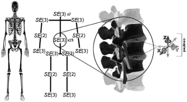
Figure 2: The configuration manifold $M_{hum}$ of the human body is defined as a topological product of constrained $SE(3)$ groups acting in all major (synovial) human joints, $M_{hum}=\prod_{i}SE(3)^{i}$.

Briefly, the Euclidean SE(3)–group is defined as a semidirect (noncommutative) product of 3D rotations and 3D translations, $SE(3):=SO(3)\rhd\mathbb{R}^{3}$. Its most important subgroups are the following [GaneshSprBig, 12, 9]):

4.2 Time–Dependent Biodynamics

Recall that in ordinary autonomous mechanics we have a configuration manifold $M$ (which denotes both $M_{rob}$ and $M_{hum}$), coordinated by $(x^{i})$, and the corresponding velocity phase–space manifold is its tangent bundle $TM$, coordinated by $(x^{i},\dot{x}^{i})$. However, in modern geometrical settings of non–autonomous mechanics, the configuration manifold of time–dependent mechanics is a fibre bundle $\pi:M\rightarrow\mathbb{R}$, called the configuration bundle, coordinated by $(t,x^{i})$, where $t\in\mathbb{R}$ is a Cartesian coordinate on the time axis $\mathbb{R}$ with the transition functions $t{{}^{\prime}}=t+$const. The corresponding velocity phase–space is the 1–jet space $J^{1}(\mathbb{R},M)$, which admits the adapted coordinates $(t,x^{i},x^{i}_{t})=(t,x^{i},\dot{x}^{i})$. Every dynamical equation $\xi$ defines a connection on the affine jet bundle $J^{1}(\mathbb{R},M)\rightarrow M$, and vice versa [9].

Given the configuration fibre bundle $M\rightarrow\mathbb{R}$ over the time axis $\mathbb{R}$, we say that the $1-$jet manifold $J^{1}(\mathbb{R},M)$ is defined as the set of equivalence classes $j_{t}^{1}s$ of sections $s^{i}:\mathbb{R}\rightarrow M$ of the bundle $M\rightarrow\mathbb{R}$, which are identified by their values $s^{i}(t)$, as well as by the values of their partial derivatives $\partial_{t}s^{i}=\partial_{t}s^{i}(t)$ at time points $t\in\mathbb{R}$. The 1–jet manifold $J^{1}(\mathbb{R},M)$ is coordinated by $(t,x^{i},\dot{x}^{i})$, so the 1–jets are local coordinate maps

$$j_{t}^{1}s:\mathbb{R}\rightarrow M,~{}t\mapsto(t,x^{i},\dot{x}^{i}).$$

Similarly, the $2-$jet manifold $J^{2}(\mathbb{R},M)$ is the set of equivalence classes $j_{t}^{2}s$ of sections $s^{i}:\mathbb{R}\rightarrow M$ of the configuration bundle $\pi:M\rightarrow\mathbb{R}$, which are identified by their values $s^{i}(t)$, as well as the values of their first and second partial derivatives, $\partial_{t}s^{i}=\partial_{t}s^{i}(t)$ and $\partial_{tt}s^{i}=\partial_{tt}s^{i}(t)$, respectively, at time points $t\in\mathbb{R}$. The 2–jet manifold $J^{2}(\mathbb{R},M)$ is coordinated by $(t,x^{i},\dot{x}^{i},\ddot{x}^{i})$, so the 2–jets are local coordinate maps

$$j_{t}^{2}s:\mathbb{R}\rightarrow M,~{}t\mapsto(t,x^{i},\dot{x}^{i},\ddot{x}^{i}).$$

Given the configuration bundle $M\rightarrow\mathbb{R}$, coordinated by $(t,x^{i})$, and its 2–jet space $J^{2}(\mathbb{R},M)$, coordinated by $(t,x^{i},x_{t}^{i},x_{tt}^{i})$, any dynamical equation $\xi$ on the configuration bundle $M\rightarrow\mathbb{R}$, which generalizes Lagrangian equation (6),

$$\xi:\quad x_{tt}^{i}=\xi^{i}(t,x^{i},x_{t}^{i})$$ (19)

is equivalent to the geodesic equation with respect to some affine connection $\Gamma$ on the tangent bundle $TM\rightarrow M$,

$$\dot{t}=1,\qquad\ddot{t}=0,\qquad\,\ddot{x}^{i}=\Gamma_{0}^{i}+\Gamma_{j}^{i}\dot{x}^{j},$$

which fulfills the conditions

$$\Gamma_{\alpha}^{0}=0,\qquad\xi^{i}=\Gamma_{0}^{i}+x_{t}^{j}\Gamma_{j}^{i}\mid_{\dot{t}=1,\dot{x}^{i}=x_{t}^{i}}.$$ (20)

A holonomic connection $\xi$ is represented by the horizontal vector–field on $J^{1}(\mathbb{R},M)$,

$$\xi=\partial_{t}+x_{t}^{i}\partial_{i}+\xi^{i}(x^{\mu},x_{t}^{i})\partial_{i}^{t}.$$ (21)

A dynamical equation $\xi$ is said to be conservative if there exists a trivialization $M\cong\mathbb{R}\times M$ such that the vector–field $\xi$ (21) on $J^{1}(\mathbb{R},M)\cong\mathbb{R}\times TM$ is projectable onto $TM$. Then this projection

$$\Xi_{\xi}=\dot{x}^{i}\partial_{i}+\xi^{i}(x^{j},\dot{x}^{j})\dot{\partial}_{i}$$

is a second–order dynamical equation on a typical fibre $M$ of $M\rightarrow\mathbb{R}$,

$$\ddot{x}^{i}=\Xi_{\xi}^{i}.$$ (22)

Conversely, every second–order dynamical equation $\Xi$ (22) on a manifold $M$ can be seen as a conservative dynamical equation

$$\xi_{\Xi}=\partial_{t}+\dot{x}^{i}\partial_{i}+u^{i}\dot{\partial}_{i}$$

on the trivial fibre bundle $\mathbb{R}\times M\rightarrow\mathbb{R}$.

4.2.1 Nonautonomous Dissipative Hamiltonian Dynamics

We can now formulate the time-dependent biomechanics [13, 14, 15] in which the biomechanical phase space is the Legendre manifold $\Pi$, endowed with the holonomic coordinates $(t,y^{i},p_{i})$ with the transition functions

$$p_{i}^{\prime}=\frac{\partial y^{j}}{\partial{y^{\prime}}^{i}}p_{j}.$$

$\Pi$ admits the canonical form ${\Lambda}$ given by

$${\Lambda}=dp_{i}\wedge dy^{i}\wedge dt\otimes\partial_{t}.$$

We say that a connection

$$\gamma=dt\otimes(\partial_{t}+\gamma^{i}\partial_{i}+\gamma_{i}\partial^{i})$$

on the bundle $\Pi\rightarrow X$ is locally Hamiltonian if the exterior form $\gamma\rfloor{\Lambda}$ is closed and Hamiltonian if the form $\gamma\rfloor{\Lambda}$ is exact [16]. A connection $\gamma$ is locally Hamiltonian iff it obeys the conditions:

$$\partial^{i}\gamma^{j}-\partial^{j}\gamma^{i}=0,\quad\partial_{i}\gamma_{j}-\partial_{j}\gamma_{i}=0,\quad\partial_{j}\gamma^{i}+\partial^{i}\gamma_{j}=0.$$

Note that every connection $\Gamma=dt\otimes(\partial_{t}+\Gamma^{i}\partial_{i})$ on the bundle $Y\allowbreak\mathrel{\mathop{\hbox to11.99998pt{\rightarrowfill}}\limits}X$ gives rise to the Hamiltonian connection $\widetilde{\Gamma}$ on $\Pi\allowbreak\mathrel{\mathop{\hbox to11.99998pt{\rightarrowfill}}\limits}X$, given by

$$\widetilde{\Gamma}=dt\otimes(\partial_{t}+\Gamma^{i}\partial_{i}-\partial_{j}\Gamma^{i}p_{i}\partial^{j}).$$

The corresponding Hamiltonian form $H_{\Gamma}$ is given by

$$H_{\Gamma}=p_{i}dy^{i}-p_{i}\Gamma^{i}dt.$$

Let $H$ be a dissipative Hamiltonian form on $\Pi$, which reads:

$$H=p_{i}dy^{i}-\mathcal{H}dt=p_{i}dy^{i}-p_{i}\Gamma^{i}dt-\widetilde{\mathcal{H}}_{\Gamma}dt.$$ (23)

We call $\mathcal{H}$ and $\widetilde{\mathcal{H}}$ in the decomposition (23) the Hamiltonian and the Hamiltonian function respectively. Let $\gamma$ be a Hamiltonian connection on $\Pi\allowbreak\mathrel{\mathop{\hbox to11.99998pt{\rightarrowfill}}\limits}X$ associated with the Hamiltonian form (23). It satisfies the relations [16]

$$\gamma\rfloor{\Lambda}=dp_{i}\wedge dy^{i}+\gamma_{i}dy^{i}\wedge dt-\gamma^{i}dp_{i}\wedge dt=dH,$$

$$\gamma^{i}=\partial^{i}\mathcal{H},\qquad\gamma_{i}=-\partial_{i}\mathcal{H}.$$ (24)

From equations (24) we see that, in the case of biomechanics, one and only one Hamiltonian connection is associated with a given Hamiltonian form.

Every connection $\gamma$ on $\Pi\allowbreak\mathrel{\mathop{\hbox to11.99998pt{\rightarrowfill}}\limits}X$ yields the system of first–order differential equations:

$$\dot{y}^{i}=\gamma^{i},\qquad\dot{p}_{i}=\gamma_{i}.$$ (25)

They are called the evolution equations. If $\gamma$ is a Hamiltonian connection associated with the Hamiltonian form $H$ (23), the evolution equations (25) become the dissipative time-dependent Hamiltonian equations:

$$\dot{y}^{i}=\partial^{i}\mathcal{H},\qquad\dot{p}_{i}=-\partial_{i}\mathcal{H}.$$ (26)

In addition, given any scalar function $f$ on $\Pi$, we have the dissipative Hamiltonian evolution equation

$$d_{H}f=(\partial_{t}+\partial^{i}\mathcal{H}\partial_{i}-\partial_{i}\mathcal{H}\partial^{i})\,f,$$ (27)

relative to the Hamiltonian $\mathcal{H}$. On solutions $s$ of the Hamiltonian equations (26), the evolution equation (27) is equal to the total time derivative of the function $f$:

$$s^{*}d_{H}f=\frac{d}{dt}(f\circ s).$$

4.2.2 Neuro–Muscular Fitness Dynamics

The dissipative Hamiltonian system (26)–(27) is the basis for our time & fitness-dependent biomechanics. The scalar function $f$ in (27) on the biomechanical Legendre phase-space manifold $\Pi$ is now interpreted as an individual neuro-muscular fitness function. This fitness function is a ‘determinant’ for the performance of muscular drives for the driven, dissipative Hamiltonian biomechanics. These muscular drives, for all active DOF, are given by time & fitness-dependent Pfaffian form: $F_{i}=F_{i}(t,y,p,f)$. In this way, we obtain our final model for time & fitness-dependent Hamiltonian biomechanics:

$$\dot{y}^{i} = \partial^{i}\mathcal{H},$$

$$\dot{p}_{i} = F_{i}-\partial_{i}\mathcal{H},$$

$$d_{H}f = (\partial_{t}+\partial^{i}\mathcal{H}\partial_{i}-\partial_{i}\mathcal{H}\partial^{i})\,f.$$

Physiologically, the active muscular drives $F_{i}=F_{i}(t,y,p,f)$ consist of [2]):

1. Synovial joint mechanics, giving the first stabilizing effect to the conservative skeleton dynamics, is described by the $(y,\dot{y})$–form of the Rayleigh–Van der Pol’s dissipation function

$$R=\frac{1}{2}\sum_{i=1}^{n}\,(\dot{y}^{i})^{2}\,[\alpha_{i}\,+\,\beta_{i}(y^{i})^{2}],\quad$$

where $\alpha_{i}$ and $\beta_{i}$ denote dissipation parameters. Its partial derivatives give rise to the viscous–damping torques and forces in the joints

$$\mathcal{F}_{i}^{joint}=\partial R/\partial\dot{y}^{i},$$

which are linear in $\dot{y}^{i}$ and quadratic in $y^{i}$.

2. Muscular mechanics, giving the driving torques and forces $\mathcal{F}_{i}^{musc}=\mathcal{F}_{i}^{musc}(t,y,\dot{y})$ with $(i=1,\dots,n)$ for human biomechanics, describes the internal excitation and contraction dynamics of equivalent muscular actuators [2].

(a) The excitation dynamics can be described by an impulse force–time relation

$$F_{i}^{imp} = F_{i}^{0}(1\,-\,e^{-t/\tau_{i}})\text{ \qquad if stimulation }>0$$

$$\quad F_{i}^{imp} = F_{i}^{0}e^{-t/\tau_{i}}\qquad\qquad\;\quad\text{if stimulation }=0,\quad$$

where $F_{i}^{0}$ denote the maximal isometric muscular torques and forces, while $\tau_{i}$ denote the associated time characteristics of particular muscular actuators. This relation represents a solution of the Wilkie’s muscular active–state element equation [17]

$$\dot{\mu}\,+\,\Gamma\,\mu\,=\,\Gamma\,S\,A,\quad\mu(0)\,=\,0,\quad 0<S<1,$$

where $\mu=\mu(t)$ represents the active state of the muscle, $\Gamma$ denotes the element gain, $A$ corresponds to the maximum tension the element can develop, and $S=S(r)$ is the ‘desired’ active state as a function of the motor unit stimulus rate $r$. This is the basis for biomechanical force controller.

(b) The contraction dynamics has classically been described by Hill’s hyperbolic force–velocity relation [18]

$$F_{i}^{Hill}\,=\,\frac{\left(F_{i}^{0}b_{i}\,-\,\delta_{ij}a_{i}\dot{y}^{j}\,\right)}{\left(\delta_{ij}\dot{y}^{j}\,+\,b_{i}\right)},\,\quad$$

where $a_{i}$ and $b_{i}$ denote Hill’s parameters, corresponding to the energy dissipated during the contraction and the phosphagenic energy conversion rate, respectively, while $\delta_{ij}$ is the Kronecker’s $\delta-$tensor.

In this way, human biomechanics describes the excitation/contraction dynamics for the $i$th equivalent muscle–joint actuator, using the simple impulse–hyperbolic product relation

$$\mathcal{F}_{i}^{musc}(t,y,\dot{y})=\,F_{i}^{imp}\times F_{i}^{Hill}.\quad$$

5 Hierarchical Control of Humanoid Robots

5.1 Spinal Control Level

The force HBE servo–controller is formulated as affine control Hamiltonian–systems (17–18) (with possible extensions along the lines of the previous section), which resemble an autogenetic motor servo [20], acting on the spinal–reflex level of the human locomotion control. A voluntary contraction force $F$ of human skeletal muscle is reflexly excited (positive feedback $+F^{-1}$) by the responses of its spindle receptors to stretch and is reflexly inhibited (negative feedback $-F^{-1}$) by the responses of its Golgi tendon organs to contraction. Stretch and unloading reflexes are mediated by combined actions of several autogenetic neural pathways, forming the so–called $\mathbf{`}$motor servo.’ The term $\mathbf{`}$autogenetic’ means that the stimulus excites receptors located in the same muscle that is the target of the reflex response. The most important of these muscle receptors are the primary and secondary endings in the muscle–spindles, which are sensitive to length change – positive length feedback $+F^{-1}$, and the Golgi tendon organs, which are sensitive to contractile force – negative force feedback $-F^{-1}$.

The gain $G$ of the length feedback $+F^{-1}$ can be expressed as the positional stiffness (the ratio $G\approx S=dF/dx$ of the force–$F$ change to the length–$x$ change) of the muscle system. The greater the stiffness $S$, the less the muscle will be disturbed by a change in load. The autogenetic circuits $+F^{-1}$ and $-F^{-1}$ appear to function as servoregulatory loops that convey continuously graded amounts of excitation and inhibition to the large (alpha) skeletomotor neurons. Small (gamma) fusimotor neurons innervate the contractile poles of muscle spindles and function to modulate spindle–receptor discharge.

5.2 Cerebellum–Like Velocity and Jerk Control

Nonlinear velocity and jerk (time derivative of acceleration) servo–controllers [2], developed using the Lie–derivative formalism [1], resemble self–stabilizing and adaptive tracking action of the cerebellum [21]. By introducing the vector–fields $f$ and $g$, given respectively by

$$f=\left(\partial_{p_{i}}H_{0},\,-\partial_{q^{i}}H_{0}\right),\qquad g=\left(-\partial_{p_{i}}H^{j},\,\partial_{q^{i}}H^{j}\right),$$

we obtain the affine controller in the standard nonlinear MIMO–system form (see [9])

$$\dot{x}_{i}=f(x)+g(x)\,u_{j}.$$ (28)

Finally, using the Lie derivative formalism [9] and applying the constant relative degree $r$ to all HB joints, the control law for asymptotic tracking of the reference outputs $o_{R}^{j}=o_{R}^{j}(t)$ could be formulated as (generalized from [22])

$$u_{j}=\frac{\dot{o}_{R}^{(r)j}-L_{f}^{(r)}H^{j}+\sum_{s=1}^{r}c_{s-1}(o_{R}^{(s-1)j}-L_{f}^{(s-1)}H^{j})}{L_{g}L_{f}^{(r-1)}H^{j}},$$ (29)

where $c_{s-1}$ are the coefficients of the linear differential equation of order $r$ for the error function $e(t)=x^{j}(t)-o_{R}^{j}(t)$

$$e^{(r)}+c_{r-1}e^{(r-1)}+\dots+c_{1}e^{(1)}+c_{0}e=0.$$

The control law (29) can be implemented symbolically in $Mathematica^{TM}$ in the following three steps:

1. Symbolic functions defining the gradient and Lie derivatives:

$$\text{Grad}[s\_,x\_\text{List}] : =(D[s,\#1]\&)/@x;$$

$$\text{LieDer}[v\_\text{List},s\_,x\_\text{List}] : =\text{Grad}[s,x]\cdot v;$$

$$\text{KLieDer}[v\_\text{List},s\_,x\_\text{List},k\_] : =$$

$$\text{Block}[\{t\},p : =s;~{}\text{If}[k==0,p=s,\text{Do}[p=\text{LieDer}[v,p,x],\{k\}]];p];$$

2. Control law defined (for simplicity, we show here only the first–order control law):

$$u[t\_]=(-\text{LieDer}[F,y,X]+D[yR[t],t]+\alpha(yR[t]-y))/\text{LieDer}[g,y,X];$$

3. Example for the reference output $yR[t],$ with the final time Tfin:

$$yR[t\_]=\text{If}[t<=\text{Tfin}/2,5(1-\text{e}^{-5t}),(5(1-\text{e}^{-5t}))/\text{e}^{(5(t-\text{Tfin}/2)})];$$

The affine nonlinear MIMO control system (28) with the Lie–derivative control law (29) resembles the self–stabilizing and synergistic output tracking action of the human cerebellum [24]. To make it adaptive (and thus more realistic), instead of the ‘rigid’ controller (29), we can use the adaptive Lie–derivative controller, as explained in the seminal paper on geometrical nonlinear control [23].

5.3 Cortical–Like Fuzzy–Topological Control

For the purpose of our cortical control, the dominant, rotational part of the human configuration manifold $M^{N}$, could be first, reduced to an $N$–torus, and second, transformed to an $N$–cube (‘hyper–joystick’), using the following topological techniques (see [9]).

Let $S^{1}$ denote the constrained unit circle in the complex plane, which is an Abelian Lie group. Firstly, we propose two reduction homeomorphisms, using the Cartesian product of the constrained $SO(2)-$groups:

$$SO(3)\approx SO(2)\times SO(2)\times SO(2)\qquad\text{and}\qquad SO(2)\approx S^{1}.$$

Next, let $I^{N}$ be the unit cube $[0,1]^{N}$ in $\mathbb{R}^{N}$ and ‘$\sim$’ an equivalence relation on $\mathbb{R}^{N}$ obtained by ‘gluing’ together the opposite sides of $I^{N}$, preserving their orientation. Therefore, $M^{N}$ can be represented as the quotient space of $\mathbb{R}^{N}$ by the space of the integral lattice points in $\mathbb{R}^{N}$, that is an oriented and constrained $N$–dimensional torus $T^{N}$:

$${\mathbb{R}^{N}/{Z}^{N}}\approx\,\prod_{i=1}^{N}S_{i}^{1}\equiv\{(q^{i},\,i=1,\dots,N):\mbox{mod}2\pi\}=T^{N}.$$ (30)

Its Euler–Poincaré characteristic is (by the De Rham theorem) both for the configuration manifold $T^{N}$ and its momentum phase–space $T^{\ast}T^{N}$ given by (see [9])

$$\chi(T^{N},T^{\ast}T^{N})=\sum_{p=1}^{N}(-1)^{p}b_{p}\,,$$

where $b_{p}$ are the Betti numbers defined as

$$b^{0} =1,\,$$

$$b^{1} =N,\dots b^{p}={\binom{N}{p}},\dots b^{N-1}=N,$$

$$b^{N} =1,\qquad\qquad(0\leq p\leq N).$$

Conversely by ‘ungluing’ the configuration space we obtain the primary unit cube. Let ‘$\sim^{\ast}$’ denote an equivalent decomposition or ‘ungluing’ relation. According to Tychonoff’s product–topology theorem [9], for every such quotient space there exists a ‘selector’ such that their quotient models are homeomorphic, that is, $T^{N}/\sim^{\ast}\approx A^{N}/\sim^{\ast}$. Therefore $I_{q}^{N}$ represents a ‘selector’ for the configuration torus $T^{N}$ and can be used as an $N$–directional ‘$\hat{q}$–command–space’ for the feedback control (FC). Any subset of degrees of freedom on the configuration torus $T^{N}$ representing the joints included in HB has its simple, rectangular image in the rectified $\hat{q}$–command space – selector $I_{q}^{N}$, and any joint angle $q^{i}$ has its rectified image $\hat{q}^{i}$.

In the case of an end–effector, $\hat{q}^{i}$ reduces to the position vector in external–Cartesian coordinates $z^{r}\,(r=1,\dots,3)$. If orientation of the end–effector can be neglected, this gives a topological solution to the standard inverse kinematics problem.

Analogously, all momenta $\hat{p}_{i}$ have their images as rectified momenta $\hat{p}_{i}$ in the $\hat{p}$–command space – selector $I_{p}^{N}$. Therefore, the total momentum phase–space manifold $T^{\ast}T^{N}$ obtains its ‘cortical image’ as the $\widehat{(q,p)}$–command space, a trivial $2N$–dimensional bundle $I_{q}^{N}\times I_{p}^{N}$.

Now, the simplest way to perform the feedback FC on the cortical $\widehat{(q,p)}$–command space $I_{q}^{N}\times I_{p}^{N}$, and also to mimic the cortical–like behavior, is to use the $2N$– dimensional fuzzy–logic controller, in much the same way as in the popular ‘inverted pendulum’ examples (see [19]).

We propose the fuzzy feedback–control map $\Xi$ that maps all the rectified joint angles and momenta into the feedback–control one–forms

$$\Xi:(\hat{q}^{i}(t),\,\hat{p}_{i}(t))\mapsto u_{i}(t,q,p),$$ (31)

so that their corresponding universes of discourse, $\hat{Q}^{i}=(\hat{q}_{max}^{i}-\hat{q}_{min}^{i})$, $\hat{P}_{i}=(\hat{p}_{i}^{max}-\hat{p}_{i}^{min})$ and $\hat{U}{}_{i}=(u_{i}^{max}-u_{i}^{min})$, respectively, are mapped as

$$\Xi:\prod_{i=1}^{N}\hat{Q}^{i}\times\prod_{i=1}^{N}\hat{P}_{i}\rightarrow\prod_{i=1}^{N}{}\hat{U}{}_{i}.$$ (32)

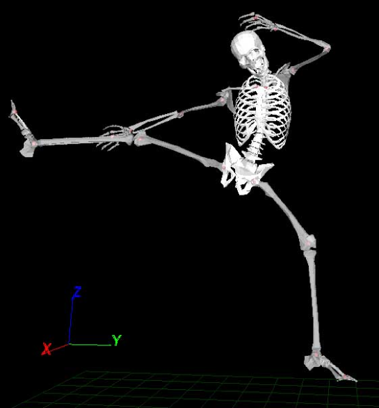
Figure 3: The HBE simulating a jump-kick: a 3D viewer.

The $2N$–dimensional map $\Xi$ (31,32) represents a fuzzy inference system, defined by [24]:

1. Fuzzification of the crisp rectified and discretized angles, momenta and controls using Gaussian–bell membership functions

   $$\mu_{k}(\chi)=\exp[-\frac{(\chi-m_{k})^{2}}{2\sigma_{k}}],\qquad(k=1,2,\dots,9),$$

   where $\chi\in D$ is the common symbol for $\hat{q}^{i}$, $\hat{p}_{i}$ and $u_{i}(q,p)$ and $D$ is the common symbol for $\hat{Q}^{i},\hat{P}_{i}$ and _i; the mean values $m_{k}$ of the nine partitions of each universe of discourse $D$ are defined as $m_{k}=\lambda_{k}D+\chi_{min}$, with partition coefficients $\lambda_{k}$ uniformly spanning the range of $D$, corresponding to the set of nine linguistic variables $L=\{NL,NB,NM,NS,ZE,PS,PM$, $PB,PL\}$; standard deviations are kept constant $\sigma_{k}=D/9$. Using the linguistic vector $L$, the $9\times 9$ FAM (fuzzy associative memory) matrix (a ‘linguistic phase–plane’), is heuristically defined for each human joint, in a symmetrical weighted form

   $$\mu_{kl}=\varpi_{kl}\,exp\{-50[\lambda_{k}+u(q,p)]^{2}\},\qquad(k,l=1,...,9)$$

   with weights $\varpi_{kl}\in\{0.6,0.6,0.7,0.7,0.8,0.8,0.9,0.9,1.0\}$.

2. Mamdani inference is used on each FAM–matrix $\mu_{kl}$ for all human joints:
   (i) $\mu(\hat{q}^{i})$ and $\mu(\hat{p}_{i})$ are combined inside the fuzzy IF–THEN rules using AND (Intersection, or Minimum) operator,

   $$\mu_{k}[\bar{u}_{i}(q,p)]=\min_{l}\{\mu_{kl}(\hat{q}^{i}),\,\mu_{kl}(\hat{p}_{i})\}.$$

   (ii) the output sets from different IF–THEN rules are then combined using OR (Union, or Maximum) operator, to get the final output, fuzzy–covariant torques,

   $$\mu[u_{i}(q,p)]=\max_{k}\{\mu_{k}[\bar{u}_{i}(q,p)]\}.$$

3. Defuzzification of the fuzzy controls $\mu[u_{i}(q,p)]$ with the ‘center of gravity’ method

   $$u_{i}(q,p)=\frac{\int\mu[u_{i}(q,p)]\,du_{i}}{\int du_{i}},$$

   to update the crisp feedback–control one–forms $u_{i}=u_{i}(t,q,p)$.

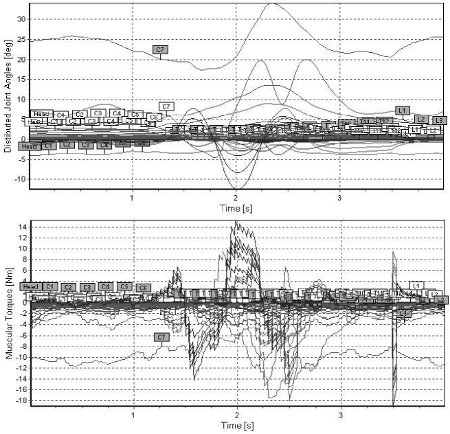
Figure 4: The HBE simulating a jump-kick: calculating joint angles and muscular torques.

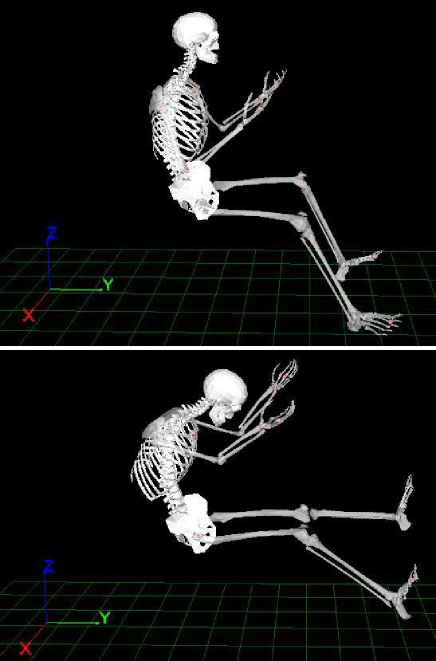
Figure 5: The HBE simulating the frontal road-vehicle crash into the fixed wall with a speed of 70 km/h: before the impact (up) and 0.12 s after the impact.

Now, it is easy to make this top–level controller adaptive, simply by weighting both the above fuzzy–rules and membership functions, by the use of any standard competitive neural–network (see, e.g., [19]). Operationally, the construction of the cortical $\widehat{(q,p)}$–command space $I_{q}^{N}\times I_{p}^{N}$ and the $2N$–dimensional feedback map $\Xi$ (31,32), mimic the regulation of the motor conditioned reflexes by the motor cortex [21].

It has been implicitly assumed that close resemblance of hierarchical control structures presented in this section with the corresponding human neuro-physiological control mechanisms would assure the necessary overall stability of biodynamics. However, in future work, these control structures need to be properly analyzed, starting with Lyapunov stability criteria.

6 Simulation Examples

In this section we give several simulation examples of the sophisticated virtual humanoid called Human Biodynamics Engine (HBE), designed at Defence Science & Technology Organisation, Australia. The HBE is a sophisticated human neuro-musculo-skeletal dynamics simulator, based on generalized Lagrangian and Hamiltonian mechanics and Lie-derivative nonlinear control. It includes 270 active degrees of freedom (DOF), while fingers are not separately modelled: 135 rotational DOF are considered active, and 135 translational DOF are considered passive. The HBE incorporates both forward and inverse dynamics, as well as two neural–like control levels. Active rotational joint dynamics is driven by 270 nonlinear muscular actuators, each with its own excitation–contraction dynamics (following traditional Hill–Hatze biomechanical models). Passive translational joint dynamics models visco-elastic properties of inter-vertebral discs, joint tendons and muscular ligaments as a nonlinear spring-damper system. The lower neural control level resembles spinal–reflex positive and negative force feedbacks, resembling stretch and Golgi reflexes, respectively. The higher neural control level mimics cerebellum postural stabilization and velocity target-tracking control. The HBE’s core is the full spine simulator, considering human spine as a chain of 26 flexibly–coupled rigid bodies (formally, the product of 26 SE(3)–groups). The HBE includes over 3000 body parameters, all derived from individual user data, using standard biomechanical tables. The HBE incorporates a new theory of soft neuro-musculo-skeletal injuries, based on the concept of the local rotational and translational jolts, which are the time rates of change of the total forces and torques localized in each joint at a particular time instant.

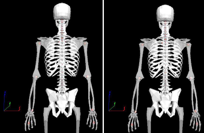
Figure 6: The HBE simulating an effect of an aircraft pilot-seat ejection to human spine compression: before the seat ejection (left) and after ejection (right).

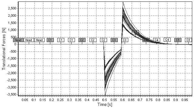
Figure 7: The HBE calculating translational forces distributed along the spinal joints during the seat ejection.

The first version of the HBE simulator had the full human-like skeleton, driven by the generalized Hamiltonian dynamics (including muscular force-velocity and force-time curves) and two levels of reflex-like motor control (simulated using the Lie derivative formalism) [1, 2]. It had 135 purely rotational DOF, strictly following Figure 1. It was created for prediction and prevention of musculo-skeletal injuries occurring in the joints, mostly spinal (intervertebral). Its performance looked kinematically realistic, while it was not possible to validate the driving torques. It included a small library of target movements which were followed by the HBE’s Lie–derivative controllers with efficiency of about 90% (see Figures 3 and 4).

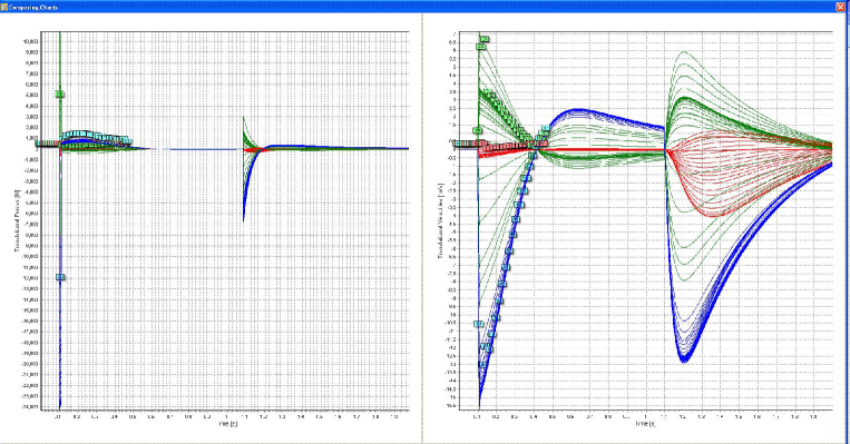
Figure 8: The HBE simulating a double-impact effect of a land-mine blast under an armor-protected vehicle to a hypothetical passenger’s body.

The HBE also includes a generic crash simulator, based on the simplified road-vehicle impact simulator (see Figure 5). While implementing the generic crash simulator, it became clear that purely rotational joint dynamics would not be sufficient for the realistic prediction of musculo-skeletal injuries. In particular, to simulate the action of a Russian aircraft ejection-seat currently used by the American space shuttle, we needed to implement micro translations in the intervertebral joints (see Figures 6 and 7). This is because the seat provides full body restraint and hence the ejection rockets firing with 15 g per .15 s cause pure compression of the spine (without any bending).

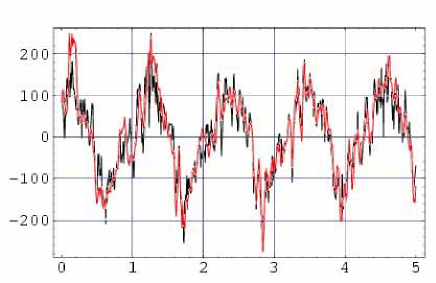
Figure 9: Matching the ‘Vicon’ output with the ‘HBE’ output for the right-hip angular velocity around the dominant X-axis, while walking on a treadmill with a speed of 4 km/h.

Finally, the HBE includes the defence-specific land-mine crash simulator. It is calibrated on a hypothetical double-impact under the armor-protected military vehicle, including:

1. A land-mine blast of 350g with a duration of 5ms;

2. A 1s pause when the hypothetical vehicle is in the air;  and

3. The vehicle hard landing with an acceleration of 100g and a duration 1s.

The HBE calculates full rotational and translational dynamics caused by the land-mine double-impact in extreme force/time scales (including both linear and angular displacements, velocities, forces and jolts in all human joints (see Figure 8)). The variations of the applied g-forces and durations of the two impacts can be simulated, to see the differences in their effects on the hypothetical passenger’s body.

In this way a full rotational + translational biodynamics simulator has been created with 270 DOF in total (not representing separate fingers). The ‘HBE-simulator’ has been kinematically validated (see Figure 9) against the standard biomechanical gait-analysis system ‘Vicon’ [25].

References

• [1] Ivancevic, V. Symplectic Rotational Geometry in Human Biomechanics. SIAM Rev. 46(3), 455–474 (2004).
• [2] Ivancevic, V., Ivancevic, T., Human-Like Biomechanics: A Unified Mathematical Approach to Human Biomechanics and Humanoid Robotics. Springer, Berlin, (2005).
• [3] Ivancevic, V., Sharma, S., Complexity in Human Bio-Mechanics. IJHR, 5(4), 679–698 (2008)
• [4] V. Ivancevic and T. Ivancevic, Human versus Humanoid Biodynamics, IJHR, 5(4), 699–713, (2008).
• [5] Arnold, V.I., Mathematical Methods of Classical Mechanics. Springer, New York, (1978).
• [6] Abraham, R., Marsden, J., Foundations of Mechanics. Benjamin, Reading, MA, (1978).
• [7] Marsden, J.E., Ratiu, T.S., Introduction to Mechanics and Symmetry: A Basic Exposition of Classical Mechanical Systems. (2nd ed), Springer, New York, (1999).
• [8] Ivancevic, V., LieLagrangian model for realistic human biodynamics. IJHR, 3(2), 205-218 (2006).
• [9] Ivancevic, V., Ivancevic, T., Applied Differential Geometry: A Modern Introduction. World Scientific, Singapore, (2007).
• [10] Ivancevic, V., Generalized Hamiltonian Biodynamics and Topology Invariants of Humanoid Robots, IJMMS, 31(9), 555-565 (2002).
• [11] Ivancevic, V., Beagley, N. Brain-like functor control machine for general humanoid biodynamics, IJMMS, 11, 1759-1779 (2005).
• [12] Park, J., Chung, W.-K. Geometric Integration on Euclidean Group With Application to Articulated Multibody Systems. IEEE Trans. Rob. 21(5), 850–863 (2005).
• [13] Ivancevic, T., Jet Methods in Time–Dependent Lagrangian Biomechanics, Cent. Eur. J. Phys. 8(5), (2010).
• [14] Ivancevic, T. et al, Jet spaces in modern Hamiltonian biomechanics, Cent. Eur. J. Phys. 8(6), (2010).
• [15] Ivancevic, T., Jet–Ricci Geometry of Time-Dependent Human Biomechanics, Int. J. Biomath. 3(1), 1–13, (2010).
• [16] Giachetta, G., Mangiarotti, L., Sardanashvily, G., New Lagrangian and Hamiltonian Methods in Field Theory, World Scientific, Singapore, (1997)
• [17] Wilkie, D.R., The mechanical properties of muscle. Brit. Med. Bull. 12, 177–182, (1956)
• [18] Hill, A.V.,The heat of shortening and the dynamic constants of muscle. Proc. Roy. Soc. B76, 136–195, (1938)
• [19] Kosko, B., Neural Networks and Fuzzy Systems, A Dynamical Systems Approach to Machine Intelligence. Prentice–Hall, New York, (1992)
• [20] Houk, J.C., Regulation of stiffness by skeletomotor reflexes. Ann. Rev. Physiol. 41, 99-123, (1979)
• [21] Houk, J.C., Buckingham, J.T., Barto, A.G., Models of the cerebellum and motor learning. Beh. Brain Sci. 19(3), 368–383, (1996)
• [22] Isidori, A., Nonlinear Control Systems, An Introduction (2nd ed.) Springer, Berlin, (1989)
• [23] Sastri, S.S., Isidori, A., Adaptive control of linearizable systems, IEEE Trans. Aut. Con. 34(11), 1123–1131, (1989)
• [24] Ivancevic, V., Ivancevic, T., Neuro–Fuzzy Associative Machinery for Comprehensive Brain and Cognition Modelling. Springer, Berlin, (2007)
• [25] Robertson, D.G.E., Caldwell, G.H., Hamill, J., Kamen,G., Whittlesey, S.N., Research Methods in Biomechanics. Human Kinetics, Champaign, IL, (2004)