Fluctuations of two-time quantities and time-reparametrization invariance in spin-glasses

Abstract

This article is a contribution to the understanding of fluctuations in the out of equilibrium dynamics of glassy systems. By extending theoretical ideas based on the assumption that time-reparametrization invariance develops asymptotically we deduce the scaling properties of diverse high-order correlation functions. We examine these predictions with numerical tests in a standard glassy model, the $3d$ Edwards-Anderson spin-glass, and in a system where time-reparametrization invariance is not expected to hold, the $2d$ ferromagnetic Ising model, both at low temperatures. Our results enlighten a qualitative difference between the fluctuation properties of the two models and show that scaling properties conform to the time-reparametrization invariance scenario in the former but not in the latter.

PACS: 05.70.Ln, 75.40.Gb, 05.40.-a

I Introduction

In a series of papers the idea that time-reparametrization invariance (TRI) should be the reason for large non-equilibrium fluctuations in glassy systems was introduced. This claim was substantiated with the analysis of the Martin-Siggia-Rose-Janssen-deDominicis (MSRJD) action for Langevin stochastic processes Chamon02 ; Castillo02 ; Charbonneau04 ; Castillo2 and by numerical simulations of various glassy models Castillo02 ; Charbonneau04 ; Jaubert07 ; Castillo3 . The state of the art of these ideas is summarized in Chamon07 .

The non-equilibrium situation we are concerned with is a dynamic process where a system is quenched below a transition or dynamic crossover with some protocol and it is let relax subsequently. The most interesting time regime after the quench is the one in which the size of the sample is the largest (though still finite) scale and times are long but not as much as to allow for equilibration. The system is then in an asymptotic non-equilibrium regime in which a kind of dynamic scaling is very often realized. In this stage the behavior of time-dependent observables is rather well understood reviews-mean-field .

The sources of fluctuations in the dynamics of these systems are disorder in the initial conditions, thermal noise, quenched disorder and external forces, if present. In Chamon07 and references therein the proposal was to average over any sort of quenched randomness with the purpose of bringing together disordered systems – such as spin-glasses, superconductors, or other – and conventional glasses – of atomic, molecular or other nature. External forces were set to zero and had no effect on the dynamics. One is then left with initial condition and thermally induced fluctuations only. In order to study their effects, beside the fully averaged value $X$ of physical quantities, one has to consider the properties of their fluctuating parts $\widehat{X}$, to be defined properly, which may be sample dependent. The most complete characterization of fluctuations is then obtained through the probability distribution $P(\widehat{X})$. In particular, since the relevance of fully-averaged two-time quantities such as the self-correlation $C(t_{1},t_{2})$ function, the linear autoresponse $\chi(t_{1},t_{2})$ and their fluctuating parts, to the issue of TRI was underlined in Chamon02 ; Castillo02 ; ChaCugYos06 , one is interested in the probability distributions of $\widehat{C}$ and $\widehat{\chi}$ studied as a function of $\widehat{C}$, $t_{1}$, $t_{2}$, the system size and the other parameters in the model. This is, however, a formidable task. Less ambitious but still very instructive is to analyze the first moments of the distributions, such as the generalized variances that we shall define in the body of this paper. This is, indeed, the route that we shall follow in this article. Resorting to a Langevin description, in Sec. II we set the formalism for continuous variables systems and then present analytic expressions for these variances in terms of the MSRJD fields, deriving scaling laws based upon the TRI scenario. Next, recalling previous results on linear and beyond-linear response theory CorLipSarZan10f ; LipCorSarZan08 ; LipCorZan05 , we relate these variances to quantities that can be measured in Ising spin systems in Sec. III. In Sec. IV we put the TRI predictions to the test in the Edwards-Anderson (EA) model in $d=3$ by means of extensive numerical simulations. The results, which refine and extend the analysis performed in Castillo02 , are consistent with the predictions of TRI. In the same section we present another set of numerical simulations performed on a coarsening system, the ferromagnetic Ising model in $d=2$, for which TRI is not expected to hold ChaCugYos06 , showing a different pattern of fluctuations, already at a qualitative level. A summary and the conclusions are contained in Sec. V.

II Formalism for systems with continuous variables and time reparametrization invariance

II.1 Generating functional

The stochastic dynamics of continuous variables in a macroscopic system are usually described with a Markovian Langevin equation with additive white noise. The ensemble of such coupled stochastic equations can be recast into a path-integral called Martin-Siggia-Rose-Jenssen-deDominicis (MSRJD) generating functional that is better adapted for a general type of analysis. This formalism has been reviewed in several publications MSJ so we shall not repeat the construction of the path-integral here. It reads

$${\cal Z}[\eta,i\hat{\eta}]=\int{\cal D}\phi{\cal D}i\hat{\phi}\ e^{-S[\Phi;\eta,\hat{\eta}]}\ P_{IC}[\phi(x,t_{0})]$$ (1)

with

$$S[\Phi;\eta,\hat{\eta}]=\int_{t_{0}}^{\infty}dtdx\left\{i\hat{\phi}(x,t)[\dot{\phi}(x,t)+\frac{\delta V[\phi]}{\delta\phi(x,t)}-h(x,t)]+T(i\hat{\phi}(x,t))^{2}+\eta(x,t)\phi(x,t)+\hat{\eta}(x,t)i\hat{\phi}(x,t)\right\}$$ (2)

where, to simplify the notation, we focused on a one-dimensional theory described by a scalar field $\phi$. $t_{0}$ is the initial time, when the system is set in contact with a thermal bath at temperature $T$. We set $k_{B}=1$ and we absorb the friction coefficient into a redefinition of time. $P_{IC}[\phi(x,t_{0})]$ is the probability distribution of the field initial conditions. Henceforth we shall not write the limits of the time-intervals explicitly. $V$ is the potential energy from which the deterministic force in the Langevin equation derives. $h$ is an external perturbation that couples linearly to the field $\phi$ in the potential. $\eta$ and $\hat{\eta}$ are two space and time dependent sources. The path integral runs over all possible configurations of the field $\phi$ with initial condition $\phi(x,t_{0})$. The measure is defined as ${\cal D}\phi\equiv\prod_{k=0}^{\cal N}\prod_{a=1}^{L}d\phi(x_{a},t_{k})$ and we jump over subtle discretization issues that are discussed in many publications by recalling that we do not need to worry about any determinant contribution to the action. The integral over the auxiliary field $i\hat{\phi}(x,t)$ is similarly discretized, namely ${\cal D}i\hat{\phi}\equiv\prod_{k=1}^{\cal N}\prod_{a=1}^{L}di\hat{\phi}(x_{a},t_{k})$. Without loss of generality for our purpose, we take $P_{IC}$ to be flat. We use a compact notation for the two fields, $\Phi=(\phi\;,\;i\hat{\phi})$, in the action and hereafter we label $\Phi^{0}=\phi$ and $\Phi^{1}=i\hat{\phi}$ its components. Due to the normalization of the thermal noise distribution the path-integral is identical to one, ${\cal Z}[0,0]=1$, in the absence of sources; this feature will be useful later. Noise averages translate into averages computed within the path-integral formulation with weight $e^{-S[\Phi;0,0]}$.

For definiteness, and to parallel the discussion in Chamon07 and references therein (to which we refer for further details), let us separate a quadratic term from the non-linear one, $V_{nl}$, in the potential

$$V[\phi]=\frac{1}{2}\int dxdy\ J(x,y)\phi(x,t)\phi(y,t)+V_{nl}[\phi]$$ (3)

and assume that the symmetric time-independent exchange matrix $J$ is made of independent elements each of them Gaussian-distributed $P[J]\propto\prod_{xy}\exp[-(1/2)\int dxdy\ J^{2}(x,y)K^{-1}(x,y)]$ with $K^{-1}$ the connectivity matrix. For a lattice model with first nearest-neighbours and no self-interactions, as the $3d$ Edwards-Anderson spin-glass that we studied numerically, $K^{-1}(x,y)=J^{2}/z$ for nearest-neighbours and zero otherwise, with $J$ the exchange constant and $z$ the connectivity of the lattice. Quenched disorder is treated on average by exploiting the fact that ${\cal Z}[0,0]=1$. Concretely, one averages the dynamic generating functional over the $J$-distribution with no need to use the replica trick. This gives rise to a quartic term in the action of the form

$$S_{4}[\Phi] = -\frac{1}{8}\int dxdy\int dt_{1}dt_{2}\ \left[i\hat{\phi}(x,t_{1})\,\phi(y,t_{1})+\phi(x,t_{1})\,i\hat{\phi}(y,t_{1})\right]K(x,y)\left[i\hat{\phi}(x,t_{2})\,\phi(y,t_{2})+\phi(x,t_{2})\,i\hat{\phi}(y,t_{2})\right]$$ (4)

$$= -\frac{1}{8}\int dxdy\int dt_{1}dt_{2}\ \Phi^{a}(x,t_{1})\Phi^{\bar{a}}(y,t_{1})\,K(x,y)\,\Phi^{b}(x,t_{2})\Phi^{\bar{b}}(y,t_{2}),$$

where $a,b=0,1$ and $\overline{0}=1$ and $\overline{1}=0$ (here repeated indices are summed). This term can be decoupled by introducing four spatially local two-time fields $Q^{ab}(x;t_{1},t_{2})$, $a,b=0,1$, with a Hubbard-Stratonovich transformation. One then has

$$S_{4}[\Phi] = \int{\cal D}Q\exp\left[\frac{1}{2}\int dxdy\ K^{-1}(x,y)\int dt_{1}dt_{2}\ Q^{ab}(x;t_{1},t_{2})Q^{\overline{b}\overline{a}}(y,t_{2},t_{1})\right.$$ (5)

$$\qquad\qquad\qquad\qquad\left.-\int dx\int dt_{1}dt_{2}\ \Phi^{a}(x,t_{1})Q^{ab}(x;t_{1},t_{2})\Phi^{b}(x,t_{2})\right]\;.$$

The zero-source generating functional can now be written as ${\cal Z}[0,0]=\int{\cal D}Q{\cal D}\Phi\ e^{-S[Q,\Phi]}$ where the action $S[Q,\Phi]$ includes all terms, those in Eq. (5) that depend on $Q$ and those in Eq. (2) with $V$ replaced by $V_{nl}$ that depend on $\Phi$ only.

II.2 Relation between composite operators of $Q$ and $\Phi$ fields

The TRI arguments Chamon07 , which are briefly recalled in Sec. II.3, rely on the transformation properties of the fluctuating $Q$ fields that, in turn, translate into relations between the average values of products of the $Q$ fields. These objects, though, are auxiliary in the calculation and are not directly accessible in a simulation or experiment. In order to proceed towards a test of TRI the next step, to which this paragraph is devoted, is to relate the statistical properties of the Hubbard-Stratonovich fields $Q$ to those of the field $\Phi$. In particular, our program is to find relations between averages of products of $Q$s and moments of the $\Phi$s from which directly measurable correlation and response functions will be constructed. To this end we perform an infinitesimal translation of the field $Q\to Q+\delta Q$, which induces a change in the action $S[Q,\Phi]\to S[Q,\Phi]+\delta S[Q,\Phi]$, with

$$\delta S[Q,\Phi] = -\int dx\int dt_{1}dt_{2}\ \Phi^{a}(x,t_{1})\Phi^{b}(x,t_{2})\delta Q^{ab}(x;t_{1},t_{2})+\int dxdy\ K^{-1}(x,y)\int dt_{1}dt_{2}\ \delta Q^{ab}(x;t_{1},t_{2})Q^{\overline{b}\overline{a}}(y,t_{2},t_{1})$$ (6)

$$\qquad\qquad+\frac{1}{2}\int dxdy\ K^{-1}(x,y)\int dt_{1}dt_{2}\ \delta Q^{ab}(x;t_{1},t_{2})\delta Q^{\overline{b}\overline{a}}(y,t_{2},t_{1})\;.$$

The normalization ${\cal Z}[0,0]=1$ implies $\langle e^{-\delta S}\rangle=1$ where $\langle\cdots\rangle=\int{\cal D}\Phi{\cal D}Q\ \cdots\;e^{-S[\Phi,Q]}$. To first and second order in $\delta Q$ one has

$$\int dy\ K^{-1}(x,y)\ \langle Q^{\overline{b}\overline{a}}(y;t_{2},t_{1})\rangle=\langle\Phi^{a}(x,t_{1})\Phi^{b}(x,t_{2})\rangle\;,$$ (7)

and

$$-K^{-1}(x,u)\ \delta_{a\overline{d}}\ \delta_{b\overline{c}}\ \delta(t_{1}-t_{4})\ \delta(t_{2}-t_{3}) = \left\langle\left(\Phi^{a}(x,t_{1})\Phi^{b}(x,t_{2})-\int dy\ K^{-1}(x,y)\ Q^{\overline{b}\overline{a}}(y;t_{2},t_{1})\right)\right.$$ (8)

$$\qquad\times\left.\left(\Phi^{c}(u,t_{3})\Phi^{d}(u,t_{4})-\int dv\ K^{-1}(u,v)\ Q^{\overline{d}\overline{c}}(v;t_{4},t_{3})\right)\right\rangle\;,$$

respectively. The first equation tells us that the average of the Hubbard-Stratonovich $Q$ field, coarse-grained over the region in which $K^{-1}(x,y)$ is different from zero, is equal to the correlations of two $\Phi$ fields. These in turn are related to the usual correlation and linear response functions, as will be recalled in Sec. II.4. Note that the rhs of Eq. )7) is symmetric under the exchange of $(a,t_{1})$ and $(b,t_{2})$ and this implies that the average in the lhs should also be. Since we are not only interested in the average of $Q$, but also in their generalized variances (which are given by averages of four fields, as discussed in Sec. II.4), the content of the second order equation (8) is also relevant. Indeed, the expansion of the product in the right-hand-side of the second equation yields three kinds of terms, one of which is precisely the average of the product of four $\Phi$ fields. Another one is the average of the product of two $Q$s. The last cross term is the average of the product of two $\Phi$ and one $Q$ fields. Using standard manipulations of the path-integral, this term can also be recast into averages over products of $Q$ fields:

$$\langle\Phi^{a}(x,t_{1})\Phi^{b}(x,t_{2})Q^{cd}(v;t_{3},t_{4})\rangle=\langle Q^{cd}(v;t_{3},t_{4})Q^{\overline{b}\overline{a}}(x;t_{1},t_{2})\rangle-\delta(t_{1}-t_{3})\delta(t_{2}-t_{4})\delta_{ac}\delta_{bd}\delta(x-v)\;.$$ (9)

Putting everything together, Eq. (8) allows one to write the average of four $\Phi$ fields as sums of terms with averages of products of two spatially coarse grained $Q$ fields.

As it will be discussed in Sec. II.3, TRI provides predictions on the transformation properties of composite $Q$-fields operators under a certain class of transformations. Because we have just shown above that averages of $Q$ operators are equal to moments of $\Phi$ fields, we arrive at the following important relation: all physical observables which can be written in terms of moments of $\Phi$ fields should inherit the symmetry properties of the $Q$ fields.

II.3 Time-reparametrization

An approximate treatment of the MSRJD action Chamon02 ; Castillo02 ; Castillo2 , inspired by the solution to mean-field glassy models and mode-coupling approximations reviews-mean-field , is based on the assumption that it can be separated into two kinds of terms, involving fast and slow components of the fields. In the slow contribution time-derivatives are neglected, integrals involving products of fast and slow contributions are approximated, and the action is fully written in terms of the $Q$ fields only. The $a$, $b$ indices are linked in such a way that the ensemble of slow terms are invariant under the global transformation $t\to h(t)$, where $h(t)$ is any positive and monotonic function of time. This transformation is a time-reparametrization. In terms of the $Q$ fields it implies

$$Q^{ab}(x;t,s)\to Q_{TR}^{ab}(x;t,s)=\left(\frac{dh(t)}{dt}\right)^{a}\left(\frac{dh(s)}{ds}\right)^{b}Q^{ab}(x;t,s)\;,$$ (10)

and, for the averages of $Q$-field products

$$\langle Q^{a_{1}b_{1}}(x_{1};t_{1},s_{1})\dots Q^{a_{n}b_{n}}(x_{n};t_{n},s_{n})\rangle\to\langle Q_{TR}^{a_{1}b_{1}}(x_{1};t_{1},s_{1})\dots Q_{TR}^{a_{n}b_{n}}(x_{n};t_{n},s_{n})\rangle=$$

$$\qquad\left(\frac{dh(t_{1})}{dt_{1}}\right)^{a_{1}}\left(\frac{dh(s_{1})}{ds_{1}}\right)^{b_{1}}\dots\left(\frac{dh(t_{n})}{dt_{n}}\right)^{a_{n}}\left(\frac{dh(s_{n})}{ds_{n}}\right)^{b_{n}}\langle Q^{a_{1}b_{1}}(x_{1};t_{1},s_{1})\dots Q^{a_{n}b_{n}}(x_{n};t_{n},s_{n})\rangle\;.$$ (11)

Equation (11) describes how a generic composite $Q$-field operator transforms under time-reparametrization. In general, quantities characterized by the same set of indexes $a_{1},b_{1},\dots,a_{n},b_{n}$ transform in the same way under the time-reparametrization change. A particular case is that of quantities that are left unchanged by the transformation, that is to say, TRI-quantities. These can be obtained by integrating a composite operator such as the ones entering Eq. (11) over each time associated to an $a_{k}=1$ or $b_{k}=1$ subscript. Indeed, the prefactors are eliminated by a change of integration variable $t\to h(t)$. For the cases $n=1$ and $n=2$, recalling Eqs. (7) and (9), one has that averages of products of $2n$ $\Phi$-fields are TRI after integration over the times pertaining to the $\Phi^{0}$ fields. The autocorrelation function $C$ and the associated linear susceptibility $\chi$, as well as the second moments of their fluctuating parts, belong to this class, as it will be further discussed in Sec. II.4.1. These quantities are the subject of the numerical study carried out in Sec. III.

II.4 Variances

In this Subsection we define the quantities we study in this paper, both analytically and numerically.

II.4.1 Fully averaged quantities and their fluctuating parts

The connected two-point two-time correlation function is

$$C(\vec{x},\vec{y};t,s)=\langle\;(\phi(\vec{x},t)-\langle\phi(\vec{x},t)\rangle)\;(\phi(\vec{y},s)-\langle\phi(\vec{y},s)\rangle)\;\rangle$$ (12)

where $\langle\dots\rangle=\int{\cal D}\phi{\cal D}i\hat{\phi}\dots e^{-S}$. The averaged linear response of any observable is defined as its variation with respect to an applied perturbation, in the limit in which the latter vanishes. The most studied linear response is the one of the averaged field itself with respect to a perturbation $h$ which couples linearly to $\phi$ in the Hamiltonian (a magnetic field, regarding $\phi$ as a spin). A simple calculation shows that, within the MSRJD formalism, it is simply related to an average of the product of the fields $\phi$ and $i\hat{\phi}$:

$$R^{(1,1)}(\vec{x},\vec{y};t,t_{1})=T\left.\frac{\delta\langle\phi(\vec{x},t)\rangle_{h}}{\delta h(\vec{y},t_{1})}\right|_{h=0}=T\langle\phi(\vec{x},t)i\hat{\phi}(\vec{y},t_{1})\rangle\;.$$ (13)

Note that a factor $T$ has been added in the definition of the linear response to ease the notation here and in the following. The integral of this quantity is the dynamic susceptibility

$$\chi^{(1,1)}(\vec{x},\vec{y};t,s)=\int_{s}^{t}dt_{1}\ R^{(1,1)}(\vec{x},\vec{y};t,t_{1})\;,$$ (14)

which in the following will be more simply denoted as $\chi$, omitting the superscript ^(1,1). We define a particular second order response, $R^{(2,2)}$, as the variation of the averaged composite field $\phi(\vec{x},t)\phi(\vec{y},t)$ with respect to two instantaneous perturbations applied at $t_{1}$ and $t_{2}$ on the same spatial points on which the fields are evaluated. Again, a simple calculation allows one to show that within the MSRJD formalism this quantity equals an average of, in this case, four fields in the absence of the perturbation:

$$R^{(2,2)}(\vec{x},\vec{y};t,t_{1},t_{2})\equiv T^{2}\left.\frac{\delta^{2}\langle\phi(\vec{x},t)\phi(\vec{y},t)\rangle_{h}}{\delta h(\vec{x},t_{1})\delta h(\vec{y},t_{2})}\right|_{h=0}=T^{2}\langle\phi(\vec{x},t)i\hat{\phi}(\vec{x},t_{1})\phi(\vec{y},t)i\hat{\phi}(\vec{y},t_{2})\rangle\;.$$ (15)

In general we define generalized responses $R^{(n,m)}$ as the response of a composite operator containing the product of $n$-fields with respect to $m$ magnetic fields. These are functions of $n+m$ spatial positions and $n+m$ times, but to keep the notation simple we will omit writing coinciding arguments (for instance we will write $R^{(1,1)}(\vec{x};t,t_{1})$ instead of $R^{(1,1)}(\vec{x},\vec{x};t,t,t_{1})$ and $R^{(2,2)}(\vec{x},\vec{y};t,t_{1},t_{2})$ instead of $R^{(2,2)}(\vec{x},\vec{y},\vec{x},\vec{y};t,t,t_{1},t_{2})$). Quite generally, a variation with respect to the field $h$ can be replaced by a response field $i\hat{\phi}$ to compute higher-order response functions and, according to the convention introduced above, we include $m$ factors of $T$ in the definition of the generalized response functions.

The next step is to introduce a couple of local fluctuating quantities, $\widehat{C}(\vec{x},\vec{y};t,s)$ and $\widehat{\chi}(\vec{x},\vec{y};t,s)$, with the property $\langle\widehat{C}(\vec{x},\vec{y};t,s)\rangle=C(\vec{x},\vec{y};t,s)$ and $\langle\widehat{\chi}(\vec{x},\vec{y};t,s)\rangle=\chi(\vec{x},\vec{y};t,s)$, to be interpreted as the fluctuating parts of $C$ and $\chi$. Since different fluctuating quantities can share the same average, this can be done in different ways. A detailed discussion of this issue is exposed in CorLipSarZan10f . For continuous variables described by a Langevin equation, recalling the formalism of Sec. II, one is naturally led to consider

$$\widehat{C}(\vec{x},\vec{y};t,s)=\phi(\vec{x},t)\phi(\vec{y},s)\;,$$

$$\widehat{\chi}(\vec{x},\vec{y};t,s)=T\int_{s}^{t}dt_{1}\ \phi(\vec{x},t)i\hat{\phi}(\vec{y},t_{1})\;,$$ (16)

as being the variables whose MSRJD average yield $C$ and $\chi$. Still, $\widehat{\chi}$ involves the auxiliary field $i\hat{\phi}$ and, in consequence, it is not directly accessible in an experiment or a simulation. This problem can be bypassed by studying the probability distribution of $(\widehat{C},\widehat{\chi})$ through its moments, since, as we show below, these can be expressed in terms of the field $\phi$ alone relating them to generalized response functions. Starting from the lowest non-trivial moments, with the definitions (16) one can build the variances

$$V^{CC}(\vec{x},\vec{y};t,s) = \langle\widehat{\delta C}(\vec{x};t,s)\widehat{\delta C}(\vec{y};t,s)\rangle\;,$$ (17)

$$V^{C\chi}(\vec{x},\vec{y};t,s) = \langle\widehat{\delta C}(\vec{x};t,s)\widehat{\delta\chi}(\vec{y};t,s)\rangle\;,$$ (18)

$$V^{\chi\chi}(\vec{x},\vec{y};t,s) = \langle\widehat{\delta\chi}(\vec{x};t,s)\widehat{\delta\chi}(\vec{y};t,s)\rangle\;,$$ (19)

where for a generic quantity $\widehat{X}$ we have defined the fluctuation $\widehat{\delta X}=\widehat{X}-X=\widehat{X}-\langle\widehat{X}\rangle$. As anticipated above, the variances containing $\widehat{\delta\chi}$ can be expressed in terms of the physical field $\phi$ alone, by expressing them in terms of generalized responses. For instance, the variance (19) can be related to a second-order response, as given by Eq. (15),

$$V^{\chi\chi}(\vec{x},\vec{y};t,s) = \int_{s}^{t}dt_{1}\int_{s}^{t}dt_{2}\ [R^{(2,2)}(\vec{x},\vec{y};t,t_{1},t_{2})-R^{(1,1)}(\vec{x};t,t_{1})R^{(1,1)}(\vec{y};t,t_{2})]\;.$$ (20)

Analogously, the co-variance $V^{C\chi}$ can be expressed as

$$V^{C\chi}(\vec{x},\vec{y};t,s) = T\int_{s}^{t}dt_{1}\ \langle\;[\phi(\vec{x},t)\phi(\vec{x},s)-\langle\phi(\vec{x},t)\phi(\vec{x},s)\rangle]\;[\phi(\vec{y},t)i\hat{\phi}(\vec{y},t_{1})-\langle\phi(\vec{y},t)i\hat{\phi}(\vec{y},t_{1})\rangle]\;\rangle$$ (21)

$$= \int_{s}^{t}dt_{1}\ [R^{(3,1)}(\vec{x},\vec{y};t,s,t_{1})-C(\vec{x};t,s)R^{(1,1)}(\vec{y};t,t_{1})],$$

where $C(\vec{x};t,s)=C(\vec{x},\vec{x};t,s)$ is the autocorrelation function and $R^{(3,1)}(\vec{x},\vec{y};t,s,t_{1})=\langle\phi(\vec{x},t)\phi(\vec{x},s)\phi(\vec{y},t)i\hat{\phi}(\vec{y},t_{1})\rangle$. In this paper, we enforce these relations to compute the moments (17)-(19) numerically. Higher order moments are exceptionally demanding to compute, and we leave their study to further works. In order to improve the statistics of the concrete numerical measurements it will be convenient to compute the double spatial integral:

$$V^{XY}_{k=0}(t,s)\equiv L^{-d}\int d^{d}x\int d^{d}y\ V^{XY}(\vec{x},\vec{y};t,s)\;,$$ (22)

where $V^{XY}$ is a compact notation to denote the variances $V^{CC}$, $V^{C\chi}$ and $V^{\chi\chi}$, simultaneously, $d$ is the spatial dimension and $L^{d}$ is the volume of the system. A comment is now in order. In spite of the name we gave to it, $V^{\chi\chi}$ is not the variance of a physical quantity; indeed, being linked to response functions, it can even take negative values. Still, in the following we shall broadly use the term co-variances (or simply variances) when referring to $V^{CC}$, $V^{C\chi}$ and $V^{\chi\chi}$.

Let us now come back to what TRI implies for the quantities introduced above, following the prescriptions of Sec. II.3. We start from the usual correlation $C(\vec{x},\vec{y};t,s)$ and linear response $\chi(\vec{x},\vec{y};t,s)$. The former is written in terms of two $\phi$ fields, in terms of $Q$’s it is then a function of $Q^{00}$ only and it is invariant under Eq. (10). $\chi$ involves, besides one field $\phi$, also one $i\hat{\phi}$ field, but there is an integral over the time argument of the latter; thus $\chi$ does not transform either. Proceeding analogously for the variances, $V^{CC}$ involves only $\phi$ fields, $V^{C\chi}$ and $V^{\chi\chi}$ involve one and two fields $i\hat{\phi}$ respectively, together with one and two integrations over the corresponding time variables. Then, also the variances are TRI, similarly to $C$ and $\chi$.

II.4.2 An equilibrium sum rule

A sum rule that generalizes FDT to higher powers is easily proven using the invariance of the action and the measure under the transformation $\phi(\vec{x},t)\to\phi(\vec{x},-t)$ and $i\hat{\phi}(\vec{x},t)\to i\hat{\phi}(\vec{x},-t)+\beta\partial_{t}\phi(\vec{x},-t)$ in equilibrium Arbicu . Indeed,

$$0=\left\langle\left[\int d^{d}x\ \widehat{\delta\chi}(\vec{x};-t,-s)\right]^{n}\right\rangle=\left\langle\left[\int d^{d}x\left(\widehat{\delta\chi}(\vec{x};t,s)-\widehat{\delta C}(\vec{x};t,t)+\widehat{\delta C}(\vec{x};t,s)\right)\right]^{n}\right\rangle,$$ (23)

for $t\geq s$. The first identity is due to causality and the second one is derived by using the symmetry. As a special case one has

$$V_{k=0}^{CC}+2V_{k=0}^{C\chi}+V^{\chi\chi}_{k=0}=0,$$ (24)

valid for $n=2$ and for variables such that $\widehat{\delta C}(\vec{x};t,t)=0$, e.g. Ising spins.

II.5 Restricted averages

For a generic fluctuating observable $\widehat{X}$, besides the standard full average $X=\langle\widehat{X}\rangle$ we also introduce the restricted average $X_{\widehat{C}}=\langle\widehat{X}\rangle_{\widehat{C}}$, namely an average taken only over the instances (realizations) with a given value $\widehat{C}$ of the fluctuating autocorrelation, as suggested in CorCug09f . Clearly one has

$$X=\sum_{\widehat{C}}X_{\widehat{C}}\ P(\widehat{C}),$$ (25)

where $P(\widehat{C})$ is the marginal probability that a chosen dynamical trajectory has autocorrelation $\widehat{C}$. For a co-variance between two quantities $\widehat{A}$ and $\widehat{B}$ one has

$$V^{AB}=\sum_{\widehat{C}}V^{AB}_{\widehat{C}}P(\widehat{C})+{\cal V}^{AB}$$ (26)

where $V^{AB}_{\widehat{C}}=\langle\widehat{A}\widehat{B}\rangle_{\widehat{C}}-\langle\widehat{A}\rangle_{\widehat{C}}\langle\widehat{B}\rangle_{\widehat{C}}$ is the restricted covariance of $\widehat{A}$ and $\widehat{B}$ (for $\widehat{C}$ fixed), and ${\cal V}^{AB}=\sum_{\widehat{C}}A_{\widehat{C}}B_{\widehat{C}}P(\widehat{C})-\sum_{\widehat{C}}A_{\widehat{C}}P(\widehat{C})\ \sum_{\widehat{C}}B_{\widehat{C}}P(\widehat{C})$ is the covariance of the restricted averages $A_{\widehat{C}}$ and $B_{\widehat{C}}$ as $\widehat{C}$ is varied.

II.6 Scaling

In the late stage of the evolution of slowly relaxing systems, some sort of dynamical scaling is usually obeyed. Indeed this is what we will find in our simulations. In this Section, we discuss the implications of TRI in such systems. Let us start considering a couple of generic local observables $A(t,s)$, $B(t,s)$, such as the autocorrelation $C$ or the autoresponse $\chi$, with scaling expressions

$$A(t,s) = \xi(s)^{b_{A}}f_{A}\left[\frac{\xi(t)}{\xi(s)}\right],$$ (27)

$$B(t,s) = \xi(s)^{b_{B}}f_{B}\left[\frac{\xi(t)}{\xi(s)}\right],$$ (28)

where $\xi(t)$ is a certain function of time. We emphasize that we always refer to the slow degrees of the dynamical process and that any explicit fast contribution must be subtracted out if present. In some cases, as in coarsening systems, $\xi$ can be readily interpreted as a growing correlation length, although this is not crucial in what follows. Clearly, if the two quantities transform in the same way under TRI it must be $b_{A}=b_{B}$ and $f_{A}(z)\propto f_{B}(z)$ in the double limit $s\to\infty$ and $z\to\infty$, i.e. $t\gg s$.

If one time, say $t$, can be eliminated in favor of $B$, the quantity $A$ can also be expressed as $A(t,s)=\widetilde{A}(B,s)=\xi(s)^{b_{A}}f_{AB}[\xi(s)^{-b_{B}}B]$, where $f_{AB}=f_{A}f_{B}^{-1}$, and one can introduce the slope

$$X_{AB}(B,s)=\frac{\partial\widetilde{A}(B,s)}{\partial B}=\left.\xi(s)^{-b_{B}+b_{A}}\ \frac{df_{AB}(z)}{dz}\right|_{z=\xi(s)^{-b_{B}}B}.$$ (29)

Under time-reparametrization $t\to h(t)$ one has

$$A(t,s) \to A_{TR}(t,s)=\xi(h(s))^{b_{A}}\ f_{A}\left[\frac{\xi(h(t))}{\xi(h(s))}\right],$$ (30)

$$B(t,s) \to B_{TR}(t,s)=\xi(h(s))^{b_{B}}\ f_{B}\left[\frac{\xi(h(t))}{\xi(h(s))}\right].$$ (31)

Defining $\widetilde{A}_{TR}$ similarly to what we did for $\widetilde{A}$, one has $\widetilde{A}_{TR}(B_{TR},s)=\xi(h(s))^{b_{A}}f_{AB}\left[\xi(h(s))^{-b_{B}}B_{TR}\right]$, and

$$X_{A_{TR}B_{TR}}(B_{TR},s)=\frac{\partial\widetilde{A}_{TR}(B_{TR},s)}{\partial B_{TR}}=\left.\xi(h(s))^{-b_{B}+b_{A}}\ \frac{df_{AB}(z)}{dz}\right|_{z=\xi(h(s))^{-b_{B}}B_{TR}}.$$ (32)

Comparing Eqs. (29) and (32) we conclude that, if the two quantities transform in the same way, namely $b_{A}=b_{B}$, the slope of the original parametric curve, $\chi_{AB}(B,s)$, evaluated at a value $B$ is equal to the slope of the transformed parametric curve, $\chi_{\widetilde{A}_{TR}B_{TR}}(B_{TR},s)$, evaluated at $B_{TR}=[\xi(s)/\xi(h(s))]^{-b_{B}}B$. In other words, under time-reparametrization $B$ and $A$ are transformed in such a way as to preserve the original curve with slope $X_{AB}$, although different parts of the curve are related by the transformation. Considering the self-correlation and the self-response, $A=\chi$ and $B=C$, $X_{\chi C}$ turns out to be the so-called fluctuation-dissipation ratio $X=T/T_{eff}$, $T_{eff}$ being usually denoted as the effective temperature (here we simply quote the term, without entering into the delicate problem of its interpretation as a physical temperature) Teff . In this case, since according to the predictions of TRI $\chi$ and $C$ are both invariant under time-reparametrization, Eq. (32) implies a finite $T_{eff}$. On the other hand, in systems where TRI is not obeyed $C$ and $\chi$ may transform differently and this prevents $T_{eff}$ from being finite. This leads to the conjecture that TRI may not be obeyed in coarsening systems with an infinite $T_{eff}$, as it was analytically shown in a solvable case in ChaCugYos06 . For the Ising model this issue will be discussed in Sec. IV.2.2.

Let us consider now non-local quantities such as, for instance $V^{XY}(\vec{x},\vec{y};t,s)$. Since spatial translational invariance as well as isotropy are respected in the mean, they are actually functions of $r=|\vec{x}-\vec{y}|$ only. Assuming scaling, one has

$$V^{XY}(\vec{x},\vec{y};t,s)=\xi(s)^{b_{XY}}\ f_{V^{XY}}\left[\frac{r}{\xi(s)},\frac{\xi(t)}{\xi(s)}\right].$$ (33)

The $k=0$ component of such a quantity is then expected to scale as

$$V^{XY}_{k=0}(t,s)\equiv L^{-d}\int d^{d}x\int d^{d}y\ V^{XY}(\vec{x},\vec{y};t,s)=\xi(s)^{d+b_{XY}}\ f_{V^{XY}_{k=0}}\left[\frac{\xi(t)}{\xi(s)}\right].$$ (34)

In Sec. IV we shall study the behavior of the variances $V^{XY}_{k=0}$, hereafter simply referred to as $V^{XY}$, numerically. Since TRI predicts that all the $V^{XY}$ should transform in the same way, we expect them to scale as

$$V^{XY}(t,s)=\xi(s)^{b_{XY}}\ f_{XY}\left[\frac{\xi(t)}{\xi(s)}\right],$$ (35)

with a unique exponent $b_{XY}=b$.

III Spin systems

In this Section we adapt the definitions of the variances and restricted averages presented in the previous section to discrete variables systems.

III.1 Basic definitions

III.1.1 Models

We consider a spin system described by the Hamiltonian

$$H(\sigma)=-\sum_{\langle ij\rangle}J_{ij}\sigma_{i}\sigma_{j},$$ (36)

where $\sigma_{i}=\pm 1$ are spin variables located on the $N=L^{d}$ sites $i$ of a cubic lattice of linear size $L$. $\sigma$ denotes a spin configuration and $J_{ij}$ are the couplings between nearest neighbor sites $\langle ij\rangle$. A constant $J_{ij}=J$ defines the ferromagnetic Ising model while in the EA model we choose random bimodal couplings, $J_{ij}=\pm J$, with zero mean. In the following we shall assume $J=1$. The evolution of the system is governed by the transition rates $w(\sigma^{\prime}|\sigma)$ for going from a configuration $\sigma$ to another $\sigma^{\prime}$. In the following we consider the dynamics whereby single spins are updated, namely $w(\sigma^{\prime}|\sigma)=(1/N)\sum_{i}w_{i}({\sigma^{\prime}|\sigma})$. $w_{i}$ is the transition rate for flipping $\sigma_{i}$, and $\sigma$ and $\sigma^{\prime}$ may differ in the $i$-th spin only. We use $w_{i}$ of the Glauber form $w_{i}=(1/2)[1+\tanh(-\Delta E/2T)]$, where $\Delta E$ is the energy variation due to the proposed spin flip and $T$ is the temperature of the heat bath.

III.1.2 Averaged two-time functions

The autocorrelation function is defined as

$$C(t,s)=\langle\sigma_{i}(t)\sigma_{i}(s)\rangle.$$ (37)

Here we have implicitly assumed $\langle\sigma_{i}(t)\rangle\equiv 0$ $\forall t$, and $\langle\dots\rangle=\overline{\langle\dots\rangle_{J}}$ denotes, for the spin glass model, the double average over thermal histories and initial conditions (denoted by $\langle\dots\rangle_{J}$) and over the quenched realization of the random couplings $J_{ij}$ (denoted by $\overline{\cdots}$); for the ferromagnetic Ising model only the first average is present. The associated susceptibility is

$$\chi(t,s)=\int_{s}^{t}dt_{1}\ R^{(1,1)}(t,t_{1}),$$ (38)

where

$$R^{(1,1)}(t,s)=T\left.\frac{\delta\langle\sigma_{i}(t)\rangle}{\delta h_{i}(s)}\right|_{h=0}$$ (39)

is the impulsive auto-response function and $h_{i}(s)$ is an instantaneous magnetic field switched on and off at time $s\leq t$. These averaged quantities do not depend on the position $i$ and we thus omit the $i$ subscript.

III.1.3 Fluctuating two-time quantities

In order to study fluctuating two-time quantities in spin models and to put the TRI to the test, we have to provide expressions for the variances (17)-(19) in systems with discrete variables, where the path integral representation discussed in Sec. II.1 is not available. Following CorLipSarZan10f , this can be done by using an extension of the fluctuation-dissipation theorem LipCorZan05 which allows one to relate response functions of any order to correlation functions in systems out of equilibrium. To linear order one has

$$\widehat{\chi}_{i}(t,s)=\frac{1}{2}\left[\sigma_{i}(t)\sigma_{i}(t)-\sigma_{i}(t)\sigma_{i}(s)-\sigma_{i}(t)\int_{s}^{t}dt_{1}B_{i}(t_{1})\right],$$ (40)

where $B_{i}=-\sum_{\sigma^{\prime}}[\sigma_{i}-\sigma^{\prime}_{i}]w_{i}(\sigma^{\prime}|\sigma)$. It easy to show that this operator rules the evolution of the local magnetizations, namely $d\langle\sigma_{i}(t)\rangle/dt=\langle B_{i}(t)\rangle$. It can also be shown LipCorZan05 that the expression (40) holds also in a Langevin description if the analogue of $B_{i}$, namely the deterministic force $-\delta V/\delta(\phi(x,t))$, is used. This strengthens the relation between the discrete variable formalism of this section and the one introduced in Sec. II. With this fluctuating susceptibility and $\widehat{C}_{i}(t,s)=\sigma_{i}(t)\sigma_{i}(s)$ one readily builds $V^{CC}$ and $V^{C\chi}$. The procedure to determine the expression of $V^{\chi\chi}$ is more subtle as we now discuss. First, this quantity is related to the second order response in Eq. (15), which for discrete spins on a lattice is more properly written as

$$R^{(2,2)}_{ij}(t,t_{1},t_{2})\equiv T^{2}\left.\frac{\delta^{2}\langle\sigma_{i}(t)\sigma_{j}(t)\rangle_{h}}{\delta h_{i}(t_{1})\delta h_{j}(t_{2})}\right|_{h=0},$$ (41)

by

$$V^{\chi\chi}_{ij}(t,s)\equiv\int_{s}^{t}dt_{1}\int_{s}^{t}dt_{2}\left[R^{(2,2)}_{ij}(t,t_{1},t_{2})-R^{(1,1)}(t,t_{1})R^{(1,1)}(t,t_{2})\right].$$ (42)

Proceeding as before, we express $R^{(2,2)}$ in terms of correlation functions through the extension of the fluctuation-dissipation theorem mentioned above. Using the expression for the second order response (42) derived in LipCorSarZan08 one arrives at CorLipSarZan10f

$$V^{\chi\chi}_{ij}(t,s) = \frac{1}{4}\langle\sigma_{i}(t)\sigma_{j}(t)[\sigma_{i}(t)-\sigma_{i}(s)][\sigma_{j}(t)-\sigma_{j}(s)]\rangle-\frac{1}{4}\int_{s}^{t}dt_{2}\ \langle\sigma_{i}(t)\sigma_{j}(t)[\sigma_{i}(t)-\sigma_{i}(s)]B_{j}(t_{2})\rangle$$ (43)

$$-\frac{1}{4}\int_{s}^{t}dt_{1}\ \langle\sigma_{i}(t)\sigma_{j}(t)B_{i}(t_{1})[\sigma_{j}(t)-\sigma_{j}(s)]\rangle+\frac{1}{4}\int_{s}^{t}dt_{1}\int_{s}^{t}dt_{2}\ \langle\sigma_{i}(t)\sigma_{j}(t)B_{i}(t_{1})B_{j}(t_{2})\rangle$$

$$+\frac{1}{4}\delta_{ij}\int_{s}^{t}dt_{1}\ \langle\sigma_{i}(t)^{2}\tilde{B}_{i}(t_{1})\rangle-\chi(t,s)\chi(t,s),$$

where $\tilde{B}_{i}=-\sum_{\sigma^{\prime}}[\sigma_{i}^{\prime}-\sigma_{i}]^{2}w(\sigma^{\prime}|\sigma)$. In this way all the variances are written in terms of the spin configurations and they can be computed in a numerical experiment. This method to compute response functions in the unperturbed evolution [i.e. Eqs. (40) and (43)], besides the advantage of having the vanishing perturbation limit built in, is by far more efficient algo as compared to the standard method where the perturbation is actually switched on, particularly for higher order responses, as discussed in CorLipSarZan10 . The accuracy of the results presented in Sec. IV would not have been possible without resorting to this technique. In the following we focus on the variances’ $k=0$ component, defined analogously to Eq. (22),

$$V^{XY}(t,s)=\frac{1}{N}\sum_{ij}V^{XY}_{ij}(t,s)\;,$$ (44)

where to ease the notation we omitted the under-script $k=0$. Notice that $V^{CC}$ is also (apart from an overall factor $N$) the variance of the space average of the autocorrelations, $\widehat{C}_{r}=(1/N)\sum_{i}\widehat{C}_{i}$, and it is hence bound to be positive. This quantity is related to the one measured in Castillo02 with the only difference that here we take the coarse-graining linear size, $\ell$, to be equal to the size of the system, $\ell=L$. We recall that in equilibrium the variances are related by Eq. (24) CorLipSarZan10f .

III.1.4 Restricted averages

The definitions in sec. II.5 can be straightforwardly applied to problems with discrete variables.

IV Numerical simulations

In this section we present the results obtained with Monte Carlo simulations of the $3d$ Edwards-Anderson model and the $2d$ ferromagnetic Ising model. We choose to present, first, the bare data for the $3d$ EA model and their scaling analysis. Only later we interpret these forms in terms of TRI. While doing so we confront to the $2d$ Ising model data.

IV.1 $3d$ Edwards-Anderson spin glass

IV.1.1 Equilibrium behavior

In this section we study the $V^{XY}$s when the spin glass is in equilibrium at $T=0.8$. The knowledge of their behavior will be useful in the interpretation of the non-equilibrium results, described in Sec. IV.1.2. With this perspective in mind, we selected very small sample sizes to allow for a rapid equilibration. We simultaneously monitored finite-size effects as explained below. These conditions led us to work with $L\leq 5$. In the following, time is measured in Monte Carlo steps (MCs).

The qualitative behavior of the $V^{XY}$s and the role of the system size can be understood by inspection of Fig. 1. Equilibrium dynamics is stationary so the three $V^{XY}$ depend on the time-difference only. $V^{CC}$ is positive, for the reasons discussed in Sec. III.1. Initially (soon after a microscopic time) it grows as a power-law, $V^{CC}\sim(t-s)^{\alpha}$, and after a characteristic time difference $t-s\sim t_{M}(L)$ it flattens and attains a constant value $V^{CC}_{\infty}(L)=(1/N)\sum_{ij}\overline{(\langle\sigma_{i}\sigma_{j}\rangle_{J})^{2}}$. This shows that the $L$-dependence of $V^{CC}_{\infty}(L)$ is a finite size effect due to $L<\xi_{eq}$. Because of the rapid increase of the characteristic time $t_{M}$ with $L$, the asymptotic value is fully reached only for $L=2$ in our simulations. For $L=5$ the flattening is completely out of reach. From the analysis of this dynamic curve we extract the value $\alpha=0.4$ for the power-law exponent.

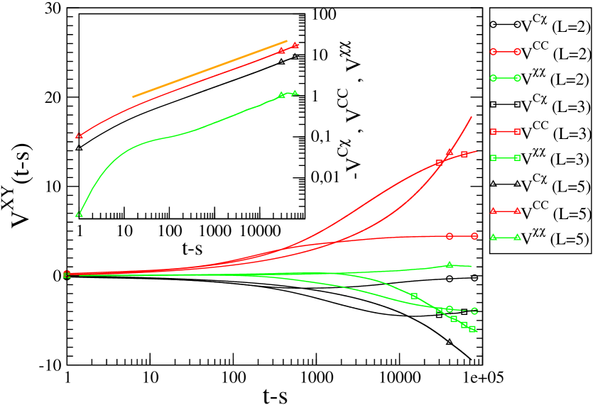
Figure 1: (Color online.) Monte Carlo simulations of the $3d$ EA model. In the main part of the figure the zero wave-vector variances $V^{XY}$ are plotted against $t-s$ in a log-linear scale, for systems of linear sizes $L=2,3,5$ in equilibrium at $T=0.8$. See the key for the color and symbol code. Averages are taken over $2.2$x$10^{8}$ realizations of the random interactions and the initial conditions. In the inset the data for $L=5$ are shown in a log-log scale (we use $-V^{C\chi}$ in order to display a positive quantity). The bold orange straight segment represents the power law $(t-s)^{\alpha}$ with $\alpha=0.4$.

The covariance $V^{C\chi}$ is negative. This can be understood since the equilibrium parametric plot $\chi(C)$ is a curve with local negative slope. Apart from the sign, this quantity behaves initially as $V^{CC}$, exhibiting a power-law growth with an exponent that is compatible with the one found for $V^{CC}$. Around $t_{M}$ the quantity $V^{C\chi}$ reaches a minimum and then grows towards an asymptotic value $V^{C\chi}_{\infty}$ which can be shown to be $V^{C\chi}_{\infty}=0$ in cases in which the system is not magnetized, $\langle\sigma_{i}\rangle=0$ CorLipSarZan10f . Indeed, in the case $L=2$, where $t_{M}$ is sufficiently short to let the system reach the asymptotic value, one has a very small final numerical value of $V^{C\chi}_{\infty}$.

Finally, $V^{\chi\chi}$ is initially positive and grows proportionally to the other two variances. Around $t_{M}$ it reaches a maximum and then decreases to a negative asymptotic value given by $V^{\chi\chi}_{\infty}=-V^{CC}_{\infty}$ CorLipSarZan10f .

In short, the initial time-difference dependence is given by

$$V^{XY}(t,s)=V^{XY}(t-s)\simeq(t-s)^{\alpha}\;\;\;\;\mbox{for}\;\;\;\;t-s\ll t_{M}(L)\;.$$ (45)

Let us stress that curves with different $L$ collapse in this power-law regime. Hence, for instance, the curves obtained for $L=5$ are also representative of a system with $L>5$ at least up to times $t\simeq 10^{5}$ MCs. This fact will be used in the next section, where a sample with $L=10$ will be studied up to $t=10^{4}$ MCs. The sum rule (24) is satisfied at all times within our numerical accuracy.

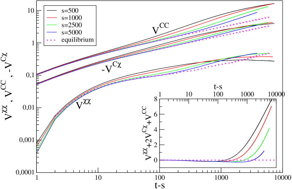
Figure 2: (Color online.) The zero wave-vector variances $V^{XY}$ after a quench of the $3d$ EA model from $T\to\infty$ to $T=0.8$. In the main panel the data are plotted against $t-s$ in a log-log scale for different values of the waiting-time $s$ given in the key. The three groups of curves are $V^{\chi\chi}$, $-V^{C\chi}$ and $V^{CC}$ from bottom to top, respectively. Averages are taken over $6.3$x$10^{7}$ realizations of the randomness and initial conditions. The (purple) dotted curves are the equilibrium behavior in the case with $L=5$. In the inset the quantity $V^{\chi\chi}+2V^{C\chi}+V^{CC}$ is plotted against $t-s$, proving that it vanishes at short time differences. Thus the equilibrium relation applies in the quasi stationary regime.

IV.1.2 Out of equilibrium behavior: variances

We now turn to the study of $V^{XY}$ in out of equilibrium conditions. We performed a quench from $T\to\infty$ to the working temperature $T=0.8$ at time $t=0$ and we followed the relaxation of a system of size $L=10$ up to $10^{4}$ MCs. We checked that in the range of times accessed in our simulations the system is free from finite size effects and remains out of equilibrium. This is probably due to the fact that, although some kind of growing length $\xi$ is present in the system others-length ; Jaubert07 ; janus , in the range of times considered here it is still of the order of a few lattice spacings (say 3 or 4 at most). The choice of the system size and range of times is dictated by the necessity to tame the colossal noise afflicting $V^{\chi\chi}$ in order to have sufficiently clean data. Indeed, increasing the system size or running for longer time enhances the noise. Concerning size, this is due to the fact that only the couples $ij$ within a distance of order $\xi$ in Eq. (44) contribute significantly to the sum, as expressed by Eq. (33), while the others introduce noisy contributions (in spite of having zero average). Regarding time, as $\xi$ increases the number $(L/\xi)^{3}$ of independent regions decreases and this also enhances the noise in the course of time. Furthermore, being two-time correlations, the $V^{XY}$ decay to zero as $t-s$ increases, making the signal/noise ratio worse. The data presented below are obtained by averaging over more than $6.3$x$10^{7}$ realizations of thermal histories, initial conditions and coupling constants.

The behavior of the variances is shown in Fig. 2. One finds $V^{CC}>0$ and $V^{C\chi}<0$, basically for the same reasons discussed in Sec. IV.1.1, while $V^{\chi\chi}$ is positive. For small time differences $t-s\lesssim\tau(s)\sim s$ one finds a quasi-equilibrium behavior: the variances depend on the time difference $t-s$ only, they superimpose on the curves found in equilibrium (for the largest size $L=5$, see the discussion at the end of Sec. IV.1.1) and the relation (24) is verified (see the inset). In short, one has

$$|V^{XY}(t,s)|\simeq(t-s)^{\alpha}\;\;\;\;\;\mbox{with}\;\;\;\;\;\alpha\simeq 0.4\;\;\;\;\;\mbox{in the stationary regime.}$$ (46)

For larger values of $t-s$ the system enters the aging regime in which non-equilibrium effects become important. One observes an explicit dependence on the two times, and a departure from the equilibrium behavior. In this regime, the $V^{XY}$ start growing faster than the power-law characteristic of the equilibrium behavior. For still larger values of $t-s$, $V^{CC}$ and $V^{C\chi}$ continue their growth steadily but in a slower logarithmic way (see Fig. 3), $\simeq(\ln t)^{b_{XY}}$. The exponents $b_{XY}$ were found to be $b_{CC}=0.86$ and $b_{C\chi}=0.52$ in the region $\ln(t/s)>1$. On the other hand, $V^{\chi\chi}$ seem to saturate to a constant value (or there could be a maximum after which it would decay, we cannot exclude this possibility). The difference of the scaling function with the ones of the other variables remains, however, only logarithmic and, in some sense, marginal. Notice that the equilibrium part of the variances is not negligible in the aging regime. Instead, increasing as a power-law, it is expected to be asymptotically dominant (although we cannot access such a long time behavior in the simulations), since $V^{XY}$ either converge to a constant value ($V^{\chi\chi}$) or grow logarithmically ($V^{CC}$ and $V^{C\chi}$).

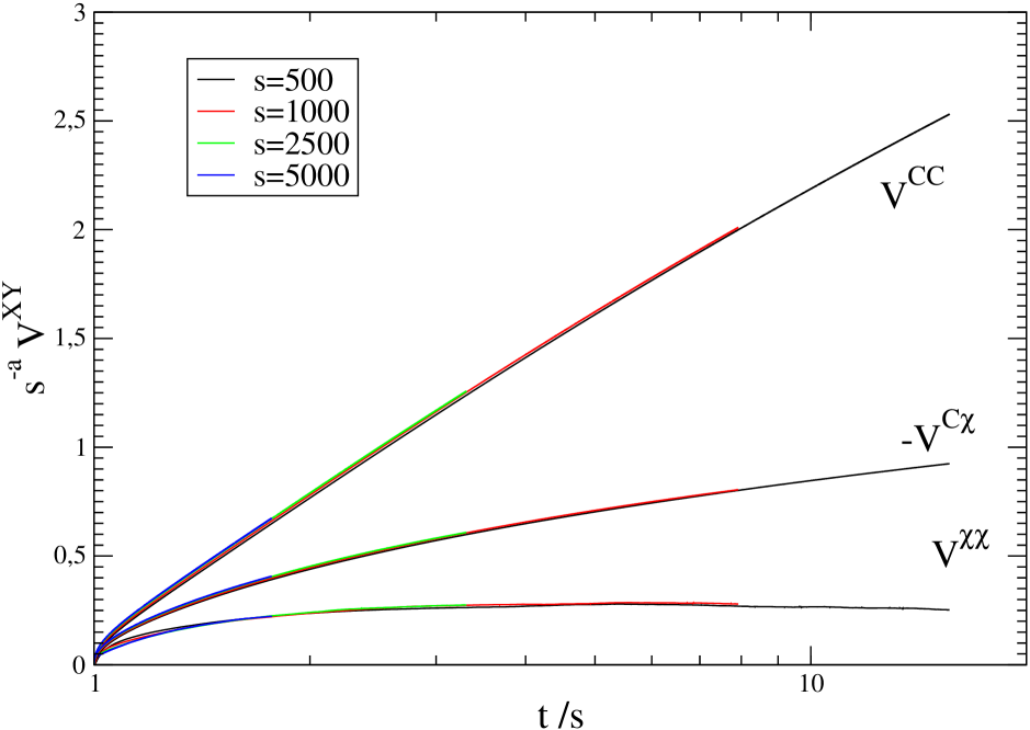
Figure 3: (Color online.) The bare data shown in Fig. 2 are collapsed by plotting $s^{-a}V^{XY}$ (with $a=0.3$) against $t/s$ in a log-linear scale for different values of $s$ (see the key). The three groups of curves are $6V^{\chi\chi}$, $-1.5V^{C\chi}$ and $V^{CC}$ from bottom to top, respectively. The factors -1.5 and 6 are used to achieve a better presentation of the data since $V^{CC}>|V^{C\chi}|\gg V^{\chi\chi}$.

Interestingly, as shown in Fig. 3, all variances obey the scaling form

$$V^{XY}(t,s)\simeq s^{a}\ f_{XY}(t/s)\;\;\;\;\;\mbox{in the aging regime,}$$ (47)

with the same exponent $a\simeq 0.3$, the same dependence on the two times $t$ and $s$ through their ratio in the remaining factor, but different scaling functions. This fact has important consequences towards the tests of the TRI scenario as we shall discuss in Sect. IV.2.

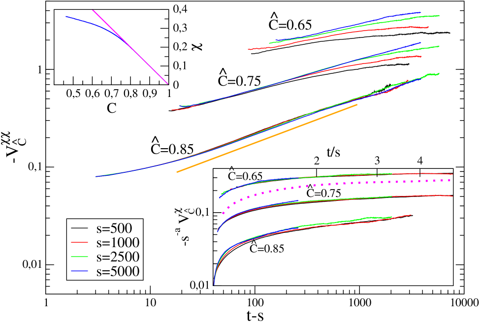
Figure 4: (Color online.) Restricted averages $-V^{\chi\chi}_{\widehat{C}}$ in the $3d$ EA model for different values of $\widehat{C}$ indicated in the figure and $s$ given in the key. The data are shown in a log-log scale. The three groups of curves have been vertically displaced for convenience. The (orange) straight segment is the power law $(t-s)^{\alpha}$, with $\alpha=0.4$. In the upper-left inset the parametric plot of $T\chi$ versus $C$ is plotted for $s=5\times 10^{3}$ MCs. The straight (magenta) line is the equilibrium behavior $T\chi=1-C$. In the lower-right inset the same curves of the main part of the figure are plotted with the rescaling of Fig. 3, namely by plotting $s^{-a}V^{\chi\chi}_{\widehat{C}}$, with $a=0.3$, against $t/s$ (in a log-log scale). The dotted (magenta) line is $s^{-a}V^{\chi\chi}$, for $s=5\times 10^{2}$ MCs.

IV.1.3 Out of equilibrium behavior: restricted averages

The restricted average of the susceptibility, $V^{\chi\chi}_{\widehat{C}}$, is shown in Fig. 4 for three values of the two-field product, $\widehat{C}=0.85$, $\widehat{C}=0.75$, and $\widehat{C}=0.65$. Interestingly enough, for all $\widehat{C}$ the sign of the restricted variance is negative, namely the opposite of the sign of the whole $V^{\chi\chi}$. From the parametric plot of $\chi$ versus $C$ (included in the upper inset) one concludes that the value $\widehat{C}=0.85$ belongs to the quasi-equilibrium regime, where $T\chi\simeq 1-C$, whereas $\widehat{C}=0.65$ is far into the aging regime. The value $\widehat{C}=0.75$ is somehow in between. For the choice $\widehat{C}=0.85$ the curves for different values of $s$ collapse, showing that $V^{\chi\chi}_{\widehat{C}}$ depend only on $t-s$ and, moreover, the data are well described by the power-law $V^{\chi\chi}_{\widehat{C}}\sim(t-s)^{\alpha}$ with an exponent that is consistent with $\alpha=0.4$ as found for the full variance $V^{\chi\chi}$ in equilibrium and in the quasi-stationary regime. Therefore for values of $\widehat{C}$ in the quasi-equilibrium regime of the parametric plot $\chi$ vs. $C$, the restricted averages have an equilibrium behavior (even for times $t-s>s$ where the whole $V^{\chi\chi}$ falls out of equilibrium). Moving towards the aging regime, for $\widehat{C}=0.75$ and $\widehat{C}=0.65$ the data collapse is progressively lost, starting from the largest values of $(t-s)/s$. Interestingly, while time translation invariance is lost, the scaling of the data transform into the non-equilibrium one, Eq. (47), found for the totally averaged variances, with the same exponent $a\simeq 0.3$. This is shown in the lower inset of Fig. 4, where we scaled the restricted averages by plotting $s^{-a}V^{\chi\chi}_{\widehat{C}}$ against $t/s$. The collapse is quite good for $\widehat{C}=0.65$ and it gets worse for increasing $\widehat{C}$. The reason why the collapse for $\widehat{C}=0.85$, although definitely worse than the one in the main panel, is not totally lost is due to the fact that the behavior $V^{\chi\chi}_{\widehat{C}}\sim(t-s)^{\alpha}$ can be written in the scaling form (47) with $\alpha$ in place of $a$. Since the exponents $a$ and $\alpha$ are not too different one would need a much larger range of $s$ in order to resolve the different curves in the lower inset of Fig. 4. Notice that for $\widehat{C}$ small enough, when the restricted averages scale as in Eq. (47) the scaling function seems to be similar to the one of the whole $V^{\chi\chi}$, apart from the change in sign. This statement is proven by comparing $-s^{-a}V^{\chi\chi}_{\widehat{C}}$ with $s^{-a}V^{\chi\chi}$ (dotted line in the inset).

IV.2 Numerical results and time-reparametrization invariance

In this Section we re-consider the numerical results of Sec. IV.1 for the spin glass and we discuss whether, how, and to which extent they may be interpreted as supporting TRI in the relaxation dynamics of the $3d$ EA model. We also report, in Sec. IV.2.2 the result of simulations of coarsening systems, where TRI is not expected to hold, to signal the differences with the dynamics of the disordered model.

IV.2.1 $3d$ Edwards-Anderson model

A first observation regards the transformation properties of the variances $V^{XY}$. We have shown in Sec. II that if TRI holds the variances must all transform in the same way, analogously to what happens for the usual two-time functions $C$ and $\chi$. According to the discussion of Sec. II.6, when scaling holds Eq. (35) must be obeyed with a unique exponent $a_{XY}$, independently of the choice of $XY$. Our findings, expressed in Eq. (47), show that scaling holds with an algebraic function $\xi(t)$, and that all the variances scale with the same exponent $a\simeq 0.3$. This result, therefore, is in agreement with the predictions of TRI. Physically, the scaling (47) with a single exponent $a_{XY}=a$ amounts to say that, fixing $t/s$, the variances of $\widehat{C}$ and $\widehat{\chi}$ are proportional. This means that basically the fluctuations of $\widehat{\chi}$ are triggered by those of $\widehat{C}$ (or vice versa). As we shall discuss in Sec. IV.2.2 the situation is very different in coarsening ferromagnets.

The behavior of the restricted variances may help us better understand this point. As expressed above, if TRI holds the non-equilibrium fluctuations of $\widehat{\chi}$ and $\widehat{C}$ are deeply related, and one can modify the former by manipulating the latter. Restricted averages are a tool to produce an extreme perturbation of the fluctuations of $\widehat{C}$, because we impose $V^{CC}_{\widehat{C}}=0$. As discussed in Sec. IV.1.2 this radically changes the behavior of the fluctuations of $\widehat{\chi}$, since even the sign of $V^{\chi\chi}_{\widehat{C}}$ is the opposite of the one of $V^{\chi\chi}$. The change in sign and the fact that $V^{\chi\chi}_{\widehat{C}}$ also scales according to Eq. (47), imply that

$${\cal V}^{\chi\chi}>\sum_{\widehat{C}}V^{\chi\chi}_{\widehat{C}}P(\widehat{C}),$$ (48)

from Eq. (26). This means that the most relevant source of fluctuations of $\widehat{\chi}$ are the fluctuations of $\widehat{C}$, while the fluctuations of $\widehat{\chi}$ which are independent of the variations of $\widehat{C}$ are less important. Again, this property is not found in coarsening systems, as we shall show in Sec. IV.2.2.

IV.2.2 Comparison with coarsening systems

TRI is not expected to hold in coarsening systems quenched below $T_{c}$ ChaCugYos06 where an infinite effective temperature Teff is developed. While the features of the $3d$ EA spin-glass discussed insofar basically agree with what one would expect in the presence of TRI, in this Section we show that the same analysis performed on a phase-ordering system, the Ising model, leads to a striking disagreement.

The behavior of the variances in the Ising model quenched below $T_{c}$ was studied numerically in CorLipSarZan10f . A scaling form analogous to Eq. (47) was found, with exponents compatible with $a_{CC}=d/2$, $a_{C\chi}=a_{\chi\chi}=1/2$ in $d=1,2$ (and conjectured to hold for higher dimensionality). The scaling functions $f_{XY}(z)$ decay as $z^{-\lambda_{XY}}$ with $\lambda_{CC}=0$, $\lambda_{C\chi}=0$, and $\lambda_{\chi\chi}=1/2$. This shows that, except at the lower critical dimension $d=1$ where the anomaly of a finite effective temperature is found LipZan00 , the variances scale with different exponents. Moreover, the behavior of the scaling functions is also very different. As discussed in Sec. II, this excludes the possibility of TRI.

The restricted averages were not studied in phase ordering kinetics so far. In order to establish how generic the behavior observed in the $3d$ EA model is, we computed these quantities in coarsening systems. We simulated the Ising model on a $d=2$ square lattice, after a quench from infinite temperature to $T=0$. The system size is $L=500$. As compared to the spin-glass, this relatively large value is needed to avoid finite size effects, since the size of correlated regions grows much faster in this problem. As a consequence, large fluctuations of $\widehat{C}$ around the average are very unlikely. Then, when computing $V^{\chi\chi}_{\widehat{C}}$ we can collect a significant statistics only in a narrower time interval than in the spin-glass case. This can be seen in Fig. 5, where the behavior of $V^{\chi\chi}$ and $V^{\chi\chi}_{\widehat{C}}$ are shown. For $V^{\chi\chi}$, we basically reproduce the results in CorLipSarZan10f (where however a quench to $T=1.5<T_{c}$ was considered). This quantity is positive and behaves as $V^{\chi\chi}\simeq s^{1/2}f_{\chi\chi}(t/s)$, where $f_{\chi\chi}(z)$ is a function which grows as $z^{1/2}$ for large $z$. Interestingly, the restricted average $V^{\chi\chi}_{\widehat{C}}$ not only has the same sign as the global average, but it superimposes almost exactly on $V^{\chi\chi}$, for $t-s$ sufficiently large (in the aging regime). This means that in the non-equilibrium regime $V^{\chi\chi}$ is completely determined by $V^{\chi\chi}_{\widehat{C}}$. According to Eq. (26), this implies

$${\cal V}^{\chi\chi}\ll\sum_{\widehat{C}}V^{\chi\chi}_{\widehat{C}}P(\widehat{C}),$$ (49)

which should be compared to the property (48) found in the $3d$ EA model. This indicates that the non-equilibrium fluctuations of $\chi$ are entirely produced at fixed $\widehat{C}$, and are then independent of those of $\widehat{C}$. This behavior, which is qualitatively different from the one observed in the $3d$ EA model, is a clear demonstration of the lack of TRI in this system.

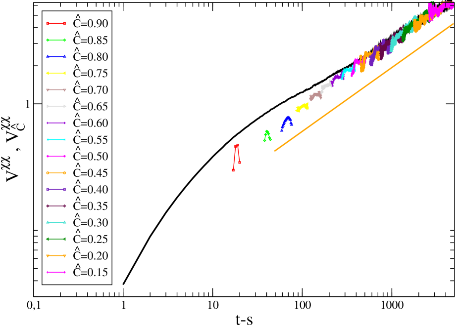
Figure 5: (Color online.) Fluctuating dynamics in the $2d$ ferromagnetic Ising model. The restricted averages $V^{\chi\chi}_{\widehat{C}}$ for different values of $\widehat{C}$ as a function of $t-s$ with fixed $s=10^{2}$ MCs are shown with (colored) line-points following the code given in the key. Similar results are found for other values of $s$. The data are shown in a log-log scale. The fully averaged variance $V^{\chi\chi}$ is displayed with a solid black line. Averages are taken over $1.1\times 10^{5}$ realizations of the randomness and initial conditions. The aging regime starts at $\widehat{C}\simeq 0.65$ where $V^{\chi\chi}_{\widehat{C}}\simeq V^{\chi\chi}$.

V Summary and conclusions

This paper is devoted to the study of the properties of fluctuations in aging systems. Specifically, we concentrate on the fluctuations of the autocorrelation and dynamic susceptibility, since the relevance of their relations to the issue of TRI was pointed out in Chamon02 ; Castillo02 ; ChaCugYos06 . In the MSRJD path-integral formulation of Langevin processes, which is overviewed in the first part of the paper, response functions are associated to the auxiliary field $i\hat{\phi}$ and hence their fluctuating parts cannot be expressed in terms of the physical field $\phi$ alone. A possible way out of this limitation is to consider moments of such fluctuating parts, since these can be related to generalized response functions which are directly measurable. In particular, in this paper we focused on the variances $V^{XY}$, because higher moments are numerically out of reach even with the highly efficient method adopted here, based on the generalization of the fluctuation-dissipation theorem out of equilibrium and beyond linear order. The behavior of these variances fits in the general framework of two-time quantities in aging systems. For short time differences a quasi-equilibrium stationary behavior is observed, while in the aging regime time-translation invariance is lost and is substituted by a different, scaling symmetry with a unique exponent $a_{XY}=a$ for all the variances. In the analytic part of the paper we derived the scaling properties of the variances and we showed that such a unique exponent is a prediction of TRI. The numerical results in the $3d$ EA therefore gives support to TRI.

In order to better characterize the fluctuations, we also computed the restricted average $V^{\chi\chi}_{\widehat{C}}$. The values of the restriction $\widehat{C}$ is an additional parameter that tunes the crossover from the quasi-equilibrium behavior to the fully aging regime. In particular, the latter is obtained letting $\widehat{C}$ be small (with respect to the EA order parameter). In this case, the restricted average scales as the fully averaged one, but its actual value is not the main contribution to the latter. These results have to be compared to the ones found in the Ising model. In this clean coarsening case the exponents $a_{XY}$ do depend on the fluctuating observables and the restricted average $V^{\chi\chi}_{\widehat{C}}$ is of the same order as the full average $V^{\chi\chi}$, showing that fluctuations of $\widehat{C}$ are not the main source for those of $\widehat{\chi}$, at variance to what it is found in the disordered model. These qualitative and quantitative differences between these two systems add to differences found in the relation between the averaged linear response and the self-correlation, i.e. the effective temperature Teff .

Our results suggest that the fluctuating out of equilibrium dynamics of the $3d$ EA model and of coarsening systems are different and that this can be related to the fact that TRI is realized in the former model while it is not in the latter. This should also be linked to the fact that the effective temperature is finite in the former and infinite in the latter cases.

These ideas should be checked numerically and analytically in other out of equilibrium systems. Natural cases to analyze are the dynamics of atomic glass models (like soft sphere, Lennard-Jones mixtures or other) with molecular dynamics or the evolution of kinetically constrained models kinetically-constrained . The Glauber Ising chain is an example that could be dealt with, possibly, analytically, exploiting the techniques derived in Mayer . Studies of critical dynamics AnnSol09 and of the relaxation of a model at its lower critical dimension should help to complete this picture.

We thank E. Lippiello, A. Sarracino, and M. Zannetti for many useful discussions. F. C. acknowledges financial support from PRIN 2007JHLPEZ (Statistical Physics of Strongly correlated systems in Equilibrium and out of Equilibrium: Exact Results and Field Theory methods) and from Université Pierre et Marie Curie and thanks the LPTHE Jussieu for hospitality during the preparation of this work. C. C. and L. F. C. thank the Universidad de Buenos Aires, Argentina, for hospitality during the last stages of this work. This work was supported in part by DOE Grant DEFG02-06ER46316 (C. C.).

References

- (1) C. Chamon, M. P. Kennett, H. E. Castillo, and L. F. Cugliandolo, Phys. Rev. Lett. 89, 217201 (2002).
- (2) H. E. Castillo, C. Chamon, L. F. Cugliandolo, and M. P. Kennett, Phys. Rev. Lett. 88, 237201 (2002). H. E. Castillo, C. Chamon, L. F. Cugliandolo, J. L. Iguain, and M. P. Kennett, Phys. Rev. B 68, 134442 (2003).
- (3) C. Chamon, P. Charbonneau, L. F. Cugliandolo, D. R. Reichman, and M. Sellitto, J. Chem. Phys. 121, 10120 (2004).
- (4) H. E. Castillo, Phys. Rev. B 78, 214430 (2008). G. A. Mavimbela and H. E. Castillo, Time reparametrization invariance in arbitrary range p-spin models: symmetric versus non-symmetric dynamics, arXiv:1011.2225.
- (5) L. D. C. Jaubert, C. Chamon, L. F. Cugliandolo, and M. Picco, J. Stat. Mech. P05001 (2007).
- (6) A. Parsaeian and H. E. Castillo, Phys. Rev. E 78, 060105(R) (2008). H. E. Castillo and A. Parsaeian, Nature Physics 3, 26 (2007). K. E. Avila, H. E. Castillo, and A. Parsaeian, Mapping dynamical heterogeneity in structural glasses to correlated fluctuations of the time variables, arXiv:1007.0520.
- (7) C. Chamon and L. F. Cugliandolo, arXiv:0704.0684, J. Stat. Mech. P07022 (2007).
- (8) L. F. Cugliandolo, Glassy dynamics, in Slow Relation and non equilibrium dynamics in condensed matter, Les Houches session 77, J-L Barrat, J. Kurchan, M. V. Feigel’man, and J. Dalibard eds. (Springer-Verlag, Berlin, 2002). G. Biroli, J. Stat. Mech. (2005) P05014.
- (9) C. Chamon, L. F. Cugliandolo, and H. Yoshino, J. Stat. Mech. P01006 (2006).
- (10) H. K. Janssen, Z. Phys. B 23, 377 (1976). H. K. Janssen in Dynamical Critical Phenomena andRelated Topics, ed. by C. P. Enz (Springer, Berlin-Heidelberg, 1979). H. K. Janssen in “From Phase Transition to Chaos”, ed. by G. Györgyi, I. Kondor, L. Sasvári, T. Tél (World Scientific, Singapore, 1992). For colored and multiplicative noise cases see C. Aron, G. Biroli, and L. F. Cugliandolo, J. Stat. Mech. P11018 (2010).
- (11) F. Corberi, E. Lippiello, A. Sarracino, and M. Zannetti, J. Stat. Mech. P04003 (2010).
- (12) E. Lippiello, F. Corberi, A. Sarracino and M. Zannetti, Phys. Rev. B 77, 212201 (2008); Phys. Rev. E 78, 041120 (2008).
- (13) E. Lippiello, F. Corberi, and M. Zannetti, Phys. Rev. E 71, 036104 (2005).
- (14) A. Andreanov, G. Biroli, J.-P. Bouchaud, A. Lefèvre, Phys. Rev. E 74, 030101 (2006). C. Aron, G. Biroli, and L. F. Cugliandolo, J. Stat. Mech. P11018 (2010).
- (15) L. F. Cugliandolo, J. Kurchan, and L. Peliti, Phys. Rev. E 55, 3898 (1997). A. Crisanti and F. Ritort, J. Phys. A 36, R181 (2003). L. F. Cugliandolo, The effective temperature, arXiv:1104.4901.
- (16) F. Corberi and L. F. Cugliandolo, J. Stat. Mech. P05010 (2009).
- (17) F. Corberi, E. Lippiello, and M. Zannetti, Phys. Rev. E 72, 056103 (2005). N. Andrenacci, F. Corberi, and E. Lippiello, Phys. Rev. E 73, 046124 (2006). E. Lippiello, F. Corberi, and M. Zannetti, Phys. Rev. E 74, 041113 (2006). F. Corberi, E. Lippiello, and M. Zannetti, Phys. Rev. E 74, 041106 (2006). R. Burioni, D. Cassi, F. Corberi, and A. Vezzani, Phys. Rev. E 75, 011113 (2007). F. Corberi, E. Lippiello, and M. Zannetti, J. Stat. Mech. P07002 (2007). F. Corberi, A. Gambassi, E. Lippiello, and M. Zannetti, J. Stat. Mech. P02013 (2008). F.Corberi, E.Lippiello, A.Mukherjee, S.Puri, and M.Zannetti, J. Stat. Mech. P030016 (2011).
- (18) F. Corberi, E. Lippiello, A. Sarracino, and M. Zannetti, Phys. Rev. E 81, 011124 (2010).
- (19) D. A. Huse, J. Appl. Phys. 64, 5776 (1988); Phys. Rev. B 43, 8673 (1991). H. Rieger, J. Phys. A 26, L615 (1993). H. Rieger, B. Steckemetz, and M. Schreckenberg, Europhys. Lett. 27, 485 (1994). J. Kisker, L. Santen, M. Schreckenberg, and H. Rieger, Phys. Rev. B 53, 6418 (1996). E. Marinari, G. Parisi, F. Ricci-Tersenghi, and J. J. Ruiz-Lorenzo, J. Phys. A 33, 2373 (2000). T. Komori, H. Takayama, and H. Yoshino J. Phys. Soc. Japan 68, 3387 (1999).
- (20) F. Belletti, A. Cruz, L. A. Fernandez, A. Gordillo-Guerrero, M. Guidetti, A. Maiorano, F. Mantovani, E. Marinari, V. Martin-Mayor, J. Monforte, A. Muñoz Sudupe, D. Navarro, G. Parisi, S. Pérez-Gaviro, J. J. Ruiz-Lorenzo, S. F. Schifano, D. Sciretti, A. Tarancon, R. Tripiccione, and D. Yllanes, J. Stat. Phys. 135, 1121 (2009).
- (21) E. Lippiello and M. Zannetti, Phys. Rev. E 61, 3369 (2000). C. Godrèche and J. M. Luck, J. Phys. A: Math. Gen. 33, 1151 (2000).
- (22) F. Ritort and P. Sollich, Adv. in Physics, 52, 219 (2003). S. Leonard, P. Mayer, P. Sollich, L. Berthier, and J. P. Garrahan, J. Stat. Mech. P07017 (2007). Kinetically Constrained Models J. P. Garrahan, P. Sollich, C. Toninelli, ”Dynamical heterogeneities in glasses, colloids, and granular media”, Eds.: L. Berthier, G. Biroli, J-P Bouchaud, L. Cipelletti and W. van Saarloos (Oxford University Press, to appear).
- (23) P. Mayer and P. Sollich J. Phys. A: Math. Gen. 37, 9 (2004).
- (24) A. Annibale and P. Sollich, J. Stat. Mech. P02064 (2009).