Quantum Information at the Interface of Light with Atomic Ensembles and Micromechanical Oscillators

Abstract

This article reviews recent research towards a universal light-matter interface. Such an interface is an important prerequisite for long distance quantum communication, entanglement assisted sensing and measurement, as well as for scalable photonic quantum computation. We review the developments in light-matter interfaces based on room temperature atomic vapors interacting with propagating pulses via the Faraday effect. This interaction has long been used as a tool for quantum nondemolition detections of atomic spins via light. It was discovered recently that this type of light-matter interaction can actually be tuned to realize more general dynamics, enabling better performance of the light-matter interface as well as rendering tasks possible, which were before thought to be impractical. This includes the realization of improved entanglement assisted and backaction evading magnetometry approaching the Quantum Cramer-Rao limit, quantum memory for squeezed states of light and the dissipative generation of entanglement. A separate, but related, experiment on entanglement assisted cold atom clock showing the Heisenberg scaling of precision is described. We also review a possible interface between collective atomic spins with nano- or micromechanical oscillators, providing a link between atomic and solid state physics approaches towards quantum information processing.

I Introduction

One of the long term goals in quantum information processing is to distribute entanglement over long distances and at large rates, in order to serve as a resource for quantum communication protocols. Such a quantum communication network will have to make use of a quantum interface which allows to efficiently perform certain primitives, such as converting light – the natural long distance carrier of quantum information – to stationary quantum memories, or creating entanglement between light and the quantum memory. Such a device will also be necessary in order to render architectures for photonic quantum computation scalable. For realizing an efficient quantum interface a strong light-matter interaction is required. Various possible approaches towards this end are being intensely explored, ranging from single atoms inside high finesse cavities specht_single-atom_2011 , via solid state devices de_riedmatten_solid-state_2008 ; hedges_efficient_2010 ; usmani_mapping_2010 ; saglamyurek_broadband_2011 , to ensembles of atoms interacting with light in free space cviklinski_reversible_2008 ; yuan_experimental_2008 ; zhao_long-lived_2009 ; zhang_creation_2009 ; zhao_millisecond_2009 ; schnorrberger_electromagnetically_2009 ; reim_towards_2010 ; radnaev_quantum_2010 ; choi_entanglement_2010 ; hosseini_high_2011 ; WFJM09 ; JWK10 ; WJKRBP10 . For comprehensive recent reviews on the various approaches based on atomic ensembles we refer to Hammerer2010 ; Sangouard2011 ; lvovsky_optical_2009 , see also miller_quantum_2010 .

Here, we focus on the most recent developments in the light-matter interface based on room temperature vapor of Cesium in glass cells WFJM09 ; JWK10 ; WJKRBP10 . The interaction between light and macroscopic Cesium ensembles at room temperature has been used extensively in many different experiments over the last decade and enabled the realization of several important quantum information processing tasks in this system including the demonstration of a quantum memory for light JSC04 , quantum teleportation between light and matter SKO06 and the generation of entanglement between two distant atomic samples using measurements and feedback operations JKP01 . The description of these and other experiments has been based on a quantum-nondemolition (QND) interaction between matter and light.
While QND interactions combined with measurements have been proven to be very successful, a new generation of developments and experiments has become possible using a more general description of the light-matter interaction. This allows not only for the accurate description of effects which have not been taken into account before and have therefore been treated as noise, but allows also for the design and implementation of protocols which go beyond the possibilities that can be realized using QND interactions, for example the purely dissipative generation of entanglement as described in Sec. III.1.

II Interaction between atomic ensembles and light

In this section, the interaction of light with an atomic ensemble is introduced and discussed for two-level systems (Sec. II.1). It is explained how it can be realized in Cesium ensembles and how this interaction can be tuned by varying externally controllable parameters (Sec. II.2). Moreover, characteristic features of the QND-Hamiltonian and a general quadratic interaction are highlighted and the respective input-output relations are discussed (Sec. II.3).

II.1 Light-matter interaction in a two-level model

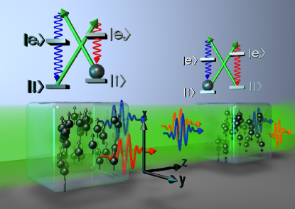
Figure 1: Light-matter interaction involving a strong $\hat{\mathbf{y}}$ polarized laser field (depicted in green) and two atomic ensembles, which are spin polarized parallel and antiparallel with respect to a homogeneous magnetic background field which is oriented along $\hat{\mathbf{x}}$ and defines the quantization axis. Atoms are assumed to posses two ground and two excited states $|\!\!\uparrow\rangle$, $|\!\!\downarrow\rangle$ and $|e_{\uparrow}\rangle$, $|e_{\downarrow}\rangle$. The strong off-resonant driving field induces diagonal transitions $|\!\!\uparrow\rangle\rightarrow|e_{\downarrow}\rangle$, $|\!\!\downarrow\rangle\rightarrow|e_{\uparrow}\rangle$ which lead to the emission of photons in $\hat{\mathbf{x}}$ polarization (corresponding to the transitions $|e_{\uparrow}\rangle\rightarrow|\!\!\uparrow\rangle$, $|e_{\downarrow}\rangle\rightarrow|\!\!\downarrow\rangle$). Due to the Zeeman splitting $\Omega$ of the atomic ground states, photons are scattered into the upper and lower sideband (shown in blue and red respectively) which are centered at $\omega_{L}\pm\Omega$, where $\omega_{L}$ is the frequency of the incident classical field.

To start with, a simple one-dimensional two-level model involving the ground states $|\!\!\uparrow\rangle$ and $|\!\!\downarrow\rangle$ is considered, as illustrated in Fig. 1, which shows a $\hat{\mathbf{y}}$-polarized laser beam propagating along $\hat{\mathbf{z}}$, and two ensembles which are strongly spin polarized and placed in a homogeneous magnetic field oriented along $\hat{\mathbf{x}}$. In this subsection, we focus on the interaction of the light field with the first ensemble which is polarized in the same direction. The light-matter interaction is assumed to be far off-resonant and therefore well within the dispersive regime. The excited levels are adiabatically eliminated under the condition $\Delta\gg\Gamma_{\mathrm{atomic}},\delta$, where $\Delta$ is the detuning, $\Gamma_{\mathrm{atomic}}$ is the largest rate at which transitions $|\!\!\uparrow\rangle\leftrightarrow|\!\!\downarrow\rangle$ occur, and $\delta$ is the Doppler width. This way, an effective interaction involving atomic ground states only is obtained. Atoms and light are described by means of the operators $a_{A}$, $a_{A}^{{\dagger}}$ and spatially localized modes $a_{L}(z)$, $a_{L}^{{\dagger}}(z)$ respectively. The creation operator $a_{L}^{{\dagger}}(z)$ FootnoteSpatiallyLocalizedModes refers to a $\hat{\mathbf{x}}$-polarized photon (the strong $\hat{\mathbf{y}}$-polarized coherent beam is treated as classical field) which is emitted in forward direction (emission of photons in other directions can be included in the form of noise terms). The operator $a_{A}^{{\dagger}}=\frac{1}{\sqrt{N_{A}}}\sum_{i=1}^{N_{A}}|\!\!\downarrow\rangle_{i}\langle\uparrow\!\!|$, where $N_{A}$ is the number of particles in the ensemble, refers to a collective atomic excitation. For strongly polarized samples, these operators can be assumed to obey bosonic commutation relations $[a_{A},a_{A}^{{\dagger}}]=1$, within the Holstein-Primakoff approximation HoP40 . The action of this collective operator on the product state $|0\rangle_{A}\equiv|\!\!\uparrow_{1},\uparrow_{2},\dots,\uparrow_{N_{A}}\rangle$, where all atoms have been initialized in $|\!\!\uparrow\rangle$, results in the symmetric coherent superposition of all $N_{A}$ possible terms representing the state where one spin in the ensemble has been flipped $a_{A}^{{\dagger}}|0\rangle_{A}=\frac{1}{\sqrt{N_{A}}}\sum_{i=1}^{N_{A}}|\!\uparrow_{1},\dots,\downarrow_{i},\dots,\uparrow_{N_{A}}\rangle$.

Atoms and light are assumed to interact according to a Hamiltonian which is quadratic in the operators describing the atomic ensemble and the light field FootnoteGaussian . The realization of strong nonlinearities in atomic systems would be desirable but represents still a formidable challenge (the realization of a cubic term would allow for universal quantum computation if arbitrary quadratic interactions are available LlB99 ).

By means of suitable local operations, any quadratic Hamiltonian describing the interaction of two one-mode continuous variable systems can be parametrized by two parameters $\gamma_{s}$ and $Z$ and expressed as a sum of a passive and an active contribution KrHGC03 ,

$$H_{\mathrm{int}}=\sqrt{2\gamma_{s}}\left(\mu H_{P}-\nu H_{A}\right),$$ (1)

where $\mu=(Z+\frac{1}{Z})/2$ and $\nu=(Z-\frac{1}{Z})/2$ (compare WFJM09 ). The passive contribution $H_{P}=a_{L}(0)a_{A}^{{\dagger}}+H.C.$ FootnotePointlike is energy conserving. If a collective atomic excitation is created, a photon is annihilated. In contrast, the active interaction $H_{A}=a_{L}(0)a_{A}+H.C.$ corresponds to the creation (or annihilation) of atomic and photonic excitations in pairs. The former interaction can be understood as the interspecies analog of a beamsplitter interaction while the latter creates entanglement and is referred to as ”squeezing interaction”. The light matter interaction considered here involves both types. The QND Hamiltonian corresponds to the special case $|\mu|=|\nu|$, where $H_{A}$ and $H_{P}$ contribute exactly with equal strength. In the simple two-level model, an imbalance $|\mu|\neq|\nu|$ can arise due to the Larmor splitting of the ground state, which leads to different detunings $\Delta+\Omega$ and $\Delta-\Omega$ for the two photon transitions associated with the active and the passive part of the interaction respectively and therefore to different effective coupling strengths and accordingly to a deviation from the QND Hamiltonian. However, in the experimental situation considered here, the detuning $\Delta$ is much larger than the Larmor splitting such that this effect is negligible (in a magnetic field of $1$ Gauss, the Zeeman shift of magnetic sublevels is about $10^{5}$Hz while the detuning is on the order of $10^{8}$ Hz). The non-QND character of the light-matter interaction in ¹³³Cs atoms is due to the fact that the levels $|\!\!\uparrow\rangle$ and $|\!\!\downarrow\rangle$ couple to several excited levels KuMSJP05 ; MKP06 ; MKMP07 ; WFJM09 as described below.

II.2 Light-matter interaction including the multi-level structure of Cesium

center

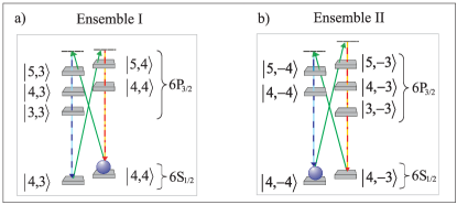
Figure 2: Off-resonant probing of the D₂ line in spin polarized ¹³³Cs ensembles as shown in Fig. 1. The strong coherent field in $\hat{y}$-polarization is depicted as full line, while the quantum fields corresponding to the blue and the red sideband are shown as dashed and dash-dotted lines respectively. Only desired transitions are shown - the level splittings are not depicted true to scale.

In contrast to the simple two-level model considered above, ¹³³Cs atoms have a multi-level structure. As illustrated in Fig. 2a, a two-level subsystem can be encoded in the $6S_{1/2}$ ground state with total spin FootnoteSpin $F=4$ by identifying the states $|\!\!\uparrow\rangle$ and $|\!\!\downarrow\rangle$ with the outermost levels corresponding to the magnetic quantum numbers (the projection of the spin along $\hat{x}$) $m_{F}=4$ and $m_{F}=3$, such that $|\!\uparrow\rangle\equiv|F=4,m_{F}=4\rangle\equiv|4,4\rangle$ and $|\!\downarrow\rangle\equiv|F=4,m_{F}=3\rangle\equiv|4,3\rangle$. In the following, we consider strongly polarized ensembles where all atoms have been initialized in state $|\!\!\uparrow\rangle$. We assume that only a small fraction of is transferred to state $|\!\!\downarrow\rangle$ during the interaction and that the population in all other levels can be neglected. The strong laser field in $\hat{\mathbf{y}}$-polarization probes the $D_{2}$ line and couples these levels off-resonantly to the excited states in $6P_{3/2}$. This way, the passive part of the interaction (corresponding to the transfer of atoms from $|\!\!\downarrow\rangle$ to $|\!\!\uparrow\rangle$ and the creation of a photon in the red sideband) involves the upper levels with $F=4,5$, while the active part of the light-matter interaction (corresponding to the transfer $|\!\uparrow\rangle\rightarrow|\!\downarrow\rangle$ and the creation of a photon in the blue sideband) involves the manifolds with $F=3,4,5$. The corresponding $Z$-parameter can be easily determined if the detuning and the corresponding Clebsch-Gordan coefficients are known. In this specific case, one obtains $Z=\left(\mu+\nu\right)=2.5$ for blue detuning $\Delta=850$MHz with respect to the state with total spin $F=5$ within $6P_{3/2}$.

In general, $Z$ can be calculated as follows. The effective rate for ground state transitions $|\!\!\uparrow\rangle\leftrightarrow|\!\!\downarrow\rangle$ involving the excited state $|l\rangle$ is given by $\Gamma_{|a\rangle\rightarrow|l\rangle\rightarrow|b\rangle}=\Omega_{\text{R}}^{2}|\frac{c_{al}c_{lb}}{\Delta_{l}+i\gamma_{l}}|^{2}\gamma_{l}\approx\Omega^{2}_{\text{R}}\frac{|c_{al}c_{lb}|^{2}}{\Delta_{l}^{2}}\gamma_{l}$, where $\Omega_{\text{R}}^{2}$ is the Rabi frequency of the applied laser field FootnoteAppliedField , $c_{al}$ and $c_{lb}$ are the Clebsch-Gordan coefficients for the transitions $|a\rangle\rightarrow|l\rangle$ and $|l\rangle\rightarrow|b\rangle$, $\gamma_{l}$ is the natural line width of the excited state and $\Delta_{l}\gg\gamma_{l}$ was assumed. If several excited states contribute, the different paths can interfere and the effective rate for the off-resonant transition $|a\rangle\rightarrow|b\rangle$ is therefore given by the sum $\Gamma_{|a\rangle\rightarrow|b\rangle}=\Omega^{2}_{\text{R}}|\sum_{l}\frac{c_{al}c_{lb}}{\Delta_{l}}|^{2}\gamma$, where the line widths of the involved excited levels have been assumed to be approximately equal. If the the ratio $r^{2}=\frac{\Gamma_{|\downarrow\rangle\rightarrow|\uparrow\rangle}}{\Gamma_{|\uparrow\rangle\rightarrow|\downarrow\rangle}}=\frac{\mu^{2}}{\nu^{2}}$ is calculated, $Z^{2}=\frac{r+1}{r-1}$ can be determined.

If the sign of the detuning is changed (using for example red instead of blue detuning) the character of the interaction can be changed from the predominantly passive to the active type. This can also be achieved by interchanging the polarization of the classical and the quantum field. As illustrated in Fig. 2a, using a $\hat{\mathbf{x}}$-polarized classical field (driving vertical transitions, in this picture) and correspondingly a quantum field in $\hat{\mathbf{y}}$-polarization (associated with diagonal transitions FootnoteSpin ) would involve the excited levels with $F=3,4,5$ for the passive part of the interaction and the levels with $F=4,5$ for the active one (as opposed to the setting discussed above, where it is the other way round). The imbalance between the active and the passive part becomes less pronounced for large detunings. If $\Delta$ is much larger than the hyperfine splitting of the excited states, the interaction Hamiltonian can be well approximated by $H^{\mathrm{QND}}$ WFJM09 ; Hammerer2010 .

II.3 Input-output relations and characteristic properties of the interaction

In the following, the canonical quadratures $x=(a+a^{{\dagger}})/\sqrt{2}$ and $p=-i(a-a^{{\dagger}})/\sqrt{2}$ will be used. The atomic quadratures $x_{A}$ and $p_{A}$ can be identified with the transverse components of the collective spin. Since we consider strongly polarized atomic ensembles (see Sec. II.2), the macroscopic spin in $\hat{\textbf{x}}$-direction can be described by a ${I}\!\!\!\!C$-number. The deviation from perfect $\hat{\mathbf{x}}$-alignment is described by the collective spins in $\hat{\mathbf{y}}$ and $\hat{\mathbf{z}}$ direction $J_{y}=\sum_{i=1}^{N}\sigma_{i}^{y}$ and $J_{z}=\sum_{i=1}^{N}\sigma^{i}_{z}$, where the operators $\sigma^{i}_{y}$ and $\sigma^{i}_{z}$ denote the $y$ and $z$ component of the i^th atom respectively such that within the Holstein-Primakoff approximation $x_{A}=J_{y}/\sqrt{|\langle J_{x}\rangle|}$ and $p_{A}=J_{z}/\sqrt{|\langle J_{x}\rangle|}$. In terms of quadratures, the quadratic Hamiltonian introduced above (1) is given by

$$H_{\mathrm{int}}=\sqrt{2\gamma_{s}}(Zp_{A}p_{L}(0)+\frac{1}{Z}x_{A}x_{L}(0)).$$ (2)

As will become apparent in Sec. II.3.2 (see Eq. (4)), $Z$ FootnoteSqueezing quantifies the squeezing (and corresponding anti-squeezing) of the variances involved in the process WFJM09 , while $\gamma_{s}$ FootnoteSwapping characterizes the rate at which atomic and light quadratures are swapped. In the balanced case ($\mu=\nu$), $H_{\mathrm{int}}$ reduces to the QND Hamiltoninan $H_{QND}\propto p_{A}p_{L}(0)$. Below, we introduce the input-output relations describing the light-matter interaction and highlight characteristic features of the imbalanced and the balanced (QND) type.

II.3.1 QND interaction

The balanced type of the interaction corresponding to the limit $Z\rightarrow\infty$ (with $\sqrt{2\gamma_{s}}\cdot Z=\kappa$, where $\kappa$ is constant), $H_{QND}=\kappa p_{A}p_{L}$ is referred to as quantum-nondemolotion interaction since the $p$-quadratures of atoms and light are conserved. The input-output relations for a single cell in the absence of a magnetic field HaPC05 are given by

$$x_{A}^{out} = x_{A}^{in}+\kappa p_{L}^{in},\ \ \ \ \ \ p_{A}^{out}=p_{A}^{in},$$

$$x_{L}^{out} = x_{L}^{in}+\kappa p_{A}^{in},\ \ \ \ \ \ p_{L}^{out}=p_{L}^{in},$$ (3)

where $x_{L}^{in}=\frac{1}{\sqrt{T}}\int_{0}^{T}dt\bar{x}_{L}(ct,0)$ and $x_{L}^{out}=\frac{1}{\sqrt{T}}\int_{0}^{T}dt\bar{x}_{L}(ct,T)$ (analogous definitions hold for $p_{L}^{in}$ and $p_{L}^{out}$). Here, the variable transformation $x_{L}(r,t)\rightarrow x_{L}(ct-\xi,t)=\bar{x}_{L}(\xi,t)$ has been made. The spatial variable $\xi=ct-z$ refers to a coordinate system which is fixed to the propagating light pulse. $\xi=0$ refers to the front part of the pulse which enters the ensemble first, while the rear part which passes last corresponds to $\xi=cT$.

Shot-noise limited measurements of the collective spin by homodyne detection of the light field require the application of magnetic fields. In the presence of magnetic fields, atomic ground states are Zeeman-shifted by the Larmorsplitting $\Omega$ as shown in Fig. 2 (here and in the following, we use $\hbar=1$).

The scattering of a narrow-band classical field with central frequency $\omega_{c}$ leads therefore to the emission of photons into sideband modes, which are centered around $\omega_{c}\pm\Omega$ in frequency space, as illustrated in Fig. 1 which allows for noise reduced measurements on the light field using lock-in methods (see Ju03 ). In the time domain, atomic information is mapped to $\sin(\Omega t)$ and $\cos(\Omega t)$ modulated light modes

$$x_{f,cos}^{in} = \sqrt{\frac{2}{T}}\int_{0}^{T}dtf(t)\cos(\Omega t)\bar{x}_{L}(ct,0),$$

$$x_{f,cos}^{out} = \sqrt{\frac{2}{T}}\int_{0}^{T}dtf(t)\cos(\Omega t)\bar{x}_{L}(ct,T).$$

$x_{f,cos/sin}$ and $p_{f,cos/sin}$ refer to a light mode with an arbitrary envelope function $f(t)$, which varies slowly on the time scale set by the Larmor frequency $\Omega$. The envelope function $f(t)$ is normalized such that $\frac{1}{T}\int_{0}^{T}dtf(t)^{2}=1$. In the limit $\Omega T\gg 1$, which is well fulfilled under the experimental conditions considered here, sine and cosine modulated modes are canonical and independent $[x_{f,sin/cos},p_{f,sin/cos}]=i$, $[x_{f,sin/cos},p_{f,cos/sin}]=0$. The input-output relations for a single ensemble in a magnetic field involve an infinite hierarchy of coupled backaction modes HaPC05 , whose envelope functions are given by Legendre polynomials (the general expressions can be found in HPC06 ). If a setup as shown in Fig. 1 with antiparallel oriented spins, or equivalently, antiparallel oriented magnetic fields, is considered, the input-output relations simplify considerably since all photonic contributions except for the lowest order cancel such that

$$x_{A,cos}^{out} = x_{A,cos}^{in}+\kappa p_{L_{0},cos}^{in},$$ (4)

$$p_{A,cos}^{out} = p_{A,cos}^{in},$$

$$x_{L_{0},cos}^{out} = x_{L_{0},cos}^{in}+\kappa p_{A,cos}^{in},$$

$$p_{L_{0},cos}^{out} = p_{L_{0},cos}^{in},$$

$$x_{A,sin}^{out} = x_{A,sin}^{in}+\kappa p_{L_{0},sin}^{in},$$

$$p_{A,sin}^{out} = p_{A,sin}^{in},$$

$$x_{L_{0},sin}^{out} = x_{L_{0},sin}^{in}+\kappa p_{A,sin}^{in},$$

$$p_{L_{0},sin}^{out} = p_{L_{0},sin}^{in},$$

where the EPR-operators $x_{A,cos}=(x_{A,I}+x_{A,II})/\sqrt{2}$, $p_{A,cos}=(p_{A,I}+p_{A,II})/\sqrt{2}$ and $x_{A,sin}=-(p_{A,I}-p_{A,II})/\sqrt{2}$, $p_{A,sin}=(x_{A,I}-x_{A,II})/\sqrt{2}$ have been used. A comparison of Eq. (II.3.1) with Eq. (4) shows that the the input output relations for two atomic ensembles which are Larmor-precessing in opposite directions are formally equivalent to two independent sets of input-output relations describing the simple case of a single ensemble in the absence of a magnetic field.

This antiparallel setup has for instance been used for the implementation of a quantum memory for light JSC04 and entanglement generation between two ensembles JKP01 . Since only the $p$-quadrature of each set of variables is mapped by the interaction, the realization of a quantum memory required the measurement of the $p$-quadrature of the light field and a subsequent feedback operation on the atoms in order to transfer both quadratures $x_{L_{0},sin/cos}$ and $p_{L_{0},sin/cos}$. Also the creation of entanglement based on a QND interaction requires measurements on the light field. The light-matter interaction itself does not create entanglement, but it allows for a projection onto an Einstein-Podolski-Rosen (EPR) entangled state with squeezed non-local variances $\mathrm{var}\!\left(x_{A,sin}\right)$ and $\mathrm{var}\!\left(x_{A,cos}\right)$ if $x_{L_{0},sin}$ and $x_{L_{0},cos}$ are measured.

However, an ideal beamsplitter or squeezing interaction which would allow for perfect mapping or for the creation of infinitely entangled states in the limit $\kappa\rightarrow\infty$, can be realized based on a QND interaction by means of a double-pass scheme FiSOP05 ; QuantumMemory ; SM06 , in which one of the two contributions, $H_{P}$ or $H_{A}$ is cancelled by interference.

II.3.2 Non-QND interaction

In the following, we consider the general interaction described by Eq. (2). The input-output relations for a single cell in a magnetic field are given by

$$\left(\begin{array}[]{c}x_{A}^{out}\\ p_{A}^{out}\\ \end{array}\right) = e^{-\gamma_{s}T}\left(\begin{array}[]{c}x_{A}^{in}\\ p_{A}^{in}\\ \end{array}\right)+\sqrt{1-e^{-2\gamma_{s}T}}\left(\begin{array}[]{c}x_{+,\mathrm{r}}^{in}\\ p_{+,\mathrm{r}}^{in}\\ \end{array}\right),$$

$$\left(\begin{array}[]{c}x_{-,\mathrm{r}}^{out}\\ p_{-,\mathrm{r}}^{out}\\ \end{array}\right) = e^{-\gamma_{s}T}\left(\begin{array}[]{c}x_{+,\mathrm{r}}^{in}\\ p_{+,\mathrm{r}}^{in}\\ \end{array}\right)-\sqrt{1-e^{-\gamma_{s}T}}\left(\begin{array}[]{c}x_{A}^{in}\\ p_{A}^{in}\\ \end{array}\right),$$

where the exponentially rising/falling reading modes with quadratures $x_{\pm,\mathrm{r}}$, $p_{\pm,\mathrm{r}}$ are given by

$$\left(\begin{array}[]{c}\!\!x_{\pm,\mathrm{r}}^{in}\!\!\\ \!\!p_{\pm,\mathrm{r}}^{in}\!\!\\ \end{array}\right)\!\! = \!\!\frac{1}{2}\left(\!\left(Z\!+\!\frac{1}{Z}\right)\left(\begin{array}[]{c}\!\!x_{\pm,us}^{in}\!\!\\ \!\!p_{\pm,us}^{in}\!\!\\ \end{array}\right)\!+\!\left(Z\!-\!\frac{1}{Z}\right)\left(\begin{array}[]{c}\!\!p_{\pm,ls}^{in}\!\!\\ \!\!x_{\pm,ls}^{in}\!\!\\ \end{array}\right)\!\right).$$

$x_{\pm,us}$, $p_{\pm,us}$ and $x_{\pm,ls}$, $p_{\pm,ls}$ refer to exponentially modulated modes

$$\left(\begin{array}[]{c}x_{\pm,us}^{in}\\ p_{\pm,us}^{in}\\ \end{array}\right) = \frac{\sqrt{2\gamma_{s}}}{N_{\pm}}\int_{0}^{T}d\tau e^{\pm\gamma_{s}\tau}R(\tau)\left(\begin{array}[]{c}\bar{p}_{L}(c\tau,0)\\ -\bar{x}_{L}(c\tau,0)\\ \end{array}\right),$$

$$\left(\begin{array}[]{c}p_{\pm,ls}^{in}\\ x_{\pm,ls}^{in}\\ \end{array}\right) = \frac{\sqrt{2\gamma_{s}}}{N_{\pm}}\int_{0}^{T}d\tau e^{\pm\gamma_{s}\tau}R(\tau)\left(\begin{array}[]{c}\bar{p}_{L}(c\tau,0)\\ \bar{x}_{L}(c\tau,0)\\ \end{array}\right),$$

which are located at $\omega_{c}\pm\Omega$ in frequency space respectively (compare Fig. 1). The subscripts $us$ and $ls$ refer accordingly to the upper and lower sideband. The normalization constants $N_{+}$, $N_{-}$ and the rotation matrix $R(\tau)$ are given by

$$N_{+} = \sqrt{e^{\frac{\kappa^{2}}{Z^{2}}}-1},\ \ N_{-}=\sqrt{1-e^{-\frac{\kappa^{2}}{Z^{2}}}},$$

$$R(\tau) = \left(\begin{array}[]{cc}\cos(\Omega\tau)&-\sin(\Omega\tau)\\ \sin(\Omega\tau)&\cos(\Omega\tau)\\ \end{array}\right).$$

As outlined above, the setup involving two antiparallel oriented ensembles in magnetic fields can be conveniently described in terms of EPR modes such that two independent sets of equations are obtained

$$\left(\begin{array}[]{c}\!\!x_{\text{\tiny{A,sin\!\!/\!cos}}}^{out}\!\!\\ \!\!p_{\text{\tiny{A,sin\!\!/\!cos}}}^{out}\!\!\\ \end{array}\right)\!\!\!\! = \!\!\!e^{-\gamma_{s}T}\!\!\left(\begin{array}[]{c}\!\!x_{\text{\tiny{A,sin\!\!/\!cos}}}^{in}\!\!\\ \!\!p_{\text{\tiny{A,sin\!\!/\!cos}}}^{in}\!\!\\ \end{array}\right)\!\!+\!\!\sqrt{\!1\!\!-\!\!e^{-2\gamma_{s}T}}\!M_{Z}\!\!\left(\begin{array}[]{c}\!\!p_{\text{\tiny{+,sin\!\!/\!cos}}}^{out}\!\!\\ \!\!x_{\text{\tiny{+,sin\!\!/\!cos}}}^{out}\!\!\\ \end{array}\!\right),$$ (17)

$$\left(\begin{array}[]{c}\!\!x_{\text{\tiny{-,sin\!\!/\!cos}}}^{out}\!\!\\ \!\!p_{\text{\tiny{-,sin\!\!/\!cos}}}^{out}\!\!\\ \end{array}\right)\!\!\!\! = \!\!\!e^{-\gamma_{s}T}\!\!\left(\begin{array}[]{c}\!\!x_{\text{\tiny{+,sin\!\!/\!cos}}}^{in}\!\!\\ \!\!p_{\text{\tiny{+,sin\!\!/\!cos}}}^{in}\!\!\\ \end{array}\right)\!\!+\!\!\sqrt{\!1\!\!-\!\!e^{-2\gamma_{s}T}}\!M_{Z}\!\!\left(\begin{array}[]{c}\!\!p_{\text{\tiny{A,sin\!\!/\!cos}}}^{out}\!\!\\ \!\!x_{\text{\tiny{A,sin\!\!/\!cos}}}^{out}\!\!\\ \end{array}\!\right)$$ (24)

where the matrix $M_{Z}$ is given by

$$M_{Z}=\left(\begin{array}[]{cc}\!Z\!&\!0\!\\ \!0\!&\!-\!\frac{1}{Z}\!\\ \end{array}\right).$$

Due to the inherent backaction of the interaction, these input-output relations display an exponential scaling in the coupling strength, as opposed to Eq. (4). This is due to the fact that the light field is continuously mapped to both atomic quadratures $x_{A}$ and $p_{A}$ which in turn are mapped to the passing photonic field. This way, the light field passing the ensembles at time $t=t_{1}$ is subject to an interaction which involves the photonic contributions which have been mapped to the atomic state during the time $t<t_{1}$ and experiences therefore an effective backaction mediated by the atoms.

An imbalanced quadratic interaction ($|\mu|\neq|\nu|$) allows for the realization of protocols which are not possible employing an interaction of QND-type, for example the creation of entanglement by dissipation which has been recently demonstrated using atomic ensembles at room temperature EbDExperiment ; EbDtheory (see Sec. III.1). More specifically, the atomic system interacts with the continuum of electromagnetic modes $a_{\mathbf{k}}$. In the ideal case, the interaction between the two ensembles constituting the system and the continuum of light modes, which acts as environment, is engineered such that the atomic system is driven into an entangled steady state. In contrast to standard approaches DLCZ01 ; K08 ; Hammerer2010 this method creates unconditional entanglement, since no measurements on the light field (bath) are required FootnoteBath . This feature is due to the fact that the light field possesses an infinite number of degrees of freedom, such that a non-unitary dynamics which drives the system towards a fixed state can be implemented. Due to this property, the corresponding interaction is referred to as dissipative process. Since dissipative processes are most naturally described in terms of master equations, we will use this formalism in the remainder of this section rather than input-output relations. Both descriptions are equivalent. The master equation for the atomic system discussed below can for example be obtained by considering the interaction of atoms and light as discussed above for small time steps $\delta t$ and tracing out the light field. The Hamiltonian governing the light-matter interaction for two ensembles in a magnetic field as shown in Fig. 1 can be written in the form Footnote6

$$H\propto\int_{\Delta\omega_{\text{ls}}}d\mathbf{k}\left(Aa_{\mathbf{k}}^{{\dagger}}+A^{{\dagger}}a_{\mathbf{k}}\right)+\int_{\Delta\omega_{\text{us}}}d\mathbf{k}\left(Ba_{\mathbf{k}}^{{\dagger}}+B^{{\dagger}}a_{\mathbf{k}}\right),$$

where $a_{\mathbf{k}}$ is the creation operator for a photon with wave vector $\mathbf{k}$ and the integrals cover narrow bandwidths $\Delta\omega_{\text{ls}}$ and $\Delta\omega_{\text{us}}$ centered around the lower and upper sideband respectively. The atomic operators $A$ and $B$ FootnoteOperatorsDefinition are given by

$$A = \mu J^{-}_{\text{I}}-\nu J^{-}_{\text{II}},$$ (26)

$$B = \mu J^{+}_{\text{II}}-\nu J^{+}_{\text{I}},$$

where $J^{+}=J_{y}-iJ_{z}$ and $J^{-}=J_{y}+iJ_{z}$. We assume Markov dynamics, which is well justified for optical frequencies such that a master equation of Lindblad form is obtained after tracing out the photonic modes

$$\frac{d}{dt}\rho = d\ \frac{\Gamma}{2}\left(A\rho A^{{\dagger}}-A^{{\dagger}}A\rho+B\rho B^{{\dagger}}-B^{{\dagger}}B\rho+H.C.\right)$$

$$+ {\cal L}_{\rm noise}\rho,$$

where $\rho$ is the reduced atomic density operator, $d$ is the resonant optical depth of one ensemble and $\Gamma$ is the effective single particle decay rate. The first term on the right describes the ideal case, while the second one accounts for noise processes. The master equation can also be derived starting from the input-output relations (17) introduced above by identifying $\gamma_{s}=d\Gamma$ Footnote7 . In the ideal case (${\cal L}_{\rm noise}\rho=0$), the steady state of the dissipative evolution is given by $\rho_{\mathrm{EPR}}=|\Psi_{\mathrm{EPR}}\rangle\langle\Psi_{\mathrm{EPR}}|$ with

$$A|\Psi_{\mathrm{EPR}}\rangle=B|\Psi_{\mathrm{EPR}}\rangle=0.$$

Since the jump operators $A$ and $B$ are nonlocal (see Eq. (26)), the steady state $|\Psi_{\mathrm{EPR}}\rangle$ corresponds to an EPR-entangled state where the collective spins in $\hat{y}$ and $\hat{z}$ direction are strongly correlated, such that $\mathrm{var}(J_{yI}-J_{yII})+\mathrm{var}(J_{zI}-J_{zII})<|\langle J_{xI}\rangle|+|\langle J_{xII}\rangle|$ Footnote8 .

It can be shown that this steady state is unique for $|\mu|\neq|\nu|$ EbDtheory (in the QND case no unique steady state exists). This way, the desired state is reached independently of the initial state. The initialization of the system in a well defined fiducial state, which is typically considered a critical issue DiVincenzo2000 , is therefore rendered unnecessary. Moreover, the resulting state is stabilized by the dissipative dynamics and can be maintained, in principle, for arbitrary long times. Using these ideas, it is therefore possible to overcome important restrictions set by the limited coherence times of quantum systems.

III Experiments based on Faraday Interaction beyond QND

In this section a series of experiments based on the described theory are presented. In all realizations considered here, two ensembles of Cesium atoms at room temperature are coupled to light in a controlled fashion. This setup proves to be a versatile tool to realize many different experiments on the quantum level WFJM09 , including quantum communication protocols JWK10 as well as metrology on the quantum sensitivity level WJKRBP10 .

The basic setup is sketched in Fig. 3. The two ensembles are prepared in oppositely oriented coherent spin states (CSS). This is achieved by optically pumping the atoms of the ensembles in $m_{F}=\pm 4$ in the $\hat{\mathbf{x}}$-direction respectively. The atoms are situated in a magnetic field $B$ which leads to a splitting of the magnetic sublevels by $\Omega$. The circularly polarized pump lasers are depicted in green and the inset of Fig. 3 shows the atomic level structure, indicating laser frequencies and polarization. The strong probe beam which is initially polarized in $\hat{\mathbf{y}}$-direction transverses the atoms in the $\hat{\mathbf{z}}$-direction. Behind the cells the detection system is set up. The light observable of interest is the Stokes operator $S_{2}\propto x_{L}$ which can be measured with polarization homodyning techniques. The signal from the detectors is analyzed at the Larmor frequency $\Omega$ since we are interested in the spins in the rotating frame. Additionally the measurement outcome can be weighted with suitable mode-functions $f(t)$ to achieve an optimal signal. In the following three different experiments realized in the setup are described.

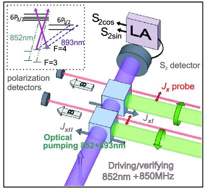
Figure 3: Experimental setup. The inset shows the atomic level scheme in $\hat{\mathbf{x}}$-quantization. The relevant laser frequencies and polarizations are indicated. The dc polarization detectors measure the Faraday rotation angle $\Theta$ proportional to the macroscopic spin $J_{x}$. The $S_{2}$ detector signal processed by the lock-in amplifier (LA). The evaluated modes $x_{f,\text{cos}}\propto\int_{0}^{T}\cos(\Omega t)f(t)S_{2}(t)dt$ and $x_{f,\text{sin}}\propto\int_{0}^{T}\sin(\Omega t)f(t)S_{2}(t)dt$ with the interaction duration $T$ are used to determine the atomic quantum spin components $J_{y,z}$ in the rotating frame. The used mode functions $f(t)$ are mostly exponentially decaying or growing functions. The inset shows the optical pumping scheme.

III.1 Entanglement generated by dissipation and steady state entanglement of two macroscopic objects

The input-output-relations (17) arising from the non-QND model for the scenario sketched in Fig. 3 reveal interesting possibilities, when evaluated for long interaction times:

$$x_{-,\text{cos/sin}}^{\text{out}}\!\! \rightarrow \!\!Zp_{A,\text{cos/sin}}^{\text{in}},\hskip 8.5359ptp_{-,\text{cos/sin}}^{\text{out}}\!\!\rightarrow\!\!-\frac{1}{Z}x_{A,\text{cos/sin}}^{\text{in}}$$

$$x_{A,\text{cos/sin}}^{\text{out}}\!\! \rightarrow \!\!Zp_{+,\text{cos/sin}}^{\text{in}},\hskip 8.5359ptp_{A,\text{cos/sin}}\!\!\rightarrow\!\!-\frac{1}{Z}x_{+,\text{cos/sin}}^{\text{in}}.$$ (27)

The two systems, light and atoms, swap state and individually get squeezed by the factor $Z^{2}$ if both systems start in a minimum uncertainty state. In WFJM09 the observation of two mode squeezing of light in $p_{-,\text{cos}}^{\text{out}}$ and $p_{-,\text{sin}}^{\text{out}}$ is reported. There a noise reduction of 3dB was achieved. At the same time the equations predict a reduction in the noise of the atomic operators $p_{A,\text{cos}}$ and $p_{A,\text{sin}}$, indicating a possibility to achieve entanglement between the two ensembles via this light-atom interaction. Atomic entanglement is of special interest as it can in principle be distributed and then stored until one wishes to use it. However, exactly the storage represents a major problem in most previously conducted atomic entanglement experiments. Atomic entangled states proved to be extremely fragile, whether they were generated by mapping of squeezed light onto atoms Honda2008 ; Appel2008 , by measurement JKP01 ; ChRFPEK05 ; EiAMFZL05 ; MCJ06 ; YCZC08 ; AWO09 , atomic interactions GZN10 ; RB10 or a nonlinear interaction mediated by light FKJ08 . The coupling to the environment leads to decoherence which until now irresistibly was followed by the disappearance of entanglement after a certain time. Several proposals have been made, as to how to use carefully engineered environments to create a situation where entanglement is reached by dissipation to overcome this shortcoming PH02 ; KC04 ; DMK08 ; VWC09 ; BMS11 . More specifically, dissipatively generated entanglement was proposed for our system in EbDtheory . This theoretical approach is an extension of the presented theory, in which spontaneous emission in the continuum of modes and atomic decay mechanisms are considered. The understanding gained this way is that entanglement between the two ensembles is generated by the interference of different processes in the two ensembles for which an indistinguishable photon is emitted into the common mode. The processes in the forward direction are collectively enhanced and a photon emitted into for example the upper sideband stands for an atomic excitation in ensemble one, or an annihilation in ensemble two.

The pulse sequence for an entanglement generation experiment is shown on top in Fig. 4a. However, when the experiment was carried through, the proposed unconditional entanglement generation procedure lead only to a long entanglement duration of around 15ms, but not the wanted steady state entanglement. The reason is the loss of atoms from the atomic two level system of relevance due to decay. To counteract this depopulation, two pump lasers are added. First a pump laser on resonance with the $F=4\rightarrow F^{\prime}=4$ transition on the $D_{1}$ line is added (depicted by the blue lines in the inset of Fig. 3), for which $m=4$ is a dark state. This incoherent process leads to an increase in the duration of unconditional entanglement to $\sim 40ms$. In this scenario atoms still undergo transitions to the $F=3$ ground state, effectively reducing the number of atoms participating in the interaction. To avoid this depletion, a repump beam is added (green lines in the inset of Fig. 3). In this experimental setting (bottom of Fig. 4a), a steady state is achieved after few ms, but no entanglement can be deduced from the noise of the collective atomic operators. However, when a measurement on the light output is added to the protocol JKP01 , a steady state which is entangled conditioned on the continuous measurement outcomes of $x_{L}$ arises. The principle of this procedure is sketched in Fig. 4b. In Krauter2011 such a long time entanglement was measured for up to an hour, where a 1dB noise reduction was achieved.

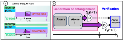
Figure 4: (a) Pulse sequence. In the upper sequence a CSS is prepared by optical pumping after which the atomic state evolves in the presence of the probe light. Below a pulse sequence for the experimental realization of a steady state scenario with high atomic population of the relevant atomic sublevels is shown. Here, the pump lasers are not completely turned off but ramped down to optimized strength.(b) Schematic illustration of entanglement generation in the steady state and verification. The signal taken at $t<T$ is given to the verifier as additional information to reduce the noise of the collective atomic operators. The signal from the detector D for times $t>T$ is used for verification of entanglement. This corresponds to the pulse sequence presented at the bottom of (a).

III.2 Quantum memory for entangled two-mode squeezed states

A quantum memory for light is a key element for the realization of future quantum information networks. The basic principle of such a memory protocol is the transfer of the quantum state of light to a storage medium. Here, this means the canonical quantum variables of light are transferred to the corresponding atomic ones. We know from the input-output equations presented in section II.3, that if we could achieve the long interaction time regime, the underlying interaction would swap the states of the two systems (see Eq. (27)). However, as this is not possible for our experimental realization due to decoherence, a trick is applied to achieve the desired state transfer; the $x_{L_{0},\text{cos/sin}}$ of the outgoing light are measured and the measured results are fed back to the atoms via RF magnetic fields: $p_{A,\text{cos/sin}}^{\text{out}}-g\cdot x_{+,\text{cos/sin}}^{\text{out}}$. Following eq. (17) and assuming a coupling constant $\kappa=\sqrt{1-e^{-2\gamma_{s}T}}\cdot Z=1$ and a feedback gain $g$ which is also $1$, the collective atomic operators are then left as:

$$P_{A,\text{cos/sin}}^{\text{fin}} = -x_{+,\text{cos/sin}}^{\text{in}},$$ (28)

$$x_{A,\text{cos/sin}}^{\text{fin}} = \sqrt{1-\frac{1}{Z^{2}}}x_{A,\text{cos/sin}}^{\text{in}}+p_{+,\text{cos/sin}}^{\text{in}}$$

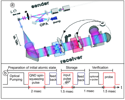
Figure 5: Two-mode entangled (squeezed) light is generated by an optical parametric amplifier (OPA). A variable displacement of the state is achieved by injecting a coherent input into the OPA which is displaced with help of electro-optical modulators (EOM). The output of the OPA is shaped by a chopper, and combined on a polarizing beamsplitter with the local oscillator (LO) beam, such that the squeezed light is only on during the second probe pulse. A beam shaper and a telescope create an expanded flat-top intensity profile. The light is then send to the memory consisting of two oppositely oriented ensembles and the homodyne detection system. The detector signal is processed electronically and used as feedback onto the spins via RF magnetic field pulses. Below, the pulse sequence is shown. After preparing the squeezed spins state, the actual storage takes place, followed by a verification pulse.

Clearly the input light state is mapped onto the atoms with some additional noise coming from the atomic $x$ operators. Compared to a protocol based on a QND interaction and feedback, this additional noise is suppressed. A memory based on a similar protocol was conducted for coherent states in the setup exceeding the achievable fidelity for any classical memory JSC04 . The next obvious step was to map non classical states, like two mode squeezed light states, in other words states possessing Einstein-Podolsky-Rosen (EPR) entanglement. A squeezed light source SSP02 was used to produce displaced squeezed states, which were mapped onto the atoms. The setup is shown in Fig. 5 and described briefly in the caption and in more detail in JWK10 .

The experiment was refined by employing an additional probe pulse after the preparation of the atomic CSS to reduce the input noise of $x_{A,\text{cos/sin}}$. The achieved squeezing was approximately $-14\%$. The initial light state was squeezed by 6dB.

To evaluate the performance of the memory the fidelity of certain sets of input states was calculated and compared to a classical benchmark also presented in JWK10 . The classical benchmark was surpassed for a certain input set with a square displacement range with a maximum displacement of 3.8 and two possible squeezing phases.

III.3 Quantum noise limited and entanglement-assisted magnetometry

Oriented atomic ensembles can be used as a sensor for magnetic fields. The realization of quantum noise limited experiments in the presented setup in the past JSC04 ; SKO06 laid the basis for a high performing atomic magnetometer presented in WJKRBP10 . Ultra-sensitive atomic magnetometry is usually based on the measurement of the polarization rotation of light transmitted through an ensemble of atoms placed in the magnetic field Budker2007 . For $N_{A}$ atoms, the magnetic moment (spin) of the optically pumped ensemble has the length $J_{x}=4N_{A}$. A magnetic field along the $y$ axis causes a rotation of the spin in the $x-z$ plane. The corresponding displacement of the transversal spin $J_{y}$ will be proportional to the strength of the applied magnetic field and also to the macroscopic spin $J_{x}$. Also, the longer the exposure duration $\tau$ to a given magnetic field, the bigger the caused rotation. However, the decoherence time $T_{2}$ of the transversal spin sets a limit to the optimal duration $\tau$. The introduced light atom interface can now be utilized to read out the caused spin rotation. Polarization of light propagating in $z$-direction will be changed due to $J_{z}$ (similar to the Faraday effect), as can be seen from the input-output equations where $x_{L}\propto S_{2}$ is changed according to $p_{A}\propto J_{z}$. This measurement is limited by quantum fluctuations (shot noise) of light and the projection noise (PN) of atoms. Quantum back-action noise of light onto atoms is avoided by the antiparallel initialization of the two ensembles JKP01 . As shown rigorously in Tsang2011 , the backaction cancellation method applied here is the most general way of measuring ac fields and forces with the sensitivity beyond the Standard Quantum Limit (SQL) which leads to achieving the Quantum Cramer-Rao bound of sensitivity. PN originates from the Heisenberg uncertainty relation $\mathrm{var}(J_{z})\cdot\mathrm{var}(J_{y})\geq J_{x}^{2}/4$, and corresponds to the minimal transverse spin noise $\delta J_{z,y}=\sqrt{2N_{A}}$ for uncorrelated atoms in a CSS WBI92 where $\delta J_{z,y}$ is referring to the standard deviation. Here we are looking at atomic ensembles in a bias magnetic field with $B\approx 0.9G$ which causes the atomic spins in y- and $\hat{\mathbf{z}}$-direction to precess at the Larmor frequency $\Omega=2\pi\,322$kHz. A magnetic RF-field with frequency $\Omega$ causes a displacement of the atomic spin as illustrated in fig. 6c.

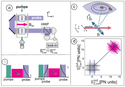
Figure 6: (a) The experimental setup is similar to the usual settings. A pulse of $B_{\text{RF}}$ at the frequency $\Omega$ is applied orthogonally to the B field, such that the created displacement in the spin lies in the same direction for both cells. (b) The pulse sequence for projection noise limited magnetometry is also similar to previous experiments. The temporal mode function for the probe is indicated as the dashed black curve. The pulse sequence to the right shows the scenario including the temporal modes for entanglement-assisted magnetometry. (c) Function principle of radio-frequency magnetometer. The atomic spin J precesses in crossed dc and rf magnetic fields (the blue dashed spiral). The state of the spin after the rf pulse (black dashed circle) is measured using a probe beam, on which the precessing J imposes oscillating polarization rotation. (d) Experimental results. Grey points are the experimental data for for the spin projection on y z plane in the rotating frame for a series of measurements of the polarization rotation signal $S_{2}^{\text{out}}(t)$ before the $B_{\text{RF}}$ is applied. The blue and the dashed black lines show the standard deviation of the total noise, and the contribution due to the projection noise (PN), respectively. The spin precession as illustrated in (c) is in corresponds to the displacement in the rotating frame indicated by the dashed blue arrow in (d). Results of the series of measurements taken with a $B_{\text{RF}}$ = 36 fT rf field applied over 15 ms are shown as pink points. The rf field is calibrated using a pick-up coil. When the entangling probe pulse is applied as explained in the text, the grey points and the pink points become correlated which leads to a reduced spin noise and improved sensitivity.

To optimize the decoherence time $T_{2}$, while the RF field is turned on, all laser fields are turned off. The pulse sequence of relevance is shown on the left of fig.6b. After the RF field, the displacement is read out via $S_{2}$ which is analyzed at the frequency $\Omega$. The measurements are weighted with suitable exponentially decaying modefunctions which give the best signal to noise ratio (SNR). In fig.6d a scatter plot of measurement outcomes for a specific realization is shown. In another setting, for $N_{A}=1.5\cdot 10^{12}$ and $\tau=22ms$ a sensitivity of $4.2(8)\cdot 10^{-16}$Tesla$/\sqrt{Hz}$ was achieved approaching the best to-date atomic rf magnetometry sensitivity lss06 obtained with $10^{4}$ times more atoms.

The achieved performance lies around 30$\%$ above the PN limit. The residual noise sources arise due to the decay of the spin and from the SN of light - which is suppressed due to the ”non-QND” type of interaction.

In earlier works JKP01 ; Quint it was shown that entanglement between two atomic ensembles can be generated via a measurement on light that has interacted with both ensembles JKP01 . In principle it should be possible to improve the sensitivity by venturing away from the CSS and towards such two mode squeezed atomic states. The drawback is that due to the short lifetimes of the squeezing compared to the optimal exposure time, the optimal setting cannot be improved in such a way. However, it is possible to improve the measurement performance for shorter RF-pulses or larger bandwidths. An additional probe pulse was used to conditionally squeeze the atomic input operators prior to the exposure to the RF field. In WJKRBP10 it was shown that an increase in the SNR can be seen for short pulses when an entangling step (see rigth pulse sequence in Fig. 6) was added.

III.4 Outlook

One future perspective of the presented setup lies in engineering miniaturized gas cells with a cross section of $200\times 200\mu$m² opening up for the possibility of smaller magnetic field sensors as well as a small fiber integrated cell network. Moving to new setup designs also gives the opportunity to decrease the effect of the main limiting factor of all presented experiments: decoherence. Here, decoherence arises amongst others from collisions with the wall, magnetic field instabilities and spontaneous emission. The resulting decay of the spin, reduces the achievable degree of entanglement, the mappping-fidelity and the sensitivity of magnetic field measurements. To diminish the effect of spontaneous emission, one approach could be the inclusion of a bad cavity around the next generation of micro cells. This enhances the collective effect on the atoms which lays the basis for all presented experiments without increasing the spontaneous emission. The effect of wall collisions can presumably be decreased by working with recently developed coatings BKLB2010 . In alkali-metal vapor cells prepared with such coatings lifetimes of the spin up to one minute have been observed.

IV Heisenberg scaling in entanglement assisted atomic metrology

Atoms of an ensemble in a spin squeezed state (SSS) are entangled  SoDCZ00 if $(\delta J_{z})^{2}<\frac{|\langle J\rangle|^{2}}{N_{A}}\Rightarrow\xi\equiv\frac{(\delta J_{z})^{2}}{|\langle J\rangle|^{2}}N_{A}<1$ where $J_{z}$ is one of the collective (quasi)-spin components orthogonal to the mean spin direction and $\xi$ defines the squeezing parameter. Under this condition the state also improves the signal-to-noise ratio in atom interferometry, metrology and sensing  WINELAND1992 .

Generation of such SSS fulfilling the above condition in an ensemble of $\sim 10^{5}$ atoms via a QND measurement of $J_{z}$. was reported in  AWO09 . The quasi-spin corresponded to the two clock levels of Cs atoms. Later it was shown that this SSS improves the precision of an atomic clock  clock2010 . As discussed in  Saffman2008 , the degree of spin squeezing scales with the optical depth $d=\sigma_{0}N_{A}/\mathcal{A}$ (with scattering cross section on resonance $\sigma_{0}$, number of atoms $N_{A}$, and beam cross section $\mathcal{A}$) as $\xi=(1/(1+d\eta)+a\eta)/(1-\eta)^{2}$ where $\eta$ is the probability of spontaneous emission caused by the QND measurement. The first term in paranthesis describes the $J_{z}$ noise reduction due to the QND measurement, the second term describes the change in the $J_{z}$ component due to the spontaneous emission and the factor $(1-\eta)$ is responsible for the shortening of the macroscopic spin due to the spontaneous emission. The constant $a$ depends on the particular level scheme and details of the QND interaction.

The QND measurement of the clock state population difference in  AWO09 is realized by detecting the state dependent phase shift of two off-resonant probe laser beams using a Mach-Zehnder interferometer. One probe $P_{\downarrow}$ is coupled to the state $|{\downarrow}\rangle\equiv 6S_{1/2}(F=3,m_{F}=0)$, while a second probe $P_{\uparrow}$ is coupled to the state $|{\uparrow}\rangle\equiv 6S_{1/2}(F=4,m_{F}=0)$ (see Fig. 7B). Cold Cs atoms are loaded into an optical dipole trap, aligned to overlap with the probe arm of the MZI, and a CSS $\bigotimes_{i=1}^{N_{A}}\left[\frac{1}{\sqrt{2}}\bigl{(}|{\downarrow}\rangle+|{\uparrow}\rangle\bigr{)}\right]_{i}$ is prepared. Successive QND measurements on the sample are performed, after which all atoms are pumped into the $F=4$ level to determine the total atom number $N_{A}$. The sequence is repeated several thousand times for various $N_{A}$.

The dichomatic QND measurement with cyclic transitions does not add any noise to $\delta J_{z}^{2}$ as elaborated in Saffman2008 which corresponds to $a=0$ in the expression for $\xi$. Hence the optimal squeezing $\xi_{\min}\propto 1/\sqrt{N_{A}}$ is expected for $\eta=\frac{1}{3}$, assuming a large resonant optical depth $d_{0}$ where $N_{A}$ is the number of atoms. The precision of the determination of the macroscopic spin direction then scales as $\delta J_{z}/(J)\propto\sqrt{\xi/N_{A}}\propto(1/N_{A})$ which is the Heisenberg scaling.

Fig. 7 demonstrates approaching the Heisenberg scaling. The atomic spin noise of the SSS becomes independent of the $N_{A}$ for large atomic numbers, the feature that ensures Heisenberg scaling for the precision of the spin direction $\delta J_{z}/(J)$.

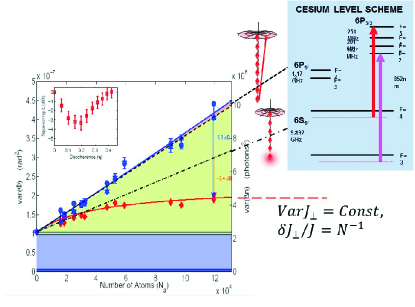
Figure 7: Blue points, stars and dashed line: Variances $\mathrm{var}(\phi_{1})$, $\mathrm{var}(\phi_{2})$ of the $J_{z}$ spin noise variance of atoms in a CSS proportional to $N_{A}$ . Dash-dotted line: equivalent CSS projection noise reduced by the loss of atomic coherence. Red diamonds and red line: reduced noise of SSS which asymptotically approaches a constant level independent of the number of atoms. Blue fields: optical shot noise (light blue) and detector noise (dark blue). Inset, Atomic level scheme and two QND probes.

V Interface to solids

In this last section we will turn to yet another avenue which is opening up for experiments with room temperature vapors of neutral atoms, and the perspective for quantum information processing associated to it. This avenue promises to lead to the integration of the Faraday based light matter interface to solid state systems, in particular to hybrid quantum systems Wallquist2009 of atomic ensembles and micro- or nanomechanical oscillators. The coupling of the latter systems to light has recently become the focus of the burgeoning field of optomechanics. Strong light-matter coupling GROEBLACHER1992 and optical cooling of mechanical oscillators close to their ground states GROEBLACHER1992 have been seen in recent experiments. For recent reviews on this field see AspelmeyerReview .

The physics of an optomechanical system can be understood from the simple picture of a harmonically bound, moving mirror, which provides one end mirror of a Fabry-Perot cavity. Small displacements of the mirror from its equilibrium position will result in phase shifts of the cavity field, i.e. shifts of the phase quadrature $p_{c}$ depending on the mirror position $x_{m}$ FootnoteMirror . In turn, the radiation pressure force will change the mirror momentum, which amounts to a change of the mechanical momentum $p_{m}$ depending on the cavity’s amplitude quadrature $x_{c}$. In a picture where only linear effects of this mutual changes are considered, we see that the resulting dynamics can be described by relations similar to the ones given in Equations (II.3.1) with $x_{A(L)},~{}p_{A(L)}$ being replaced by $p_{c(m)},~{}x_{c(m)}$ respectively. In the bad cavity limit, where the intracavity field can be adiabatically eliminated from the dynamics this statement will just as well hold true for the mechanical quadratures and the quadratures for a propagating pulse being reflected off the optomechanical system. This reasoning so far neglects the free oscillatory motion of the harmonically bound mirror at frequency $\omega_{m}$. In a regime where the pulse length $T$ is much shorter than a period $1/\omega_{m}$ this is well justified. The associated QND measurement of the mechanical displacement has recently been discussed in detail for a current optomechanical setup in Vanner2011 . In the other limit where $T\gg 1/\omega_{m}$ the oscillatory motion has to be taken into account and the input-output relations for the mechanical system and the propagating pulse are in fact equivalent to the ones for an atomic ensemble in a magnetic field causing a Larmor splitting of $\Omega=\omega_{m}$ interaction with a pulse in QND fashion, as given in Sec. II.3.1.

This analogy lies at the heart of the interface of atomic ensembles to solids suggested in Hammerer2009 , and will be summarized in the following. It was explained in Sec. II.3.1 how the QND interaction between an atomic spin and light can be realized. We have also seen that placing two atomic ensembles in magnetic fields will give rise to a QND interaction of light with EPR-operators associated to the transverse spin components of the two ensembles, cf. Equ. (4). The idea of the interface to solids is to apply this method to a hybrid system consisting of an atomic ensemble and an optomechanical system. While the latter necessarily has an effective positive “Larmor” frequency $\Omega=\omega_{m}>0$, the atomic ensemble can in turn be used to effectively realize a mechanical oscillator of negative mass with Larmor frequency $\Omega=-\omega_{m}$. For mechanical oscillators with typical resonance frequencies of several $100$kHz this requires only moderate magentic field strengths. Overall, when a sufficiently long light pulse interacts first with an optomechanical system and then with an atomic ensemble tuned to $\Omega=-\omega_{m}$ and in QND mode, then the overall input-output relation is given by Eqns. (4), with $x_{A,cos}=(x_{A}+p_{m})/\sqrt{2}$, $p_{A,cos}=(p_{A}-x_{m})/\sqrt{2}$ and $x_{A,sin}=(x_{A}-p_{m})/\sqrt{2}$, $p_{A,sin}=(p_{A}+x_{m})/\sqrt{2}$ describing now hybrid EPR operators involving the atomic spin quadratures $x_{A},~{}p_{A}$ and mechanical position and momentum operators $x_{m},p_{m}$. A homodyne measurement of of light will then project the hybrid system in an entangled EPR state, which can in principle serve as a resource for teleportation protocols.

The important point made in the original proposal Hammerer2009 was to show that the parameters of these two very different systems – a nanomechanical oscillator and a collective atomic spin – can be matched in such a way that it becomes possible to establish an interface in the sense described above. Apart from matching Larmor to mechanical resonance frequencies this requires also that the optomechanical coupling strength can be of similar magnitude than the one of the light atoms interface. We have seen that in the latter system it is essentially only the parameter $\kappa$ which enters the input output relations. In the optomechanical system the equivalent parameter turns out to be

$$\kappa_{OM}=2kx_{ZPF}\sqrt{N_{ph}}\mathcal{F},$$

where $k$ is the wave number, $x_{ZPF}=\sqrt{\hbar/2m\omega_{m}}$ the zero point fluctuation of the mechanical oscillator, $N_{ph}$ the number of photons and $\mathcal{F}$ the cavity finesse of the optomechanical system. In Hammerer2009 , we demonstrated that it is possible to have $\kappa_{OM}\simeq\kappa\simeq 1$ under compatible experimental conditions.

One major difference of the mechanical system as compared to the atomic spin is of course that the preparation of the ground state can be achieved very efficiently in atoms via optical pumping while it is a much more demanding task on the side of the mechanical oscillator. While these systems can provide very high quality factors $Q=\omega_{m}/\gamma$ on the order of $10^{6}$ (with $\gamma$ the width of the mechanical resonance), there is still a rather large mean occupation $\bar{n}=k_{B}T_{0}/\hbar\omega_{m}$ in thermal equilibrium at ambient temperature $T_{0}$, and associated to it a comparatively large thermal decoherence rate $\gamma\bar{n}$. It turns out that the protocol described above is remarkably resilient to the initial thermal occupation of the mechanical oscillator. For an initial thermal occupation $\bar{n}$ homodyne detection of $x_{L_{0},cos}^{out}$ and $x_{L_{0},sin}^{out}$ will prepare an EPR squeezed state with reduced EPR variance

$$\Delta\left(p_{A,cos}^{out}\right)^{2}+\Delta\left(p_{A,sin}^{out}\right)^{2}=\left[\frac{1}{1+\bar{n}}+2\kappa^{2}\right]^{-1}.$$

An entangled state will be produced if the right hand side falls below one, which can be achieved for moderate values of $\kappa$ even for mean initial occupations much larger than one. This can be understood by noting that – for large $\kappa$ – entanglement is here created in a projective measurement, such that the initial state and its entropy become irrelevant for a suffiently strong QND measurement. The state thus created opens an EPR channel of entanglement between optomechanics and atomic spins, a basis for quantum state transmission or transduction Rabl2009 ; Stannigel2010 .

Overall, it is remarkable to see that these very disparate systems realize very similar physics in that the light matter interaction is described by the same equations. Moreover, also the time scales of the dynamics in both systems can be comparable and are compatible for combination and interfacing. Other possible realizations of such ideas were worked out in Hammerer2009b ,Wallquist2010 and Hammerer2010b . Note that micro- and nanomechanical systems can not only be coupled to atoms, as demonstrated here, but also to many other systems, such as e.g. spin impurities, electrical (superconducting) circuits etc. Rabl2009 ; Stannigel2010 . In the long run we thus expect that these systems can play an important role as transducers for quantum information in architectures for quantum information processing.

VI Conclusions

We have reviewed the recent developments in the light-matter interface based on the Faraday interaction of light with room temperature atomic vapors. These developments are largely based on an extension of this dynamics from the well known and established QND interaction to a regime of more general interaction with a tunable balance between the components of a passive beam splitter and an active down conversion dynamics. The realization of improved magnetometry, quantum memory for squeezed state and the preparation of steady state entanglement by dissipative dynamics are all based on this tunability of the Faraday interaction. We also reviewed possible combinations and interfaces of collective atomic spins with nano- or micromechanical oscillators, providing a link between atomic and solid state physics approaches towards quantum information processing.

In the past decade quantum interfaces between neutral room temperature objects and optical photons have been extensively explored by a number of leading groups. Quantum state transfer between light and atoms, such as quantum memory and quantum teleportation, entanglement of massive objects, as well as measurements and sensing beyond standard quantum limits have been demonstrated. One promising direction for the future developments in this field is to develop a robust, integrated and scalable room temperature atom-light interface and to incorporate it into a hybrid multi-facet quantum network with other relevant quantum systems, such as nano-mechanical oscillators and electronic circuits. Micro-size room temperature atomic quantum memories in spin protecting micro-cells appear to be excellent candidates for this task. This research thus adds to the highly interdisciplinary effort to enable large scale quantum information processing, be it for long distance quantum communication, distributed quantum computation or scalable photonic quantum computers.

- (1) H. P. Specht, C. Nolleke,A. Reiserer, M. Upphoff, E. Figueroa, S. Ritter, G. Rempe, Nature 473, 190 (2011).
- (2) H. de Riedmatten, M. Afzelius, M. U. Staudt, C. Simon, G. Gisin, Nature 456 773 (2008).
- (3) M. Hedges, P. Longdell, J. Jevon, Y. Li, M. J. Sellars, Nature 465 1052 (2010).
- (4) I. Usmani, M. Afzelius, H. de Riedmatten, N. Gisin, Nat. Commun. 1, 12 (2010).
- (5) E. Saglamyurek, N. Sinclair, J. Jin, J. A. Slater, D. Oblak, F. Bussieres, M George, R. Ricken, W. Sohler, W. Tittel, Wolfgang, Nature 469, 512 (2011).
- (6) J. Cviklinski, J. Ortalo, J. Laurat, A. Bramati, M. Pinard, E. Giacobino, Phys. Rev. Lett. 101, 133601 (2008).
- (7) Z. Yuan, Y. Chen, B. Zhao, S. Chen, J. Schmiedmayer, J. Pan, Nature 454, 1098 (2008).
- (8) R. Zhao, Y. Dudin, S. Jenkins, C. Campbell, D. Matsukevich, T. Kennedy, A. Kuzmich, Nature Phys. 5, 100 (2009).
- (9) R. Zhang, S. Garner, L. Hau, Phys. Rev. Lett. 103, 233602 (2009).
- (10) B. Zhao, Y. Chen, X. Bao, T. Strassel, C. Chuu, X. Jin, J. Schmiedmayer, Z. Yuan, S. Chen, J. Pan, Nature Phys. 5, 95 (2009).
- (11) U. Schnorrberger, J. Thompson, S. Trotzky, R. Pugatch, N. Davidson, S. Kuhr, I. Bloch, Phys. Rev. Lett. 103, 033003 (2009).
- (12) K. Reim, J. Nunn, V. Lorenz, B. Sussman, K. Lee, N. Langford, D. Jaksch, I. Walmsley, Nat. Photon. 4, 218 (2010).
- (13) A. Radnaev, Y. Dudin, R. Zhao, H. Jen, S. Jenkins, A. Kuzmich, T. Kennedy, Nature Phys. 6, 894 (2010).
- (14) K. Choi, A. Goban, S. Papp, S. van Enk, H. Kimble, Nature 468, 412 (2010).
- (15) M. Hosseini, B. Sparkes, G. Campbell, P. Lam, B. Buchler, Nat. Commun. 2 174 (2011).
- (16) W. Wasilewski, T. Fernholz, K. Jensen, L.S. Madsen, H. Krauter, C. Muschik, E.S. Polzik, Opt. Express 16, 14444 (2010).
- (17) K. Jensen, W. Wasilewski, H. Krauter, T. Fernholz, B.M. Nielsen, M. Owari, M.B. Plenio, A. Serafini, M.M. Wolf, E.S. Polzik, Nature Physics 7, 13 (2010).
- (18) W. Wasilewski, K. Jensen, H. Krauter, J.J. Renema, M.V. Balabas, E.S. Polzik, Phys. Rev. Lett. 104, 133601 (2010).
- (19) A. Lvovsky, B. Sanders, W. Tittel, Nat. Photon. 3, 706 (2009).
- (20) K. Hammerer, A.S. Sørensen, E.S. Polzik, Rev. Mod. Phys. 82, 1041 (2010).
- (21) N. Sangouard, C. Simon, H. de Riedmatten, N. Gisin, Rev. Mod. Phys. 83, 33 (2011).
- (22) J. Miller, Phys. Today 63, 13 (2010).
- (23) B. Julsgaard, J. Sherson, J.I. Cirac, J. Fiurášek, E.S. Polzik, Nature 432, 482 (2004).
- (24) J.F. Sherson, H. Krauter, R.K. Olsson, B. Julsgaard, K. Hammerer, I. Cirac, E.S. Polzik, Nature 443, 557 (2006).
- (25) B. Julsgaard, A. Kozhekin, E.S. Polzik, Nature 413, 400 (2001).
- (26) , where is the creation operator for a photon with wave vector , is the speed of light, and and are the bandwidth and central frequency of the applied laser field. , where the deltafunction has a width of the order SiD03 ; MaM04 ; HaPC05 ; Hammerer2010 .
- (27) T. Holstein, H. Primakoff, Phys. Rev. 58, 1098 (1940).
- (28) Here and in the following, Gaussian input states and Gaussian measurements (homodyne detection on the quadratures of the light field) are considered. The time evolution according to a quadratic Hamiltonian is a linear transformation which preserves the Gaussian character of the involved quantum states. Therefore, the setting under consideration can be conveniently described using the Gaussian formalism.
- (29) S. Lloyd, S.L. Braunstein, Phys. Rev. Lett. 82, 1784 (1999).
- (30) B. Kraus, K. Hammerer, G. Giedke, J.I. Cirac, Phys. Rev. A 67, 42314 (2003).
- (31) We assume here a pointlike atomic ensemble located at .
- (32) D.V. Kupriyanov, O.S. Mishina, I.M. Sokolov, B. Julsgaard, E.S. Polzik, Phys. Rev. A 71, 032348 (2005).
- (33) O. Mishina, D. Kupriyanov, E.S. Polzik, in Proceedings of the NATO Advanced Research Workshop, Crete 2005: Quantum Communication and Security, vol. 199 (ISO Press, Amsterdam, 2006), vol. 199, p. 346
- (34) O.S. Mishina, D.V. Kupriyanov, J.H. Müller, E.S. Polzik, Phys. Rev. A 75, 042326 (2007).
- (35) The quantization axis is defined by the direction of the magnetic field. Therefore, we use here quantization along .
- (36) is proportional to the intensity of the applied laser light and independent of the excited state of the atomic transition driven by this field.
- (37) , where and are the atomic vector and tensor polarizabilities WFJM09 . The calculation of these values can be found for example in Hammerer2010 .
- (38) , where is the natural line width, is the photon flux per unit time, is the cross section of the applied light beam, is the wave length and is the detuning.
- (39) K. Hammerer, E.S. Polzik, J.I. Cirac, Phys. Rev. A 72, 052313 (2005).
- (40) B. Julsgaard, Entanglement and quantum interactions with macroscopic gas samples. Ph.D. thesis, University of Aarhus (2003)
- (41) K. Hammerer, E.S. Polzik, J.I. Cirac, Phys. Rev. A 74, 064301 (2006).
- (42) J. Fiurášek, J. Sherson, T. Opatrný, E.S. Polzik, Phys. Rev. A 73, 022331 (2006).
- (43) C.A. Muschik, K. Hammerer, E.S. Polzik, J.I. Cirac, Phys. Rev. A 73, 062329 (2006).
- (44) J.F. Sherson, K. Mølmer, Phys. Rev. Lett. 97(14), 143602 (2006).
- (45) H. Krauter, C.A. Muschik, K. Jensen, W. Wasilewski, J.M. Petersen, J.I. Cirac, E.S. Polzik, arXiv:1006.4344 (2010).
- (46) C.A. Muschik, E.S. Polzik, J.I. Cirac, Phys. Rev. A 83, 052312 (2011).
- (47) L.M. Duan, M.D. Lukin, J.I. Cirac, P. Zoller, Nature 414, 413 (2001).
- (48) H. Kimble, Nature 453, 1023 (2008).
- (49) Note that standard protocols such as the DLCZ scheme DLCZ01 would yield a separable mixed state if the measurement outcome is unknown or discarded.
- (50) As above, an idealized situation in a simplified model is considered. A detailed discussion including the effects of a finite optical depth and atomic motion can be found in EbDtheory ; EbDExperiment .
- (51) The definition of the operators and differs from the definition used in EbDtheory , since the atomic states for the second ensemble are defined differently (here, and , while and is used in EbDtheory ).
- (52) To this end, a sequence of infinitesimal pulses which interact with the ensembles and are subject to continuous measurements is considered. By averaging over the measurement results, the master equation is obtained.
- (53) Since the ensembles are antiparallel oriented, and .
- (54) D. DiVincenzo, Fortschr. Phys. 48, 771 (2000).
- (55) K. Honda, D. Akamatsu, M. Arikawa, Y. Yokoi, K. Akiba, S. Nagatsuka, T. Tanimura, A. Furusawa, M. Kozuma, Phys. Rev. Lett. 100, 093601 (2008).
- (56) J. Appel, E. Figueroa, D. Korystov, M. Lobino, A. Lvovsky, Phys. Rev. Lett. 100, 093602(2008).
- (57) C.W. Chou, H. de Riedmatten, D. Felinto, S.V. Polyakov, S.J. van Enk, H.J. Kimble, Nature 438, 828 (2005).
- (58) M. Eisaman, A. André, F. Massou, M. Fleischhauer, A. Zibrov, M.D. Lukin, Nature 438, 837 (2005).
- (59) D.N. Matsukevich, T. Chanelière, S.D. Jenkins, S.Y. Lan, T.A.B. Kennedy, A. Kuzmich, Phys. Rev. Lett. 96, 030405 (2006).
- (60) Z.S. Yuan, Y.A. Chen, B. Zhao, S. Chen, J. Schmiedmayer, J.W. Pan, Nature 454, 1098 (2008).
- (61) J. Appel, P. Windpassinger, D. Oblak, U. Hoff, N. Kjærgaard, E. Polzik, PNAS 106, 10960 (2009).
- (62) C. Gross, T. Zibold, E. Nicklas, J. Esteve, M.K. Oberthaler, Nature 464, 1165 (2010).
- (63) M.F. Riedel, P. Böhi, Y. Li, T.W. Hänsch, A. Sinatra, P. Treutlein, Nature 464, 1170 (2010).
- (64) T. Fernholz, H. Krauter, K. Jensen, J.F. Sherson, A.S. Sørensen, E.S. Polzik, Phys. Rev. Lett. 101, 073601 (2008).
- (65) M.B. Plenio, S.F. Huelga, Phys. Rev. Lett. 88, 197901 (2002).
- (66) B. Kraus, J.I. Cirac, Phys. Rev. Lett. 92, 013602 (2004).
- (67) S. Diehl, A. Micheli, A. Kantian, B. Kraus, H.P. Büchler, P. Zoller, Nature Physics 4, 878 (2008).
- (68) F. Verstraete, M.M. Wolf, J.I. Cirac, Nature Physics 5, 633 (2009).
- (69) J.T. Barreiro, M. Müller, P. Schindler, D. Nigg, T. Monz, M. Chwalla, M. Hennrich, C.F. Roos, P. Zoller, R. Blatt, Nature 470, 486 (2011).
- (70) H. Krauter, C.A. Muschik, K. Jensen, W. Wasilewski, J. M. Petersen, J. I. Cirac, E. S. Polzik, Phys. Rev. Lett. 107, 080503 (2011).
- (71) C. Schori, J.L. Sørensen, E.S. Polzik, Phys. Rev. A 66, 033802 (2002).
- (72) M. Balabas, T. Karaulanov, M. Ledbetter, D. Budker, Phys. Rev. Lett. 105, 070801 (2010).
- (73) D. Budker, M. Romalis, Nature Phys. 3, 227 (2007).
- (74) M. Tsang, H.M. Wiseman, C.M. Caves, Phys. Rev. Lett. 106, 090401 (2011).
- (75) D.J. Wineland, J.J. Bollinger, W.M. Itano, F.L. Moore, D.J. Heinzen, Phys. Rev. A 46, R6797 (1992).
- (76) S. Lee, K. Sauer, S. Seltzer, O. Alem, M. Romalis, Appl. Phys. Lett. 89, 214106 (2006).
- (77) J. Sherson, B. Julsgaard, E. Polzik, Advances in Atomic, Molecular, and Optical Physics 54 (2006).
- (78) A. Sørensen, L.M. Duan, J. Cirac, P. Zoller, Nature 409, 63 (2001).
- (79) D.J. Wineland, J.J. Bollinger, W.M. Itano, F.L. Moore, D.J. Heinzen, Phys. Rev. A 46, R6797 (1992).
- (80) A. Louchet-Chauvet, J.J.R. J. Appel, D. Oblak, N. Kjaergaard, E.S. Polzik, New J. Phys 12, 065032 (2010).
- (81) M. Saffman, D. Oblak, J. Appel, E.S. Polzik, Phys. Rev. A 79, 023831 (2009).
- (82) M. Wallquist, K. Hammerer, P. Rabl, M. Lukin, P. Zoller, Physica Scripta T137, 014001 (2009).
- (83) S. Groblacher, K. Hammerer, M. Vanner, M. Aspelmeyer, Nature 460, 724 (2009).
- (84) M. Aspelmeyer, S. Gröblacher, K. Hammerer, , N. Kiesel, JOSA B 27, A189 (2010).
- (85) We assume the canonical conjugate operators for the mechanical system to be dimensionless .
- (86) M.R. Vanner, I. Pikovski, M.S. Kim, C. Brukner, K. Hammerer, G.J. Milburn, M. Aspelmeyer, arXiv:1011.0879 (2011).
- (87) K. Hammerer, M. Aspelmeyer, E.S. Polzik, P. Zoller, Phys. Rev. Lett. 102, 020501 (2009).
- (88) P. Rabl, P. Cappellaro, M. M. Dutt, L. Jiang, J. Maze, M. Lukin, Phys. Rev. B 79, 041302 (2009).
- (89) K. Stannigel, P. Rabl, A. Sørensen, P. Zoller, M. Lukin, Phys. Rev. Lett. 105, 220501 (2010).
- (90) K. Hammerer, M. Wallquist, C. Genes, M. Ludwig, F. Marquardt, P. Treutlein, P. Zoller, J. Ye, H.J. Kimble, Phys. Rev. Lett. 103, 063005 (2009).
- (91) M. Wallquist, K. Hammerer, P. Zoller, C. Genes, M. Ludwig, F. Marquardt, P. Treutlein, J. Ye, H.J. Kimble, Phys. Rev. A 81, 023816 (2010).
- (92) K. Hammerer, K. Stannigel, C. Genes, P. Zoller, P. Treutlein, S. Camerer, D. Hunger, T.W. Hänsch, Phys. Rev. A 82, 021803 (2010).
- (93) A. Silberfarb, I. Deutsch, Phys. Rev. A 68, 13817 (2003).
- (94) L. Madsen, K. Mølmer, Phys. Rev. A 70, 52324 (2004).