Scattering of evanescent wave by two cylinders
near a flat boundary

Abstract

Two-dimensional problem of evanescent wave scattering by dielectric or metallic cylinders near the interface between two dielectric media is solved numerically by boundary integral equations method. A special Green function was proposed to avoid the infinite integration. A pattern with a circular and a prolate elliptic cylinders, respectively, is suggested to simulate the sample and the probe in near-field optical microscopy. The energy flux in the midplane of the probe-cylinder is calculated as a function of its position.

The diffraction limit in optics, known to originate from the wave nature of light, gives a striking example of a physical restriction being a target of increasing efforts to overcome. More than a century ago it was realized that the wavelength limits the smallest spot within the electromagnetic energy can be localized, as well as the smallest details one can optically resolve are comparable to the wavelength. However, further study showed that these obstacles, in fact, concern a traveling (homogeneous) electromagnetic wave. Unlike, the inhomogeneous (also referred to as evanescent) waves, which can not propagate far away from their source, open the way to clear up the limitations due to diffraction and go towards the optics of tiny objects. For instance, the nanosized highly-polarizable (i.e. metal) particles well manage to concentrate the light energy within few nanometer range [1]. A near-field scanning optical microscopy (NSOM) was suggested to obtain optical signal from the objects at nanoscale (see [2, 3] and references therein) using sharp tips; the latter serve much like an optical antenna [4], which receives the energy of the local field and then transfers it to a detector. Thus, the nanophotonics is, basically, an optics of evanescent waves, and, consequently, the fundamental optical processes (such as diffraction, interference, scattering) are to be reconsidered.

In past two decades a substantial progress is achieved in nano-optics [5, 6]. However, a significant methodological deficiency persists even for the plain, basic problems, like scattering of the evanescent wave by a body. The trouble is that evanescent wave can not be considered in isolation from its source (for instance, the interface where the total internal reflection takes place), therefore the source is certainly affected by the scatterer as being located within a few wavelengths. In paper [7] the general analytical approach is suggested that makes possible to do very effective calculations of the evanescent wave scattering on a 2D particle (a cylinder) near a flat boundary. In the present work we make the next step and consider the problem of two optically coupled objects placed into the inhomogeneous wave. Our main goal is to get a physical insight into the near-field scanning optical microscopy, which minimally involves two small bodies — the studied object and the probe. We believe our work is a useful starting point for analysis of particular NSOM schemes which will allow for correct extraction of the near field and structural information from NSOM data. Keeping in mind this application to the realistic configurations, we should focus our attention on the first-principles approaches, avoiding restricting assumptions and approximations.

We start from the Helmholtz equation

$$(\bigtriangleup+k^{2})\mathscr{H}=0,$$ (1)

where $\bigtriangleup$ is the Laplace operator, $\mathbf{k}$ is the wavevector. Consider domain $\mathscr{D}$ with permittivity $\varepsilon_{\textrm{in}}$ and its boundary $\Gamma=\partial\mathscr{D}$. Denote $\varepsilon_{\textrm{out}}$ the permittivity of exterior of $\mathscr{D}$. The Green theorem can be written inside and outside domain $\mathcal{D}$, respectively

$$\mathscr{H}(\mathbf{r})=-\oint_{\Gamma}\left(\frac{\partial g}{\partial n^{\prime}}\mathscr{H}^{\prime}-g\frac{\partial\mathscr{H}^{\prime}}{\partial n^{\prime}}\right)\,ds^{\prime},$$ (2)

$$\mathscr{H}(\mathbf{r})=\oint_{\Gamma}\left(\frac{\partial g}{\partial n^{\prime}}\mathscr{H}^{\prime}-g\frac{\partial\mathscr{H}^{\prime}}{\partial n^{\prime}}\right)\,ds^{\prime}+\mathscr{H}_{0}(\mathbf{r}).$$ (3)

Here $\mathbf{r}\notin\Gamma$, $\mathscr{H}^{\prime}\equiv\mathscr{H}(\mathbf{r}^{\prime})$, $\partial/\partial n^{\prime}$ is the derivative along the internal normal, $g(\mathbf{r},\mathbf{r}\,^{\prime})$ is a fundamental solution to the inhomogeneous Helmholtz equation

$$(\bigtriangleup+k^{2})g=\delta(x-x^{\prime})\delta(y-y^{\prime}).$$ (4)

It should be noted that function $g(\mathbf{r},\mathbf{r}\,^{\prime})$ is not fully arbitrary, namely, should satisfy the radiation condition. Hence, the implicit integral over an infinitely remote contour in Eq. 3 reduces to the field in the absence of scatterer $\mathscr{D}$, denoted as $\mathscr{H}_{0}$.

Let us consider TM wave for which $\mathscr{H}$ is the magnetic field. It has to satisfy boundary conditions for the field and its normal derivative

$$\left[\mathscr{H}\right]_{\Gamma}=\left[\frac{1}{\varepsilon}\frac{\partial\mathscr{H}}{\partial n}\right]_{\Gamma}=0,$$ (5)

where square brackets denote the jump, $\varepsilon$ corresponds to either $\varepsilon_{\rm in}$ or $\varepsilon_{\rm out}$. Conditions (5) mean that the magnetic field is always continuous at $\Gamma$, whereas its normal derivative has a jump depending on $\varepsilon_{\rm in}$, $\varepsilon_{\rm out}$.

In order to find the field with the help of the Green theorem (2), (3) we need to know $\mathscr{H}$ and $\partial\mathscr{H}/\partial n$ at boundary $\Gamma$. These two independent functions satisfy the following coupled equations at $\mathbf{r}\in\Gamma$:

$$\frac{1}{2}\mathscr{H}(\mathbf{r})=-\oint_{\Gamma}\left(\frac{\partial g_{\textrm{in}}}{\partial n^{\prime}}\mathscr{H}^{\prime}-g_{\textrm{in}}\frac{\varepsilon_{\textrm{in}}}{\varepsilon_{\textrm{out}}}\frac{\partial\mathscr{H}^{\prime}}{\partial n^{\prime}}\right)\,ds^{\prime},$$ (6)

$$\frac{1}{2}\mathscr{H}(\mathbf{r})=\oint_{\Gamma}\left(\frac{\partial g_{\textrm{out}}}{\partial n^{\prime}}\mathscr{H}^{\prime}-g_{\textrm{out}}\frac{\partial\mathscr{H}^{\prime}}{\partial n^{\prime}}\right)\,ds^{\prime}+\mathscr{H}_{0}(\mathbf{r}),$$ (7)

which are obtained by approaching $\Gamma$ from either inner or outer domains. Here the fundamental solution inside and outside $\mathscr{D}$ is denoted as $g_{\textrm{in}}$ and $g_{\textrm{out}}$, respectively.

After solving coupled integral equations (6), (7) the field in arbitrary point can be calculated using (2), (3). This approach is the base for the boundary element method (BEM) [8, 9]. Its advantage consists in diminishing the problem dimension. For instance, in two-dimensional geometry the method deals with one-dimensional contour $\Gamma$, and then occurs to be very fast and accurate. The method could be extended to several domains. For this purpose we must consider integration (6), (7) along an unlinked manifold $\Gamma$ with corresponding fundamental solution $g_{\textrm{in}}$ inside each. External function $g_{\textrm{out}}$ should satisfy the Sommerfeld radiation condition at infinity, i.e. be the diverging spherical or cylindrical wave.

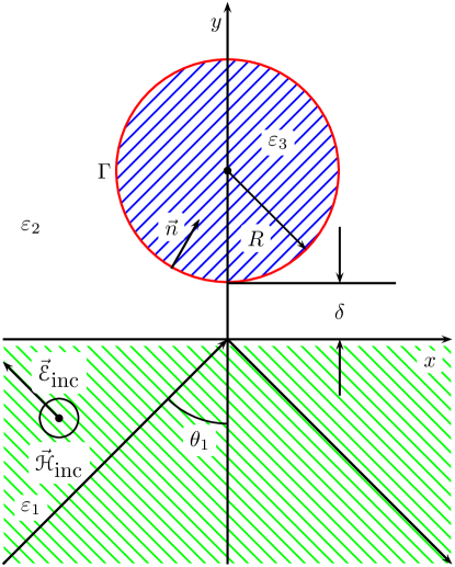
Figure 1: The geometry of light scattering.

We consider an evanescent wave, Fig. 1. The plane running wave $\mbox{$\mathscr{H}$}(\mathbf{r},t)=\mbox{$\mathscr{H}$}_{\textrm{inc}}\exp\left(-i\omega t+i\mathbf{k}_{1}\cdot\mathbf{r}\right)$ goes from the dielectric media $\varepsilon_{1}$ to other medium with permittivity $\varepsilon_{2}$; $\theta_{1}$ is the incident angle between the wavevector $\mathbf{k}_{1}$ and the normal to the boundary. While it is greater than $\theta_{0}=\arcsin\sqrt{{\varepsilon_{2}}/{\varepsilon_{1}}}$, the angle of the total internal reflection, only the evanescent wave with coordinate dependence $\exp(-\kappa y+ik_{2x}x)$ penetrates into medium 2, where

$$\kappa=\frac{\omega}{c}\sqrt{\varepsilon_{1}\sin^{2}\theta_{1}-\varepsilon_{2}},\quad k_{2x}=k_{1x}=\frac{\omega}{c}\sqrt{\varepsilon_{1}}\sin\theta_{1},$$ (8)

$\omega,c$ are the frequency and speed of light.

Two independent polarization states of falling wave are possible. We consider TM-wave with magnetic field vector perpendicular to the plane of incidence. This case is more interesting in view of the plasmon resonances study, since electric field vector lies in $xy$ plane where the cylinder has a finite size. The solution for TE-wave can be considered in the same way. The magnetic field of the wave obeys the Helmholtz equation (1), then the BEM method is applicable. However, the problem arises with the infinite integration path along $x$-axis that is hard for numerical calculation.

To avoid this difficulty we look for the specific Green function $G(x,y;x^{\prime},y^{\prime})$ satisfying inhomogeneous equation (4) in media 1 and 2. Function $G$ depends on difference $x-x^{\prime}$ only, due to translational symmetry. The boundary condition at $y=0$ is

$$\left[G(x,y;x^{\prime},y^{\prime})\right]_{y=0}=\left[\frac{1}{\varepsilon}\frac{\partial G(x,y;x^{\prime},y^{\prime})}{\partial y}\right]_{y=0}=0.$$ (9)

After the Fourier transformation

$$G(x,y;0,y^{\prime})=\frac{1}{2\pi}\int_{-\infty}^{\infty}G_{q}(y,y^{\prime})e^{iqx}\,{dq}$$ (10)

Eq. (4) is reduced to an ordinary differential equation having exponential solutions. Using conditions (9) we obtain the function at $y^{\prime}>0$ in $q$-domain

$$G_{q}=-\frac{1}{2\mu_{2}}\begin{cases}\left[1+r(q)\right]e^{\mu_{1}y-\mu_{2}y^{\prime}},&y<0,\\ e^{-\mu_{2}|y-y^{\prime}|}+r(q)e^{-\mu_{2}|y+y^{\prime}|},&y>0.\end{cases}$$ (11)

Here $r(q)=(\varepsilon_{1}\mu_{2}-\varepsilon_{2}\mu_{1})/(\varepsilon_{1}\mu_{2}+\varepsilon_{2}\mu_{1})$ is the Fresnel reflection coefficient of $p$-wave at normal incidence [10], $\mu_{1,2}^{2}=q^{2}-k_{1,2}^{2}$. Carrying out Fourier transformation (10) of function (11) at $y>0$ we have two terms

$$G_{1}=-\int\limits_{-\infty+i0}^{\infty-i0}e^{-\mu_{2}|y-y^{\prime}|+iq(x-x^{\prime})}\frac{dq}{4\pi\mu_{2}},$$ (12)

$$G_{2}=-\int\limits_{-\infty+i0}^{\infty-i0}e^{-\mu_{2}|y+y^{\prime}|+iq(x-x^{\prime})}\frac{r(q)\,dq}{4\pi\mu_{2}}.$$ (13)

and $G=G_{1}+G_{2}$, where the sign of square root is given by the rule $\sqrt{q^{2}-k_{2}^{2}}\to-i\sqrt{k_{2}^{2}-q^{2}},q^{2}<k_{2}^{2}$.

The first term (12) can be calculated analytically and reduces to the Green function in the homogeneous space

$$G_{1}(\mathbf{r};\mathbf{r}\,^{\prime})=\frac{1}{4i}{H_{0}^{(1)}\left(k_{2}\rho_{-}\right)},$$ (14)

where $H_{0}^{(1)}$ denotes the Hankel function of the first kind [11], $\rho_{\pm}^{2}=(x-x^{\prime})^{2}+(y\pm y^{\prime})^{2}$. The second term $G_{2}$ gives the effect of the reflected image source. The amplitude of source at each $q$ is equal to the reflection coefficient $r(q)$. Thus along with the point source at $(x^{\prime},y^{\prime})$ we have to consider the mirror-image source $r(q)$ at $(x^{\prime},-y^{\prime})$. The total field at the upper half-plane is the sum of fields generated by the source and its image at each $q$. The Green function automatically takes into account the multiple scattering. The Green function of this type was studied for homogeneous waves: spherical acoustic, see [12, 13], or cylindrical electromagnetic waves [14].

The asymptotic behavior of the Green function in far field can be found by the steepest descent method [15]. The stationary point is $q_{0}=k_{2}|x-x^{\prime}|/\rho$, where $\rho=\rho_{-}$ for $G_{1}$ and $\rho=\rho_{+}$ for $G_{2}$. The result is a sum of cylindrical waves $G\propto{\rho_{-}^{-1/2}}{e^{ik_{2}\rho_{-}}}+r_{0}{\rho_{+}^{-1/2}}{e^{ik_{2}\rho_{+}}},$ where

$$r_{0}=\frac{\varepsilon_{1}\sin\varphi-\sqrt{\varepsilon_{2}(\varepsilon_{1}-\varepsilon_{2}\cos^{2}\varphi)}}{\varepsilon_{1}\sin\varphi+\sqrt{\varepsilon_{2}(\varepsilon_{1}-\varepsilon_{2}\cos^{2}\varphi)}}$$ (15)

is the reflection coefficient at $q=q_{0}$, $\varphi$ is the polar angle of observation counted out from $x$-direction. The reflection coefficient is $r_{0}=-1$ at $\varphi=0$ and $(\sqrt{\varepsilon_{1}}-\sqrt{\varepsilon_{2}})/(\sqrt{\varepsilon_{1}}+\sqrt{\varepsilon_{2}})$ at $\varphi=\pi/2$. It turns to zero at $\varphi=\arctan\sqrt{\varepsilon_{1}/\varepsilon_{2}}$, i.e. at the Brewster angle.

Green function (12), (13), exploited as the external fundamental solution for coupled integral equations (6), (7), allows us to avoid the infinite integration along axis $x$. Then we can solve the equations for two contours. The algorithm has been tested in the case of one contour and homogeneous wave when $\varepsilon_{1}=\varepsilon_{2}$. There are analytical formula for circular cylinder [16] and numerical calculations for a cylinder with elliptic cross-section [17]. Comparison demonstrates the relative consistency within $10^{-4}$ for $N=360$ panels approximating contour $\Gamma$.

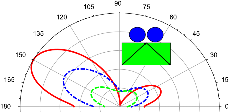
Figure 2: Energy flux through a distant semicircle (arb. units) from two equal circles with distance between centers $L=0.21~{}\mu$m as a function of polar angle $0<\varphi<\pi$ at $\lambda=1.512~{}\mu$m, $R=0.1~{}\mu$m, $\delta=0.01~{}\mu$m, $\theta_{1}=\pi/4,\varepsilon_{2}=1,\varepsilon_{3}=\varepsilon_{4}=-91.5+10.3i$, and different $\varepsilon_{1}=2$ (solid line), 2.25 (dot-dahed), 3 (dashed).

Without scattering body the electric field vector ${\mathscr{E}}$ in medium 2 has only $y$-component. The scatterer produces a small component $\mathscr{E}_{x}$ and the evanescent wave is partially converted into diverging one. The corresponding Pointing vector

$$\mathbf{S}=\frac{c}{8\pi}\textrm{Re}\,\left(\mbox{$\mathscr{E}$}\times\mbox{$\mathscr{H}$}^{*}\right)$$ (16)

acquires a nonzero $y$-component, $S_{y}$, so the energy flux outgoing from the plane interface appears. The flux of scattered wave is calculated at distance $\sim 2\lambda$, i.e. in the wave zone, and normalized by the average flux of the incoming wave in the first medium $S_{\rm inc}=c\mathscr{H}_{\rm inc}^{2}/8\pi\sqrt{\varepsilon_{1}}$. Indicatrix of the scattering into the upper half-space is shown in Fig. 2. Hereafter the insets show the configuration of scattering bodies. The scattering is minimal in normal or longitudinal direction and maximal at some medium angles. It is the quadruple contribution due to the field of image source (15) and decay of the evanescent wave amplitude with $y$. The angle $\varphi$ of the first maximum increases with $\varepsilon_{1}$. For $\varepsilon_{1}=2$ the first maximum is $23^{\circ}$ and for $\varepsilon_{1}=3$ it is $41^{\circ}$. The forward-backward asymmetry of indicatrix is a clear evidence of violation of the dipole approximation owing to finite sizes ($2kR\approx 0.8$).

\psfrag{x1}{\large$x,\mu$m}\psfrag{H}[tl][tr]{$\mathscr{H}/\mathscr{H}_{\rm inc}$}\includegraphics[width=390.25534pt]{line3}

Figure 3: The magnetic field at the bottom point of ellipse as a function of coordinate $x$ at distance $y=0.15$ from the plane (solid line). Parameters are $\lambda=1.512~{}\mu$m, $R=0.06~{}\mu$m, $\delta=0.01~{}\mu$m, $\varepsilon_{1}=\varepsilon_{3}=\varepsilon_{4}=2.25,\varepsilon_{2}=1,\theta_{1}=\pi/4$. The same without the ellipse ($\varepsilon_{4}=1$, dashed).

The method can be applied also to different cylinders. We choose the first cylinder ($\varepsilon_{\textrm{in}}=\varepsilon_{3}$) with round cross section whereas that of the second cylinder ($\varepsilon_{\textrm{in}}=\varepsilon_{4}$) is a prolate ellipse with minor semiaxis $a=0.04~{}\mu$m and axis ratio $b/a=10$. The major axis is chosen along $y$-direction. Fig. 3 shows the field near the tip as a function of coordinate $x$ at $y=0.15~{}\mu$m, when the ellipse is moving along to $x$ axis. The pattern in the near-field domain is much more complicated than in the wave zone. We see the slight low-frequency oscillations at the right side and deep high-frequency at the left. The physical nature of the oscillations consists in the interference between falling evanescent wave and the diverging wave scattered by the circle. They are counter-propagated at the left and co-propagated at the right. Their spatial frequencies are different $k_{\pm}=k_{x}\pm k_{2}$. However, in considered case $k_{x}=k_{1}\sin\theta_{1}\approx k_{2}$, then the interference oscillation at the right side has a nearly zero frequency. The slight interference pattern at the right in this case is caused by the scattering by the tip and these oscillations vanish without the tip.

\psfrag{Abs}[tr][Bl]{\large$x,\mu$m}\psfrag{Ord}[tl][Bl]{Flux}\includegraphics[width=346.89731pt]{ellipse}

Figure 4: Energy going through the central cross section in $y$-direction of the ellipse as a function of its horizontal position $x$ at distance from the plane $y=0.15$ (solid line), 0.35 (dashed), 0.50 $\mu$m (dot-dash). Parameters are $\lambda=1.512,R=0.06,\delta=0.01~{}\mu$m, $\varepsilon_{1}=\varepsilon_{3}=\varepsilon_{4}=2.25,\varepsilon_{2}=1,\theta_{1}=\pi/4$.

Fig. 4 shows the energy going along the major axis through the ellipse middle cross-section as a function of coordinate $x$, namely, the component $S_{y}$ of vector (16) averaged over the horizontal cross-section. The vertical distance of the tip from the interface is $d=0.15\div 0.50~{}\mu$m, then the minimal distance between the tip of ellipse and the circle starts from $0.02~{}\mu$m. We see interference oscillations in the coordinate dependence, the amplitude decreasing with the distance between the tip and the plane. As follows from Fourier transform (11), the higher spatial harmonics with $q^{2}>k_{2}^{2}$ decay exponentially with distance like $\exp(-\mu_{2}y)$. Then the small details are not visible in the far-field pattern. However at $ky\ll 1$ the exponent is not negligible, and then the small-scale details become apparent. The near field can be observed if one extract the signal and transfer it to the far zone. In our calculation the stretched ellipse plays a role of such a transmitter.

The energy flux through the far central plane is a simplest (two-dimensional in our case) model of NSOM [5, 2, 3]. The curves in Fig. 4 correspond to instrumental function of the microscope. Although, this statement should not be taken literally. The multiple scattering leads to back influence of the probe to the object then it is not a usual linear function of response.

The coupled boundary equations describing the scattering of the evanescent wave are solved for two cylinders. The asymmetry of indicatrix and oscillations in the coordinate dependence are observed. The BEM with proposed Green’s function is rather general and applicable for any contour $\Gamma$ or several contours. It can be extended also for 3D geometry. The Green function could find applications in other calculations, e.g. volume integral equations including the Born series and discrete dipole approximation.

Authors are grateful to E. V. Podivilov for helpful discussions. This work is supported by the Government program NSh-4339.2010.2, program # 21 of the Russian Academy of Sciences Presidium, and interdisciplinary grant #42 from the Siberian Branch of RAS.

References

- [1] M. I. Stockman, “Nanoplasmonics: The physics behind the applications,” Physics Today 64, 39–44 (2011)
- [2] Jean-Jacques Greffet and Rémi Carminati, “Image formation in near-field optics,” Progress in Surface Science 56, 133–237 (1997)
- [3] Bert Hecht, Beate Sick, Urs P. Wild, Volker Deckert, Renato Zenobi, Olivier J. F. Martin, and Dieter W. Pohl, “Scanning near-field optical microscopy with aperture probes: Fundamentals and applications,” The Journal of Chemical Physics 112, 7761–7774 (2000)
- [4] L. Novotny and N. van Hulst, “Antennas for light,” Nature Photonics 5, 83–90 (2011)
- [5] Lukas Novotny and Bert Hecht, Principles of Nano-Optics (Cambridge University Press, Cambridge — New York, 2006)
- [6] Christian Girard, “Near fields in nanostructures,” Reports on Progress in Physics 68, 1883–1933 (2005)
- [7] O. V. Belai, L. L. Frumin, S. V. Perminov, and D. A. Shapiro, “Scattering of evanescent electromagnetic waves by cylinder near flat boundary: the Green function and fast numerical method,” Opt. Lett. 36, 954—956 (2011)
- [8] D. L. Colton and Kress R., Integral equation methods in scattering theory (Wiley, New York, 1983)
- [9] C. A. Brebbia, J. C. F. Telles, and L. C. Wrobel, Boundary element techniques (Springer, Berlin, 1984)
- [10] S. G. Rautian, Introduction to physical optics (URSS, Moscow, 2009) [in Russian]
- [11] F. W. J. Ovler, D. W. Lozier, R. F. Boisvert, and C. W. Clark, NIST Handbook of Mathematical Functions (Cambridge University Press, Cambridge — New York, 2010)
- [12] L. M. Brekhovskikh, Waves in layered media (Academic Press, New York, 1980)
- [13] L. D. Landau and E. M. Lifshitz, Fluid Mechanics (Course of Theoretical Physics. Vol. 6) (Pergamon, New York, 1959)
- [14] François Pincemin, Anne Sentenac, and Jean-Jacques Greffet, “Near field scattered by a dielectric rod below a metallic surface,” J. Opt. Soc. Am. A 11, 1117–1127 (1994)
- [15] N. Bleistein and R. H. Handelsman, Asymptotic Expansion of Integrals (Dover, New York, 1986)
- [16] R. F. Harrington, Time-Harmonic Electromagnetic Fields (Wiley, NewYork, 2001)
- [17] S. V. Zymovetz and P. I. Geshev, “Boundary integral equation method for analysis of light scattering by 2d nanoparticles,” Technical Physics 51, 291–296 (2006)