Effects of the dielectric discontinuity on the counterion distribution in a colloidal suspension

Abstract

We introduce a new method for simulating colloidal suspensions with spherical colloidal particles of dielectric constant different from the surrounding medium. The method uses exact calculation of the Green function to obtain the ion-ion interaction potential in the presence of a dielectric discontinuity at the surface of the colloidal particle. The new method is orders of magnitude faster than the traditional approaches based on series expansions of the interaction potential.

I Introduction

Colloidal suspensions are of fundamental interest for various applications. One of the basic problems of colloidal science is how to stabilize a lyophobic colloidal suspension against flocculation and precipitation. A common approach is to synthesize particles with acidic or basic charged groups on the surface Miraballes-Martinez and Forcada (2000); Miraballes-Martinez et al. (2001). When placed in a polar medium such as water, these groups become ionized and the particles acquire a net charge. Repulsion between like-charged colloidal particles then prevents them from coming into a close contact where the short-range van der Waals forces become important. Addition of electrolyte to colloidal suspension leads to screening of the Coulomb repulsion Levin (2002). At critical coagulation concentration (CCC), the repulsive energy barrier disappears and the van der Waals forces drive colloidal coagulation and precipitation Lopez-Leon et al. (2003, 2008); Peula-Garcia, Ortega-Vinuesa, and Bastos-Gonzalez (2010); dos Santos and Levin (2011). It is also well known that addition of even very small amount of multivalent ions leads to a rapid precipitation. The correlation induced attraction between the colloidal particles produced by the multivalent ions is sufficient to precipitate colloidal suspensions even without taking into account the van der Waals forces. The like-charge attraction has been extensively explored in colloidal and polyelectrolyte literature Rouzina and Bloomfield (1996); Linse and Lobaskin (1999); Wu et al. (1999); Gelbart et al. (2000); Solis and de la Cruz (2001). A related phenomenon known as the charge reversal has also attracted a lot of attention over the recent years Lozada-Cassou, Saavedra-Barrera, and Henderson (1982); Pianegonda, Barbosa, and Levin (2005); Diehl and Levin (2006, 2008); Guerrero-Garcia, Gonzalez-Tovar, and de la Cruz (2010); dos Santos, Diehl, and Levin (2010). In this case electrostatic correlations result in a strong colloid-counterion associationLevin (2002). The counterion condensation can be so significant as to reverse the electrophoretic mobility of colloidal particles Quesada-Pérez, Callejas-Fernández, and Hidalgo-Álvarez (2002); Fernandez-Nieves et al. (2005).

Most of the theoretical work on stability of colloidal suspensions and the charge reversal, however, neglects the effects of the dielectric discontinuity at the particle/solvent interface. In fact, in many colloidal suspensions the static dielectric constant of colloidal particles can be $20$ to $40$ times lower than the static dielectric constant of the surrounding water. This means that an ion in the vicinity of colloidal surface will encounter a strong ion-image repulsion. This repulsion can significantly affect the effective charge of the colloid-counterion complex and thus modify the colloid-colloid interaction potential. The polarization effects, however, have been mostly neglected in almost all of the theoretical studies. The reason for this is that it is very hard to include the dielectric discontinuities in anything but the simplest planar geometry. Thus, even to perform a Monte Carlo simulation that accounts for the dielectric discontinuity requires a significant computational effort. Some years ago Linse Linse (1986) proposed to account for the induced charges by treating the low dielectric colloidal particle as if it was an “inverse” conductor. It is well known that if one places a charge near a conducting sphere, a surface charge will be induced on the sphere J. D. Jackson (1999). The field produced by the surface charge is exactly equivalent to the field produced by two point charges of opposite sign, one located at the spheres inversion point and another at its center. In the case of a conductor, the charge at the inversion point has the opposite sign to the charge placed outside the sphere, so that this charge is attracted to the conductor. Linse suggested that the low dielectric sphere in water can be treated as an inverse conductor, meaning that the same construction should apply to locate the images, but that their sign will be the opposite of the images inside the conducting sphere. This, however, is not quite right. Because of the complicated boundary conditions (BCs) imposed by the Maxwell equations at the dielectric interface, one can not satisfy the BCs with only two pointlike image charges. In fact one needs an infinite number of images Lindell (1992); Norris (1995).

Polarization effects have also been explored in ionic liquids Reed, Lanning, and Madden (2007); Reed, Madden, and Papadopoulos (2008); Loth, Skinner, and Shklovskii (2010); Outhwaite, Lamperski, and Bhuiyan (2011) and for polyelectrolyte adsorption Messina (2004, 2006); Seijo et al. (2009) in a slab geometry. In this paper we will derive the explicit inter-ionic interaction potential which very accurately accounts for the dielectric discontinuity for spherical colloidal particles. We compare our results with the Monte Carlo simulations of Messina Messina (2002), who obtained the ion-ion interaction potential as an infinite series in Legendre polynomials. In the final part of the paper we will analyze the effect of 1:1 electrolyte on the distribution of trivalent and monovalent counterions near the colloidal surface.

II Method

We will use a primitive model of a colloidal suspension in which colloidal particle is represented by a sphere of radius $a$ and the dielectric constant $\epsilon_{c}$. Water will be modeled as a uniform dielectric of permittivity $\epsilon_{w}$. The system is at room temperature, so that the Bjerrum length, defined as $\lambda_{B}=q^{2}/\epsilon_{w}k_{B}T$, is $7.14$Å. Consider an $\alpha$-valent ion of charge $Q=\alpha q$, where $q$ is the proton charge, at position ${\bf r}_{i}$ from the center of the colloidal particle. The Maxwell equations require the continuity of the tangential component of the electric field and the continuity of the normal component of the displacement field across the colloid-water interface. It is possible to show Lindell (1992); Norris (1995) that this boundary conditions can be satisfied exactly by placing an image charge $Q^{\prime}=\gamma Qa/r_{i}$ inside the colloid at the inversion point ${\bf r^{\prime}}_{i}={\bf r}_{i}a^{2}/r_{i}^{2}$ and a counterimage line-charge $\lambda(u)$, distributed along the line connecting the center of colloid with the inversion point ${\bf r^{\prime}_{i}}$, with line-charge density

$$\lambda(u)=-\dfrac{Q^{\prime}(1+\gamma)}{2r^{\prime}_{i}}\left(\dfrac{u}{r^{\prime}_{i}}\right)^{\frac{\gamma-1}{2}}\ ,$$ (1)

where $\gamma=(\epsilon_{w}-\epsilon_{c})/(\epsilon_{w}+\epsilon_{c})$ and $0\leq u\leq r^{\prime}_{i}$ is the distance along the line, see Fig. 1. Note that this construction does not change the net charge of the colloidal particle, that is the total counterimage charge is $-Q^{\prime}$.

The electrostatic potential produced by the image charge at an arbitrary position ${\bf r}$ outside colloid is

$$\psi_{im}({\bf r};{\bf r}_{i})=\dfrac{\gamma\alpha qa}{\epsilon_{w}r_{i}|{\bf r}-\frac{a^{2}}{r_{i}^{2}}{\bf r_{i}}|}\ ,$$ (2)

and the electrostatic potential produced by the counterimage line-charge is

$$\psi_{ci}({\bf r};{\bf r}_{i})=\dfrac{a^{2}}{\epsilon_{w}r_{i}}\int_{0}^{1}d\eta\dfrac{\lambda(\eta\frac{a^{2}}{r_{i}})}{|{\bf r}-{\eta\frac{a^{2}}{r_{i}^{2}}{\bf r_{i}}}|}\ .$$ (3)

For ${\bf r}={\bf r}_{i}$, the integral can be performed exactly in terms of the hypergeometric function ${}_{2}F_{1}$. We find the counterimage-ion interaction potential to be

$$\psi_{ci}^{self}({\bf r}_{i})=-\dfrac{\gamma\alpha qa}{\epsilon_{w}r_{i}^{2}}\,_{2}F_{1}\left(\frac{1}{2}+\frac{1}{2}\gamma,1,\frac{3}{2}+\frac{1}{2}\gamma,\frac{a^{2}}{r_{i}^{2}}\right)\ .$$ (4)

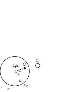
Figure 1: Illustrative representation of an ion of charge $Q$ near a colloidal particle and the induced image, $Q^{\prime}$, and counterimage, $\lambda(u)$, charges.

Although Eqs. 3 and 4 are exact, they are not very useful for Monte-Carlo or molecular dynamics simulations — the integral in Eq. 3 must be done numerically for each new configuration of ions, making simulations very slow. However, we can consider a simplifying approximation. We note that the dielectric constant of a colloidal particle is much smaller than the dielectric constant of the surrounding medium. Thus, to leading order in $\epsilon_{c}/\epsilon_{w}$ we can take $\gamma\approx 1$. In this case the counterimage charge is uniformly distributed, $\bar{\lambda}(u)=-Q^{\prime}/r^{\prime}_{i}$, and the integral in Eq. 3 can be performed exactly, yielding the counterimage potential at an arbitrary position ${\bf r}$,

$$\bar{\psi}_{ci}({\bf r};{\bf r}_{i})=\dfrac{\alpha q}{\epsilon_{w}a}\log\left(\frac{rr_{i}-{\bf r}\cdot{\bf r_{i}}}{a^{2}-{\bf r}\cdot{\bf r_{i}}+\sqrt{a^{4}-2a^{2}({\bf r}\cdot{\bf r_{i}})+r^{2}r_{i}^{2}}}\right)\ ,$$ (5)

where the over-bar is used to denote the uniform line-charge approximation. The ion-counterimage interaction potential also reduces to a simple equation,

$$\bar{\psi}_{ci}^{self}({\bf r}_{i})=\dfrac{\alpha q}{\epsilon_{w}a}\log\left(1-\frac{a^{2}}{r_{i}^{2}}\right)\ .$$ (6)

III Monte Carlo Simulations

The simulations are performed inside a spherical Wigner-Seitz (WS) cell of radius $R$ with a colloidal particle of charge $-Zq$ placed at the center. The cell also contains $N=Z/\alpha$ $\alpha$-valent counterions each of diameter $d$. The electrostatic potential produced at position ${\bf r}$ by an ion located at ${\bf r}_{i}$ is

$$\phi({\bf r};{\bf r}_{i})=\dfrac{\alpha q}{\epsilon_{w}|{\bf r}-{\bf r}_{i}|}+\dfrac{\gamma\alpha qa}{\epsilon_{w}r_{i}|{\bf r}-\frac{a^{2}}{r_{i}^{2}}{\bf r}_{i}|}+\gamma\bar{\psi}_{ci}({\bf r};{\bf r}_{i})\ ,$$ (7)

where the first term is the electrostatic potential produced by the ion and the second and the third terms are the potentials produced by the image and the counterimage charges, respectively. The first two terms of Eq. 7 are exact. In the third term we have used the condition of charge neutrality to correct the ion-counterimage interaction from Eq. 5 by including a prefactor $\gamma$ in front of $\bar{\psi}_{ci}({\bf r};{\bf r}_{i})$. This, then, is the Green function for the present geometry. The interaction potential between two ions $i$ and $j$ is $\alpha q\phi({\bf r}_{i};{\bf r}_{j})$. The work required to bring all the ions from infinity to their respective positions inside the cell is,

$$U=\sum_{i=1}^{N}-\dfrac{Z\alpha q^{2}}{\epsilon_{w}r_{i}}+\sum_{i=1}^{N}U_{i}^{self}+\sum_{i=1}^{N-1}\sum_{j=i+1}^{N}\alpha q\phi({\bf r}_{i};{\bf r}_{j})\ ,$$ (8)

$$U_{i}^{self}=\dfrac{\gamma\alpha^{2}q^{2}a}{2\epsilon_{w}(r_{i}^{2}-a^{2})}+\dfrac{\alpha q\gamma\bar{\psi}_{ci}^{self}({\bf r}_{i})}{2}\ ,$$ (9)

where $U_{i}^{self}$ is the interaction energy of the ion $i$ with its image and counterimage charges.

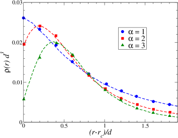
Figure 2: The dashed lines represent the density profiles obtained using the present method and the symbols represent the profiles obtained by Messina Messina (2002). The parameters of the simulations are: $\epsilon_{w}=80$, $\epsilon_{c}=2$, $d=3.57$Å, $a=7.5d$, $R=40d$, $Z=60$, and $r_{c}=a+d/2$ is the contact distance.

We use the Eq. 8 in a typical Metropolis algorithm Allen and Tildesley (1987), with $10^{5}$ MC steps for equilibration and $10^{4}$ steps for production. We obtain the ionic density profiles dividing the WS cell in volumetric bins and counting the average number of particles in each bin for all uncorrelated configurations. In Fig. 2 the profiles are compared with the ones obtained by Messina Messina (2002). The agreement between the two simulations is excellent, with a huge gain in computational time. To take into account the correct boundary conditions, Messina calculated the inter-ionic interaction potential as an infinite series in Legendre polynomials. This method is extremely slow, since one needs to calculate hundreds of terms of the infinite series for each new configuration in order to obtain a good convergence. To compare the time of processing, we perform the simulation of Messina for parameters described in Fig. 2 with trivalent ions. Even for a very small number of counterions — twenty counterions — used by Messina, expansion in Legendre polynomials is $\approx 458\times$ slower than the method presented in the current paper. To speed up the simulations Messina tabulated the counterion-counterion interaction potential. Nevertheless, his approach remains at least one order of magnitude slower than our Green function method, and is significantly more difficult to extend to larger system sizes.

The approximation of the counterimage charge by a uniform line-charge density, should work very well for colloids of low dielectric constants, which are of most practical interest. However, it is interesting to examine up to what value of $\epsilon_{c}$ does this approximation remains accurate. Using the exact numerical evaluation of the integral in Eq. 3, and the hypergeometric representation of the counterimage-ion interaction potential Eq. 4, we have performed the simulations for different values of $\epsilon_{c}$ using the exact numerically calculated interaction potential and compared the counterion density profiles with the ones obtained in simulations with the approximate interaction potentials, Eqs. 5 and 6. In Fig. 3 we show the results of these simulations. We see that the approximation works very well up to $\epsilon_{c}\approx 20$, which are in the range of most practical interest.

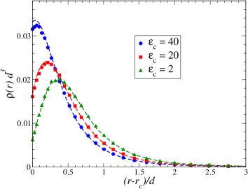
Figure 3: Density profiles for various $\epsilon_{c}$. The symbols represent the density profiles obtained using the exact counterimage line-charge distribution, while the dashed lines are calculated using the approximate uniform counterimage line-charge distribution, Eqs. 5 and 6. The parameters of the simulations are the same as in Fig. 2, for $\alpha=3$.

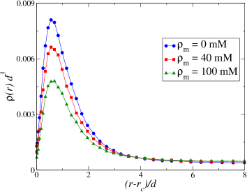
Figure 4: Density profiles of trivalent counterions for various concentrations of 1:1 electrolyte. The parameters of the simulations are the same as in Fig. 2 for $R=25d$, $\alpha=1$ and $Z=40$. The 3:1 concentration is $20$ mM.

The simulations using the method developed in the present work are so quick that it is easy to study systems which contain mixtures of multivalent and monovalent electrolytes. We next consider a WS cell that contain 3:1 electrolyte at concentration $\rho_{t}$ and 1:1 electrolyte at concentration $\rho_{m}$. The number of trivalent counterions inside the system is $N_{t}=\rho_{t}\frac{4\pi}{3}(R^{3}-a^{3})$, the number of monovalent counterions is $N_{m}=\rho_{m}\frac{4\pi}{3}(R^{3}-a^{3})$ and the number of monovalent coions is $N_{-}=3N_{t}+N_{m}$. In Fig. 4, the density profiles of 3:1 salt cations are presented for various concentration of 1:1 salt. As expected, with increase of the monovalent salt concentration, more trivalent cations prefer to be solvated in the bulk of suspension, where their electrostatic self-energy is screened most effectively by the other ions Pianegonda, Barbosa, and Levin (2005); dos Santos, Diehl, and Levin (2010).

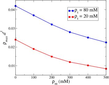
Figure 5: Maximum density of trivalent salt counterions as function of concentration of 1:1 electrolyte. The parameters of the simulations are: $\epsilon_{w}=80$, $\epsilon_{c}=0$, $d=4$Å, $a=30$Å, $R=70$Å and $Z=90$.

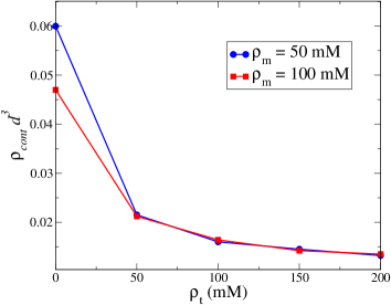
Figure 6: The density at contact of monovalent counterions for varying concentrations of 3:1 electrolyte. The parameters of the simulations are the same as in Fig. 5.

The charge-image repulsion results in density profiles of trivalent ions which have a characteristic maximum near the colloidal surface. In Fig. 5, we examine the effects of 3:1 and 1:1 electrolyte on the maximum density of trivalent counterions near the colloidal surface. Again we see that increasing the concentration of 1:1 electrolyte diminishes the counterion condensation — resulting in a smaller counterion density in the vicinity of the colloidal surface. More surprising, perhaps, is the behavior of the contact density of the monovalent counterions, Fig. 6. We see that at small concentrations of 3:1 electrolyte the contact density varies significantly with the concentration of 1:1 electrolyte. This dependence, however, rapidly saturates, so that for $50$ mM of 3:1 electrolyte, we no longer see any variation of the contact density with the concentration of 1:1 salt. The Fig. 6 shows that with increasing 3:1 concentration the condensed monovalent counterions are rapidly replaced by the trivalent ones.

IV Conclusions

We have presented a very efficient method for simulating colloidal suspension composed of lyophobic colloidal particles of low dielectric constant. The method relies on the exact calculation of the Green function for the spherical geometry. The results are in excellent agreement with the earlier simulations of Messina Messina (2002) — who used expansion in Legendre polynomials to account for the dielectric discontinuity at the colloidal surface — with a huge gain in the computation time. At the moment, we have only implemented the simulation inside a WS cell geometry. In the future, an effort should be made to extend the theory to take into account periodic boundary conditions through the use of Ewald summation.

This work was partially supported by the CNPq, Fapergs, INCT-FCx, and by the US-AFOSR under the grant FA9550-09-1-0283.

References

- Miraballes-Martinez and Forcada (2000) I. Miraballes-Martinez and J. Forcada, J. Polym. Sci. Pol. Chem. 38, 4230 (2000).
- Miraballes-Martinez et al. (2001) I. Miraballes-Martinez, A. Martin-Molina, F. Galisteo-Gonzalez, and J. Forcada, J. Polym. Sci. Pol. Chem. 39, 2929 (2001).
- Levin (2002) Y. Levin, Rep. Prog. Phys. 65, 1577 (2002).
- Lopez-Leon et al. (2003) T. Lopez-Leon, A. B. Jodar-Reyes, D. Bastos-Gonzalez, and J. L. Ortega-Vinuesa, J. Phys. Chem. B 107, 5696 (2003).
- Lopez-Leon et al. (2008) T. Lopez-Leon, M. J. Santander-Ortega, J. L. Ortega-Vinuesa, and D. Bastos-Gonzalez, J. Phys. Chem. C 112, 16060 (2008).
- Peula-Garcia, Ortega-Vinuesa, and Bastos-Gonzalez (2010) J. M. Peula-Garcia, J. L. Ortega-Vinuesa, and D. Bastos-Gonzalez, J. Phys. Chem. C 114, 11133 (2010).
- dos Santos and Levin (2011) A. P. dos Santos and Y. Levin, Phys. Rev. Lett. 106, 167801 (2011).
- Rouzina and Bloomfield (1996) I. Rouzina and V. Bloomfield, J. Chem. Phys. 100, 9977 (1996).
- Linse and Lobaskin (1999) P. Linse and V. Lobaskin, Phys. Rev. Lett. 83, 4208 (1999).
- Wu et al. (1999) J. Z. Wu, D. Bratko, H. W. Blanch, and J. M. Prausnitz, J. Chem. Phys. 111, 7084 (1999).
- Gelbart et al. (2000) W. M. Gelbart, R. F. Bruinsma, P. A. Pincus, and V. A. Parsegian, Phys. Today 53, 38 (2000).
- Solis and de la Cruz (2001) F. J. Solis and M. O. de la Cruz, Phys. Today 54, 71 (2001).
- Lozada-Cassou, Saavedra-Barrera, and Henderson (1982) M. Lozada-Cassou, R. Saavedra-Barrera, and D. Henderson, J. Chem. Phys. 77, 5150 (1982).
- Pianegonda, Barbosa, and Levin (2005) S. Pianegonda, M. Barbosa, and Y. Levin, Europhys. Lett. 71, 831 (2005).
- Diehl and Levin (2006) A. Diehl and Y. Levin, J. Chem. Phys. 125, 054902 (2006).
- Diehl and Levin (2008) A. Diehl and Y. Levin, J. Chem. Phys. 129, 124506 (2008).
- Guerrero-Garcia, Gonzalez-Tovar, and de la Cruz (2010) G. I. Guerrero-Garcia, E. Gonzalez-Tovar, and M. O. de la Cruz, Soft Matter 6, 2056 (2010).
- dos Santos, Diehl, and Levin (2010) A. P. dos Santos, A. Diehl, and Y. Levin, J. Chem. Phys. 132, 104105 (2010).
- Quesada-Pérez, Callejas-Fernández, and Hidalgo-Álvarez (2002) M. Quesada-Pérez, J. Callejas-Fernández, and R. Hidalgo-Álvarez, Adv. Colloid Inter. Sci. 95, 295 (2002).
- Fernandez-Nieves et al. (2005) A. Fernandez-Nieves, A. Fernandez-Barbero, F. J. de las Nieves, and B. Vincent, J. Chem. Phys. 123, 054905 (2005).
- Linse (1986) P. Linse, J. Phys. Chem. 90, 6821 (1986).
- J. D. Jackson (1999) J. D. Jackson, Classical Electrodynamics (Wiley, New York, 1999).
- Lindell (1992) I. V. Lindell, Radio Sci. 27, 1 (1992).
- Norris (1995) W. T. Norris, IEE P-Sci. Meas. Tech. 142, 142 (1995).
- Reed, Lanning, and Madden (2007) S. K. Reed, O. J. Lanning, and P. A. Madden, J. Chem. Phys. 126, 084704 (2007).
- Reed, Madden, and Papadopoulos (2008) S. K. Reed, P. A. Madden, and A. Papadopoulos, J. Chem. Phys. 128, 124701 (2008).
- Loth, Skinner, and Shklovskii (2010) M. S. Loth, B. Skinner, and B. Shklovskii, Phys. Rev. E 82, 016107 (2010).
- Outhwaite, Lamperski, and Bhuiyan (2011) C. W. Outhwaite, S. Lamperski, and L. B. Bhuiyan, Mol. Phys. 109, 21 (2011).
- Messina (2004) R. Messina, Phys. Rev. E 70, 051802 (2004).
- Messina (2006) R. Messina, Phys. Rev. E 74, 049906 (2006).
- Seijo et al. (2009) M. Seijo, M. Pohl, S. Ulrich, and S. Stoll, J. Chem. Phys. 131, 174704 (2009).
- Messina (2002) R. Messina, J. Chem. Phys. 117, 11062 (2002).
- Allen and Tildesley (1987) M. P. Allen and D. J. Tildesley, Computer Simulations of Liquids (Oxford: Oxford University Press, 1987).