An alternative method for simulating particle suspensions using lattice Boltzmann
Abstract
In this study, we propose an alternative way to simulate particle suspensions using the lattice Boltzmann method. The main idea is to impose the non-slip boundary condition in the lattice sites located on the particle boundaries. The focus on the lattice sites, instead of the links between them, as done in the more used methods, represents a great simplification in the algorithm. A fully description of the method will be presented, in addition to simulations comparing the proposed method with other methods and, also, with experimental results.
Keywords: Lattice Boltzmann method, Particulate flow, Particle-fluid interactions
1 Introduction
Particulate flows are found in many industrial processes
[1, 2, 3, 4],
and have been subjected to considerable scientific investigation.
Recently, computer simulations have become an effective tool in these studies and
several methods have been applied, such as finite element method [5],
Lagrange-multipliers [2, 3], direct forcing
method [6], lattice Boltzmann methods
[1, 4, 7, 8, 9, 10, 11, 12, 13, 14, 15, 16],
solving the Stokes equation near
the particles (Physalis) [17] and combining two or more methods
[14, 18, 19].
In this study, we propose an alternative way to simulate suspensions
using the lattice Boltzmann method. The main idea is to impose the
non-slip boundary condition in the lattice sites representing the
particle boundaries. The focus on lattice sites, instead of the link between
them, as done in the more used methods [11], represents
a great simplification in the algorithm. Similar approaches, focusing
on the lattice sites were already tried [1], although without popularity
due, probably, to difficulties several in the implementation.
Its important to mention that the simplifications we propose
can reduce the accuracy in describing the details of the flow near
the particles, and these details can or cannot be important, depending
on the problem one wants to simulate.
In the simulations we have done until now, in despite of the
simplifications, the results we obtain are similar to the results
obtained by other methods (see section 3).
2 The model
In this section we introduce the lattice Boltzmann method and present the model describing the particle-fluid interaction. Interactions among particles and between a particle and a solid surface will also be discussed in this section.
2.1 The lattice Boltzmann model
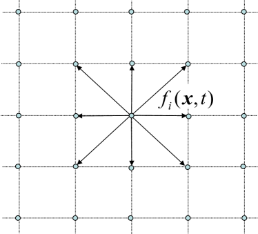
The lattice-Boltzmann method (LBM) is based on the discretization of the Boltzmann’s mesoscopic equation[20, 21, 22], usually with the BGK approach for the collision operator (for a comprehensive review see [23]). In the LBM scale, the system is described using a single particle distribution function, , representing the number of particles with velocity at the site and time , where . The particles are restricted to a discrete lattice, in a manner that each group of particles can move only in a finite number of directions and with a limited number of velocities (see Fig. 1). Therefore, physical and velocity space are discretized.
The local macroscopic properties such as total mass (the particle mass, m, is assumed unitary), , and total momentum, , can be obtained from the distribution function in the following way:
| (1) |
| (2) |
The Lattice Boltzmann equation, that is, the discrete version of the Boltzmann equation with the BGK collision, operator is written
| (3) |
where, is the time step and is a polynomial approximation of the Maxwell-Boltzmann equilibrium distribution [24, 20, 21, 22], a function of the local variables and . It can be shown, through a Chapman-Enskog analysis, that this system macroscopically will evolve according to the Navier-Stokes equations with a kinematic viscosity given by
| (4) |
where is the sound velocity, a constant depending on the set of velocities .
2.2 Particle-fluid interaction
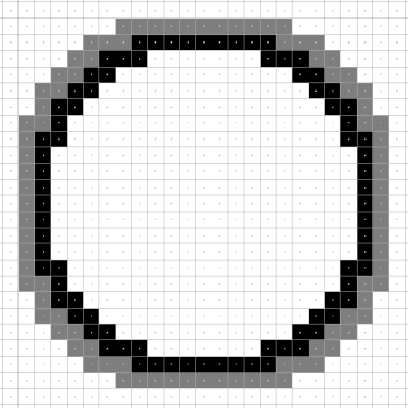
The basic idea of the method is that the fluid in contact with a solid surface must acquire the velocity of this surface, considering the non-slip condition. Keeping this in mind, a set of boundary sites can be used to describe the particle. This approach is similar to the one presented in [7] and [11], although we focus in the lattice sites and not in the links between them. We denote boundary sites (BS) the particle sites in contact with fluid, and internal sites (IS) the particle sites in contact with the boundary sites (see Fig.2). The particle’s boundary is regarded to be halfway between the IS and the BS sites.
A particle will be represented by its central position , a radius , a mass and a moment of inertia . Its velocity will be denoted , and the angular velocity . Only spherical particles will be considered.
The presence of a particle will be represented only by its effects on the fluid in contact with the particle, altering the dynamics of the sites BS and IS. The position of these sites will be denoted by and , respectively, and its integer counterpart (or the nearest integer of each component of the vectors) by and , respectively. Velocities and densities in the sites and will be denoted , and , . We emphasize that all sites will be updated by the usual collision/propagation steps, but the IS and BS sites, in addition to these steps, will be submitted to a set of substeps included between the collision and the propagation steps. These substeps are presented in the sequence.
-
•
Particle-fluid momentum transfer
This substep is executed only in the BS sites. As was previously mentioned, the velocity in the BS sites must acquire the particle’s velocity. This velocity, considering the angular velocity, is
| (5) |
To impose this velocity in the fluid, that is in lattice sites, the equilibrium distribution is employed, setting .
Naming the linear momentum of a BS site, we compute
| (6) |
and
| (7) |
where represents the change in the angular momentum caused by the change in the linear momentum .
Finishing this step we have the total momentum exchanged, and :
| (8) |
| (9) |
-
•
Particle’s acceleration
This substep accounts for the change in particles velocity caused by fluid. According to the Newton’s third law of motion, we simply compute
| (10) |
| (11) |
| (12) |
-
•
Updating of particle’s position
Due to the spherical symmetry it is not necessary to take into account the rotation of the particles. The position is updated by doing:
| (13) |
The positions of boundary and internal sites, also, must be updated:
| (14) |
| (15) |
Clearly, this procedure includes errors of order (), more precise procedures could be employed. Nevertheless, there is a lot of imprecision in describing the shape of the particle, therefore it is not necessary to be so precise in updating particle’s position.
-
•
Velocity of the internal sites
To impose this velocity the equilibrium distribution is employed again,
setting
.
Some comments are necessary to clarity the physics behind these sub-steps.
Consider a particule that is found with a velocity different of the fluid
velocity around it, in the beginning of the particle-fluid interaction step.
This situation never occurs in the continuum but this is possible in discrete models
due to the discretization of time. Particle and fluid must then exchange linear and
angular momentum until the fluid around the particle acquires the velocity of
the particle surface. In this process the particle velocity also changes due
to the fluid reaction on the particle and in accordance with Newton’s third law
of motion. Action and reaction happen simultaneously in the physical process,
but in the discrete case this occurs in steps 1 and 2. In the
first step the particle transfers linear and angular momentum to the fluid.
In consequence the fluid in contact with the particle surface particle accelerates
until have acquired the same particle velocity. As it was earlier mentioned two
hypotheses are used for this step: non-slipping on the particle surface
and the hypotheses that the fluid-particle equilibration takes a time interval
smaller than the time step used in the simulation.
This enables the use of an equilibrium distribution to impose the velocities.
With the fluid velocity altered, we then calculate the change in the linear and
angular momentum of the fluid due to this acceleration. These variations must
be the same as the corresponding changes for the particle, in accordance with
the Newton’s third law. We then proceed to step 2 and recalculate the
particle velocity. The velocity to be imposed in sites IS is also calculated in
accordance with the new particle velocity.
In a third step, the position of the particle and sites IS and BS are changed. The spherical symmetry of the particles eases this step since only the translation velocities are taken into account in the calculation of the new positions. It must be stressed that although sites BS belong to the fluid phase, they have their position changed in accordance with the particle velocity. Indeed, these sites are in the particle boundary and must follow its displacement. In other words the displacement of the boundary sites is independent of the fluid particles that are occupying these sites, in a given instant.
Finally, in a fourth step, we impose the velocity to the sites IS. This step is important because during the propagation step the information in these sites is transferred to the adjacent sites BS. Therefore, the sites BS will have their velocity composed by the particle and fluid velocities and will define a new change of momentum in the following time step.
2.3 Interaction between particles
Especially in simulations involving a great number of particles,
as the simulation presented in subsection 3.4, the interaction
between particles must carefully be addressed. There are many
techniques to treat these interactions, possibly the most popular
approach is to introduce a
repulsive force between particles when the gap
between becomes smaller than a given threshold[14]. We chose another approach
in this work, treating the collisions as occurring between completely
rigid particles (hard-core collisions). In this way it is not necessary to set
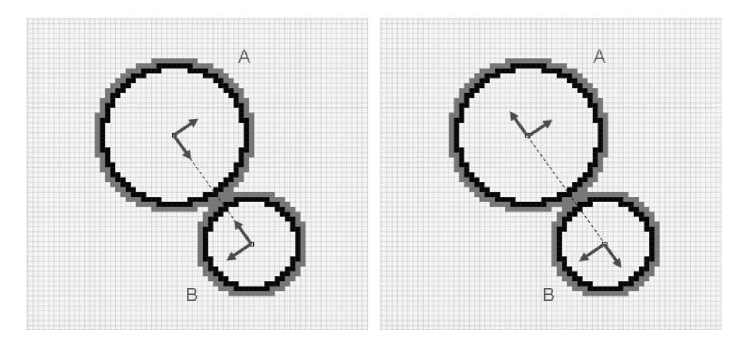
the parameters of repulsive forces. We simply impose (see Fig.3)
| (16) |
| (17) |
| (18) |
| (19) |
where all velocities are represented in the center of mass reference frame.
This imposition must be done before updating particles’ positions, that is, it can
be considered as part of the particle’s acceleration substep.
It’s necessary to underline that the way we chose to
introduce the particle-particle interaction is not new, nor regarded as part of
the method. Moreover, this choice was done considering solely
the easeness in the implementation. In accordance with the Reynolds number,
volume fraction of the particles and the involved force, more elaborated
techniques, employing lubrication[8] or spring forces[25]
may reveal to be necessary.
3 Validation
Four cases are presented in order to validate the model. The first case simulated was the flow around a massive two-dimensional particle. The particle’s mass was chosen in such way that it doesn’t move, therefore it’s possible to compare the flow around the two dimensional particle and the flow around a solid cylinder, simulated using bounce-back. The drag coefficient for a massive particle was also computed considering several Reynolds number and compared with drag coefficients obtained by other methods. The second case simulated was the flow of a neutrally buoyant two-dimensional particle in a shear flow, the results are compared with the results presented by Feng and Michaelides[14]. A simulation of a sphere settling in a closed box was done in order to validate the model in a three-dimensional simulation. The results obtained was compared with the ones presented by ten Cate et al.[26]. Finally, it was simulated the sedimentation of 504 two-dimensional particles in an enclosure.
3.1 Flow around a massive two dimensional particle
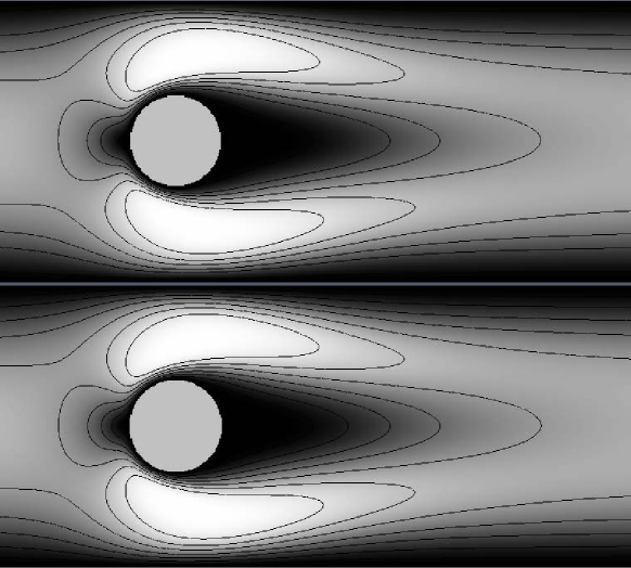
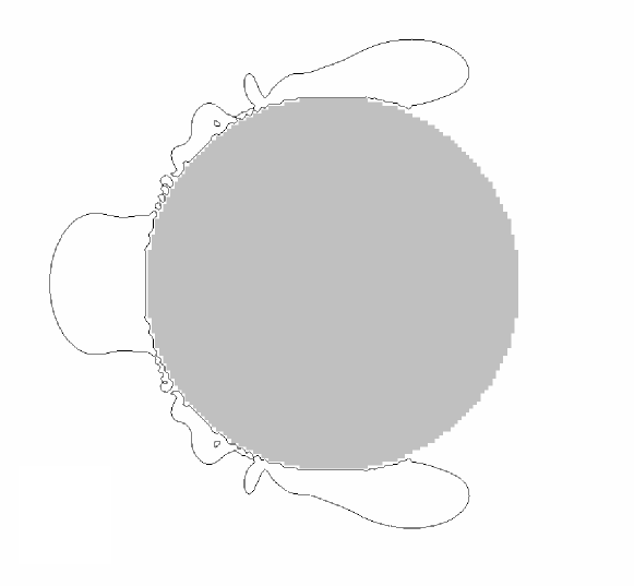
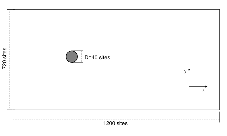
The first geometry used to simulate the flow around a massive particle is depicted in Fig. 4. The simulations of a flow around a solid cylinder was carried out using bounce-back boundary conditions and the simulation of flow around a massive particle was done using the method proposed in this work, that is, using the equilibrium distribution to impose the velocities in the boundaries of the particle. The results of both simulations are presented in Fig. 5. To emphasize the deviations we plot in Fig. 6 the magnitude of the difference between the velocities. In the enclosed regions of Fig. 6 the deviations are of order (the velocities in the simulations varying from zero to ). Is important to notice that, in despite of deviations that can appear near the solid surface as result of applying different boundary conditions, the overall flow behavior is the same. Off course, depending on the applications ones intends to focus, these differences must be taken into account.
.
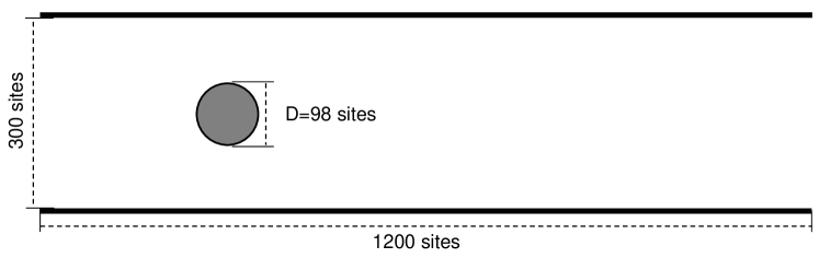
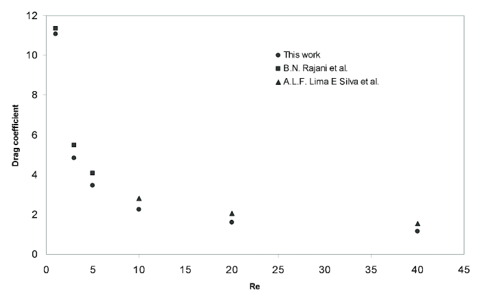
Simulations to obtain drag coefficients were also carried out in the geometry presented in Fig. 7. Velocities varying from 0.00417 to 0.1667 in the x direction were imposed at the boundaries (left, right, top and bottom), resulting in the Reynolds number varying from to . The results obtained are shown in Fig. 8, beside the results published by Rajani et al.[27] and Silva et al. [28]. Although the drag coefficients computed in this work were systematically lower than the results obtained by other methods, the importance of these errors is dependent on what we want to describe in a given problem,as it can be seen in the simulations presented in the sequence.
3.2 Neutrally buoyant two dimensional particle in a shear flow
The motion of a neutrally buoyant two-dimensional particle moving in viscous fluid was already simulated using LBM [29],[30],[14] as well as using finite element method [5] , and was chosen as one of the validations of the present model. The geometry of the problem is described in Fig. 9, where and are the velocities imposed. Periodic boundary conditions are imposed in the left and right boundaries. The relaxation time was set , which implies a kinematic viscosity , in lattice units.
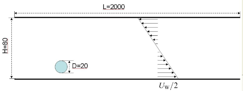
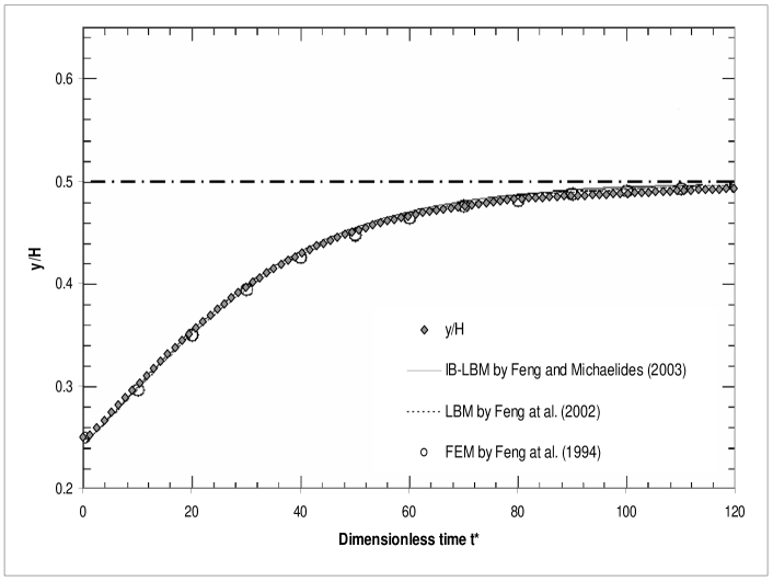
The parameters chosen are the same used in Feng & Michaelides paper[14], in order to ease the comparison. The velocity equals , therefore, the shear rate for the flow is , and a dimensionless time, , is defined , where is the particle radius. Fig. 10, shows the migration of the particle, initially at the position , toward the center. The agreement between the results using the proposed model and the previous models are quite good.
3.3 A sphere settling in a closed box
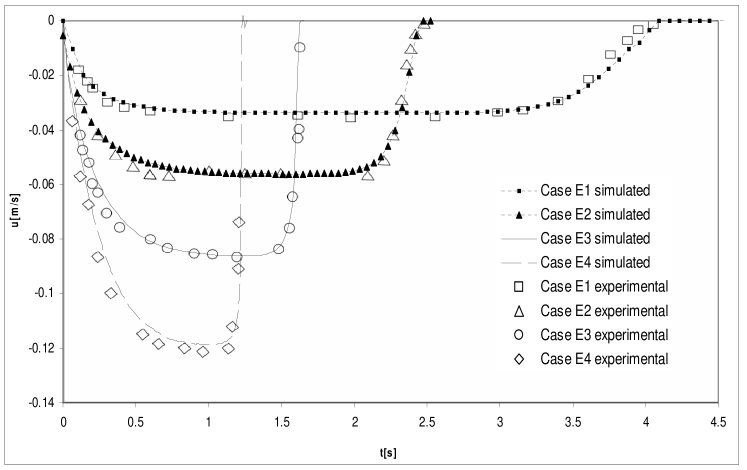
In this subsection the trajectory and velocity of a sphere settling in a closed box is simulated using the model here prosed and compared with experimental results obtained by Cate et al. [26].
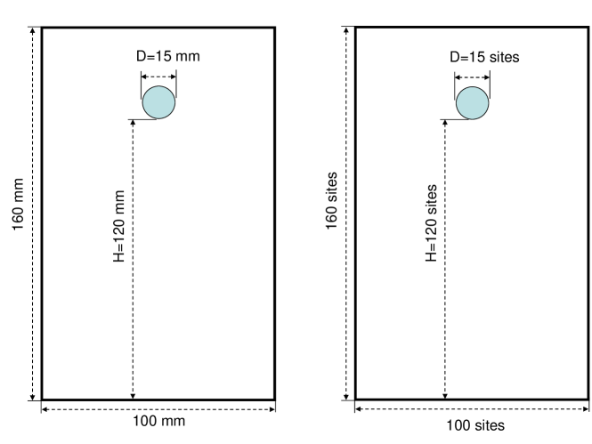
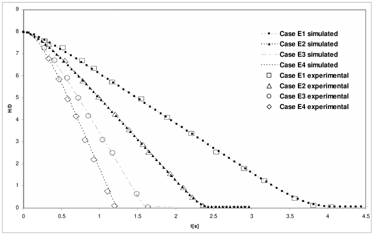
The settling sphere has a diameter of and density . The container dimensions are depthwidthheight (see Fig. 11). Four cases were simulated considering the different densities and viscosities of the fluid in which the sphere will settle, corresponding to a Reynolds number varying from to . The fluid characteristics and the parameters used in the simulations are shown in Table 1.
| Case E1 | 970 | 373 | 0.9 | 0.347 |
| Case E2 | 965 | 212 | 0.9 | 0.607 |
| Case E3 | 962 | 113 | 0.8 | 0.851 |
| Case E4 | 960 | 58 | 0.9 | 2.207 |
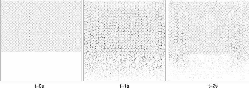
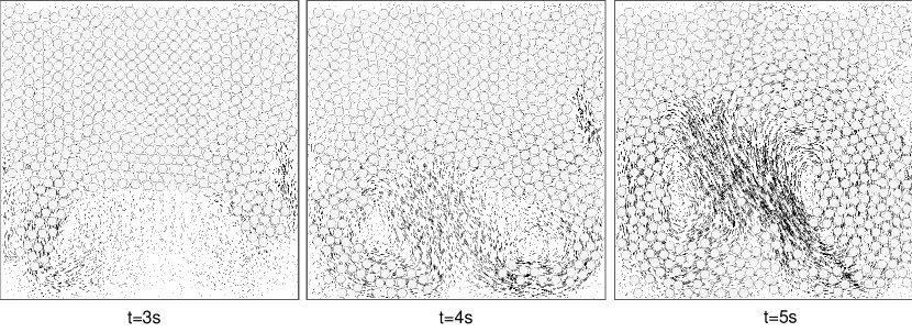
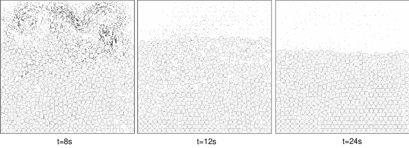
3.4 504 particles settling in a closed box
The problem of a large number of particles settling in a closed 2D box was already simulated by other methods [2], [14]. All the parameters were chosen in order to compare with the previous works. That is, 504 circular particles with diameter settling in box having width and height. The fluid and particle densities are and , respectively, and the fluid kinematic viscosity is . Representing the box by sites and using a relaxation time we will have a time step of . The process of sedimentation simulated from the initial state to is presented in Fig. 14, Fig. 15 and Fig. 16. The figures show the development of a Rayleigh–Taylor instability and are, qualitatively, in agreement with the previous works. The differences between the three simulations (the one presented here and the simulations of refs. [2] and [14]) are, possibly, a result of the differences in treating the collisions between particles and differences arising from compressibility effects that are present in the lattice Boltzmann methods.
4 Conclusion
In this study an alternative and simpler way to simulate particle-fluid interactions is proposed. The lattice Boltzmann method is employed to simulate the fluid flow and the particles are simulated using the Newton’s law. The coupling is made applying the equilibrium distribution function to assure the non-slip condition near the solid surfaces. Several simulations are presented showing that the method can simulate particle-fluid interactions with a precision comparable with other methods.
References
References
- [1] O. Behrend, “Solid–fluid boundaries in particle suspension simulations via the lattice boltzmann method,” Physical Review E 52, pp. 1164–1175, 1995.
- [2] R. Glowinski, T. W. Pan, T. I. Hesla, and D. D. Joseph, “A distributed lagrange multiplier/fictitious domain method for particulate flows,” International Journal of Multiphase Flow 25, pp. 755–794, 1999.
- [3] N. Patankar, P. Singh, D. Joseph, R. Glowinski, and T. W. Pan, “A new formulation of the distributed lagrange multiplier/ fictitious domain method for particulate flows,” International Journal of Multiphase Flow 26, pp. 1509–1524, 2000.
- [4] E.-J. Ding and C. K. Aidun, “Extension of the lattice-boltzmann method for direct simulation of suspended particles near contact,” Journal of Statistical Physics 112, pp. 685–708, August 2003.
- [5] J. Feng, H. H. Hu, and D. D. Joseph, “Direct simulation of initial-value problems for the motion of solid bodies in a newtonian fluid .2. couette and poiseuille flows,” Journal of Fluid Mechanics 277, pp. 271–301, 1994.
- [6] Z. Yu and X. Shao, “A direct-forcing fictitious domain method for particulate flows,” Journal of Computational Physics 227, pp. 292–314, 2007.
- [7] A. Ladd, “Numerical simulation of particulate suspension via a discretized boltzmann-equation .1. theoretical foundation,” Journal of Fluid Mechanics 271, pp. 285–309, 1994.
- [8] A. Ladd, “Numerical simulation of particulate suspension via a discretized boltzmann-equation .2. numerical results,” Journal of Fluid Mechanics 271, pp. 311–339, 1994.
- [9] C. Aidun and Y. Lu, “Lattice boltzmann simulation of solid particles suspended in a fluid,” Journal of Statistical Physics 81, pp. 49–59, 1995.
- [10] C. Aidun, Y. Lu, and E.-J. Ding, “Direct analysis of particulate suspensions with inertia using the discrete boltzmann equation,” Journal of Fluid Mechanics 373, pp. 287–311, 1998.
- [11] A. J. C. Ladd and R. Verberg, “Lattice-boltzmann simulations of particle-fluid suspensions,” Journal of Statistical Physics 104, pp. 1191–1251, September 2001.
- [12] B. Chopard and S. Marconi, “Lattice boltzmann solid particles in a lattice boltzmann fluid,” Journal of Statistical Physics 107, pp. 23–37, April 2002.
- [13] N.-Q. Nguyen and A. J. C. Ladd, “Lubrication corrections for lattice-boltzmann simulations of particle suspensions,” Physical Review E 66, p. 046708, 2002.
- [14] Z.-G. Feng and E. E. Michaelides, “The immersed boundary-lattice boltzmann method for solving fluid -particles interaction problems,” Journal of Computational Physics 195, pp. 602–628, 2004.
- [15] N.-Q. Nguyen and A. J. C. Ladd, “Sedimentation of hard-sphere suspensions at low reynolds number,” Journal of Fluid Mechanics 525, pp. 73 –104, 2005.
- [16] J. Kromkamp, D. van den Ende, D. Kandhai, R. van der Sman, and R. Boom, “Lattice boltzmann simulation of 2d and 3d non-brownian suspensions in couette flow,” Chemical Engineering Science 61, pp. 858–873, 2006.
- [17] Z. Zhang and A. Prosperetti, “A second-order method for three-dimensional particle simulation,” Journal of Computational Physics 210, pp. 292–324, 2005.
- [18] Z.-G. Feng and E. E. Michaelides, “Proteus: a direct forcing method in the simulations of particulate flows,” Journal of Computational Physics 202, pp. 20–51, 2005.
- [19] Z. Wang, J. Fan, and K. Luo, “Combined multi-direct forcing and immersed boundary method for simulating flows with moving particles,” International Journal of Multiphase Flow 34(3), pp. 283–302, 2008.
- [20] X. He and L. Luo, “A priori derivation of the lattice boltzmann equation,” Physical Review E 55(6), pp. R6333–R6336, 1997.
- [21] X. Shan, X.-F. Yuan, and H. Chen, “Kinetic theory representation of hydrodynamics: a way beyond navier-stokes equation,” Journal of Fluid Mechanics 550, pp. 413–441, 2006.
- [22] P. C. Philippi, L. A. Hegele, L. O. E. dos Santos, and R. Surmas, “From the continuous to the lattice boltzmann equation: The discretization problem and thermal models,” Physical Review E 73(5), p. 056702, 2006.
- [23] S. Succi, The Lattice Boltzmann Equation for Fluid Dynamics and Beyond, Oxford University Press, 2001.
- [24] T. Abe, “Derivation of the lattice boltzmann method by means of the discrete ordinate method for the boltzmann equation,” Journal of Computational Physics 131(1), pp. 241–246, 1997.
- [25] K. Höfler and S. Schwarzer, “Navier-stokes simulation with constraint forces: Finite-difference method for particle-laden flows and complex geometries,” Physical Review E 61(6), pp. 7146–7160, 2000.
- [26] A. ten Cate, C. H. Nieuwstad, J. J. Derksen, and H. E. A. V. den Akker, “Particle imaging velocimetry experiments and lattice-boltzmann simulations on a single sphere settling under gravity,” Physics of Fluids 14, pp. 4012–4025, November 2002.
- [27] B. Rajani, A. Kandasamy, and S. Majumdar, “Numerical simulation of laminar flow past a circular cylinder,” Applied Mathematical Modelling 33, pp. 1228 –1247, 2009.
- [28] A. L. E. Silva, A. Silveira-Neto, and J. Damasceno, “Numerical simulation of two-dimensional flows over a circular cylinder using the immersed boundary method,” Journal of Computational Physics 189, pp. 351 –370, 2003.
- [29] Z.-G. Feng and E. E. Michaelides, “Hydrodynamic force on spheres in cylindrical and prismatic enclosures,” International Journal of Multiphase Flow 28, pp. 479–496, 2002.
- [30] Z.-G. Feng and E. E. Michaelides, “Interparticle forces and lift on a particle attached to a solid boundary in suspension flow,” Physics of Fluids 14, pp. 49–60, January 2002.