Shock Dynamics in Layered Periodic Media

Abstract

Solutions of constant-coefficient nonlinear hyperbolic PDEs generically develop shocks, even if the initial data is smooth. Solutions of hyperbolic PDEs with variable coefficients can behave very differently. We investigate formation and stability of shock waves in a one-dimensional periodic layered medium by computational study of time-reversibility and entropy evolution. We find that periodic layered media tend to inhibit shock formation. For small initial conditions and large impedance variation, no shock formation is detected even after times much greater than the time of shock formation in a homogeneous medium. Furthermore, weak shocks are observed to be dynamically unstable in the sense that they do not lead to significant long-term entropy decay. We propose a characteristic condition for admissibility of shocks in heterogeneous media that generalizes the classical Lax entropy condition and accurately predicts the formation or absence of shocks in these media.

1 Introduction

Consider one-dimensional nonlinear wave propagation in a spatially heterogeneous medium, described by the first order hyperbolic system

$$\epsilon_{t}(x,t)-u_{x}(x,t) =0$$ (1a)

$$\rho(x)u(x,t)_{t}-\sigma(\epsilon(x,t),x)_{x} =0.$$ (1b)

This system is a rather generic description of nonlinear waves in a Lagrangian frame, and arises in a variety of contexts including elasticity, optics, and gas dynamics. In the case of elasticity, $\epsilon,\sigma,\rho$, and $u$ are the strain, stress, density, and velocity, respectively.

All the results presented in this work involve a simple periodic medium composed of alternating homogeneous layers of materials A and B:

$$(\rho(x),K(x)) =\left\{\begin{array}[]{ll}(\rho_{A},K_{A})&\text{if }j<x<(j+1/2)\mbox{ for some integer j},\\ (\rho_{B},K_{B})&\mbox{otherwise.}\end{array}\right.$$ (4)

with nonlinear stress-strain relation

$$\sigma(\epsilon,x)=\exp(K(x)\epsilon)-1,$$ (5)

Further computational experiments, to be reported elsewhere, suggest that the qualitative nature of our findings is typical for propagation in more general periodic materials with quite general nonlinearities.

1.1 Some suggestive numerical experiments

To motivate the topic of this paper, we present the following simple experiments. Consider the nonlinear wave equation (1) with initial velocity zero and Gaussian initial stress, shown in Figure 1. In the first experiment, we consider a homogeneous medium with $\rho(x)=K(x)=1$ and the solution is evolved for a short time. As shown in Figure 2(a), the initial hump evolves into a left-going and a right-going pulse. At the time shown, the sign of $u$ is negated, and then the solution is evolved again for the same length of time.The final solution is identical to the initial condition, as shown in Figure 2(b). The second half of the experiment is, of course, identical to the first half, but in reverse.

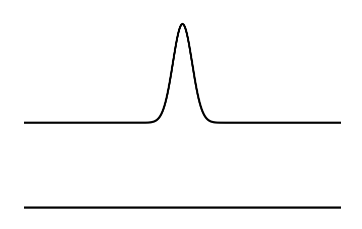
Figure 1: Initial condition for the three experiments. In this and subsequent plots, the upper plot is stress and the lower plot is velocity.

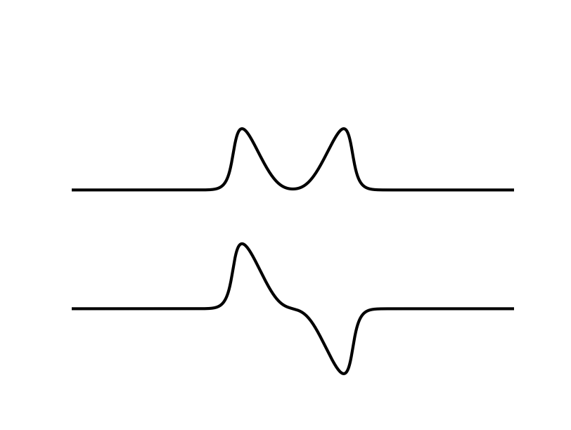
(a) Solution at $t=60$

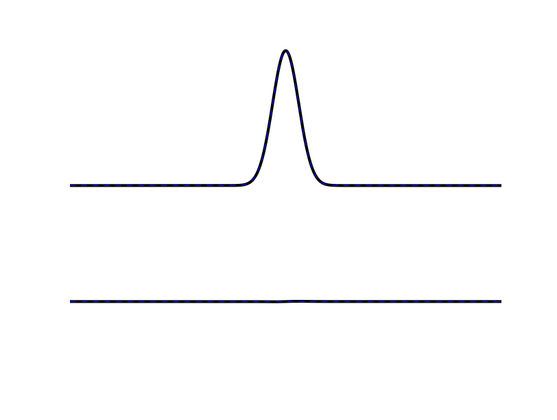
(b) Solution at $t=120$

Figure 2: Stress (upper plot) and velocity (lower plot) snapshots of experiment 1, in which no shocks form. The final solution is identical to the initial condition.

In the second experiment, again $\rho(x)=K(x)=1$ but now the solution is evolved to a much later time. As shown in Figure 3(a), by this time the left- and right-going pulses have developed shocks. Again the velocity is reversed and the solution is evolved for the same length of time. In this case the final solution, shown in Figure 3(b) is quite different from the initial condition.

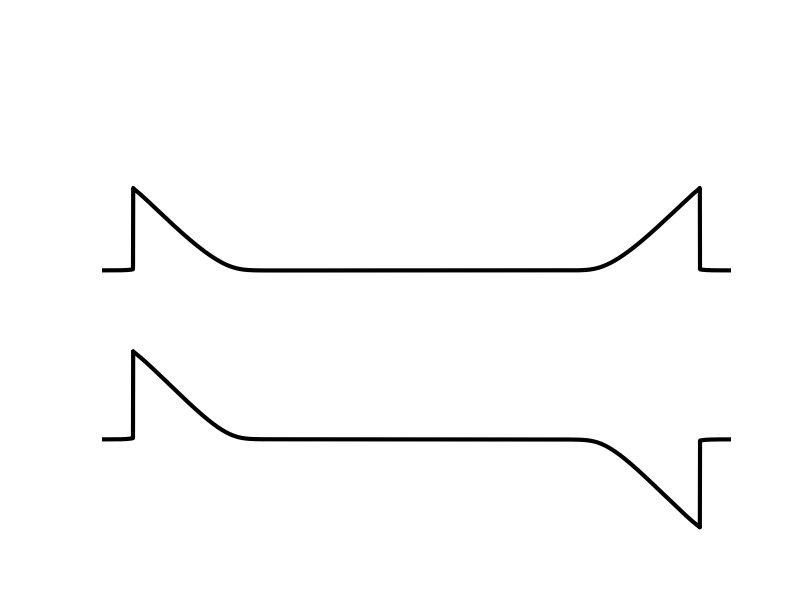
(a) Solution at $t=250$

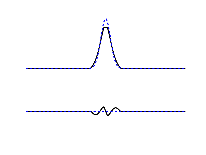
(b) Solid line is solution at $t=500$; dotted line is initial condition

Figure 3: Stress and velocity snapshots of experiment 2, in which shocks form.

In the third experiment, the medium is taken to be periodic and piecewise constant, composed of alternating homogeneous layers of materials A and B, as described by (4), with $\rho_{A}=K_{A}=1$ and $\rho_{B}=K_{B}=4$. The solution is evolved to the same time as in experiment two above. This time, highly oscillatory fronts develop, as shown in Figure 4. Once again the velocity is reversed and the solution evolved for the same length of time. In this case the final solution appears identical to the initial condition.

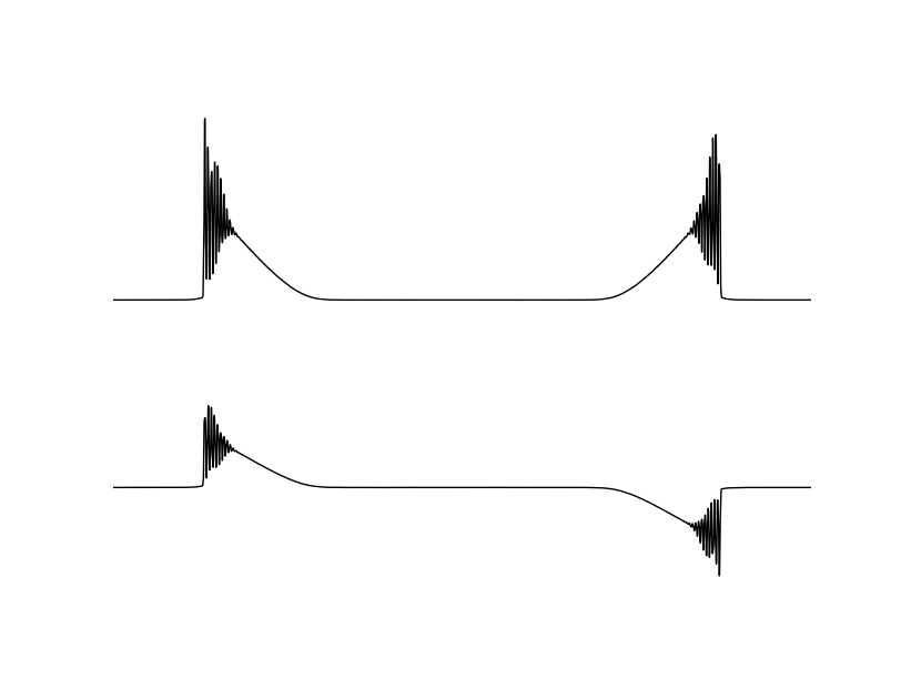
(a) Solution at $t=250$

(b) Solution at $t=500$

Figure 4: Stress and velocity snapshots of experiment 3, in a periodic medium. The final solution is identical to the initial condition.

1.2 First-order hyperbolic systems theory

The results of the first two experiments are well understood within the existing mathematical theory of hyperbolic conservation laws. The system (1) is time-reversible as long as the solution remains smooth. In the first experiment, since shocks do not form, the solution satisfies the nonlinear wave equation (1) in a strong sense and is time-reversible. In the second experiment, characteristics meet and shocks form, leading to a loss of information. In fact, whereas the initial condition we have used is the only one that leads to the solution shown in Figure 2(a) at the given time, there are infinitely many initial conditions that lead to the solution shown in Figure 3(a); the curves in Figure 3(b) are two of them. In general, such irreversible behavior is expected whenever the solution is evolved past the time of shock formation. Thus, from the point of view of the classical theory for nonlinear hyperbolic systems, the long-time reversibility of waves in the periodic medium observed in the third experiment seems remarkable. Similar waves in a homogeneous medium composed of material A or material B would not be reversible at this late time.

1.3 Dispersive nonlinear wave theory

It was shown in [11] that for linear waves whose wavelength is long relative to the period of the medium, the leading order effect of material periodicity is an effective dispersion. Correspondingly, dispersive wave equations are often introduced to model the effect of periodic microstructure [10]. Indeed, a system of dispersive effective equations for the elasticity system (1) with periodic coefficients was derived in [9] and shown to agree with results from direct simulation. Dispersive nonlinear wave equations lead to the appearance of so-called dispersive shock waves, consisting of a high-amplitude oscillatory front followed by a more slowly varying tail [2]. The waves in Figure 4 strongly resemble these dispersive shocks. In such systems, the dispersive term(s) in the equation can often be shown to regularize the solution, preventing the appearance of discontinuities. Hence time-reversibility is typically a property of such dispersive nonlinear systems.

However, the effective dispersive equations of [9], like many dispersive continuum models, rely on an assumption that the wavelength of the solution is large relative to the period of the medium. Since nonlinearity leads to the appearance of high frequencies in the solution, it seems at least possible that this model will break down. One may ask, then, whether true shocks (discontinuities) may indeed appear.

The answer to this question turns out to be quite interesting. As suggested already by the third experiment above, it appears that shocks do not form, even after very long times so long as the amplitude of the initial conditions is not too large relative to the effective dispersion induced by material periodicity. Furthermore, initial shocks with small amplitude appear to be unstable and vanish after a short time. For larger-amplitude solutions, (or weaker effective material dispersion) shock discontinuities appear and persist. Empirically, we find an approximate condition discriminating between data that will or will not lead to shocks, in the form of a characteristic condition that can be seen as a generalization of the well-known Lax entropy condition for shock admissibility.

In the remainder of this section, we describe briefly the numerical methods used in this work. In Section 2, we discuss the problem of detecting shock formation and propose two robust computational approaches. Along the way, we make some observations about limiters used in high-resolution shock-capturing methods. In Section 3, we hypothesize a condition for shock formation in solutions of the nonlinear wave equation (1) in the presence of a periodic medium and conduct some further numerical tests for layered media that support the proposed condition. In Section 4, we discuss the significance of the results and possible generalizations.

The results presented here can be understood even better when accompanied by animations of the wave behavior described. These are available online, along with all code for reproducing the computational results described, at http://bitbucket.org/ketch/layeredmediashocks/src. The reader is highly encouraged to view the animations and experiment with the simulations.

1.4 Numerical discretization

Before continuing, we briefly describe the numerical methods used for the computations presented in this work. The methods employed are both finite volume Godunov-type high-resolution methods, which employ Riemann solvers and nonlinear limiters to obtain good resolution of shocks or steep gradients without spurious oscillations.

The first method used is that implemented in Clawpack [8] and described in [7]. Briefly, this is a second-order TVD high-resolution scheme based on Lax-Wendroff discretization with limiters.

The second method used is that implemented in the SharpClaw software package [4] and described in [5, 6]. This involves a method-of-lines discretization approach, using WENO reconstruction in space and high order Runge-Kutta time integration. In all experiments with SharpClaw we use the fourth-order SSP Runge-Kutta scheme of [3] and fifth-order WENO reconstruction.

2 Computational Measures of Shock Formation

It is clear, at least in the case of a piecewise homogeneous medium, that at least some kinds of smooth initial data will lead to shocks, regardless of the material parameters. For instance, if the initial data includes sufficiently large gradients, certain characteristics will intersect before they reach a material interface. In fact, for any fixed medium it is possible to construct initial data of arbitrarily small amplitude for which a shock forms in the solution. To construct such data, choose a point $x_{0}$ so that $\sigma(\epsilon,x)$ is continuous in $x$ in an open neighborhood about $x_{0}$ and take data

$$\epsilon(x,-\tau) =\begin{cases}\epsilon_{0}&\text{for}~{}x<x_{0}\\ 0&\text{for}~{}x\geq x_{0},\end{cases}$$ (6a)

$$u(x,-\tau) =\begin{cases}-\epsilon_{0}\sqrt{\frac{\sigma^{\prime}(\epsilon_{0})}{\rho(x_{0})}}&\text{for}~{}x<x_{0}\\ 0&\text{for}~{}x\geq x_{0}\end{cases}$$ (6b)

at some very small negative time $-\tau$ with $0<\tau\ll 1$. This data contains a jump discontinuity that spreads out as a 1-rarefaction wave, so that solving up to time $t=0$ gives smooth functions $\epsilon(x,0)$ and $u(x,0)$. Now negate $u(x,0)$ and consider the resulting functions as data at $t=0$. By time-reversibility, over the time $0\leq t\leq\tau$ the solution sharpens back into the discontinuity we started with, corresponding to shock formation.

However, the fact that we can construct data resulting in shock waves does not preclude the possibility that smooth solutions exist for all time for some restricted set of initial data.

Detecting the formation of shocks in computed solutions is challenging, since the computation produces only a finite number of values (cell-averages in the case of the finite volume methods used here) and in general it is impossible to determine if the solution is smooth based on these values. In practice, one can only expect to obtain an upper-bound on the magnitude of possible discontinuities. In [12], visual detection of shocks in spectral solutions was conducted by looking for highly oscillatory regions near steep gradients (evidence of the Gibbs phenomenon). Since the solutions we are interested in contain highly oscillatory regions and steep smooth regions, inspection of the solution may not be a reliable way to judge whether shocks have formed. We propose a more robust and quantitative approach based on two signatures of shock formation. The first, mentioned already in the introduction, is the loss of time-reversibility. The second is entropy decay. We now describe the design of experiments that can detect these signatures.

2.1 Time Reversal

Solutions of hyperbolic systems are time-reversible as long as shocks do not form. This can be used as a computational tool to probe regularization, following the approach used already in the experiments of Section 1:

1. Begin with smooth initial data $q_{0}$.

2. Numerically solve (1) up to time $T$ to obtain a solution $q_{T}$.

3. Reverse the sign of the velocity $u$, to obtain a new solution $q_{0}^{*}$.

4. Numerically solve (1) from time $T$ to time $2T$ with initial condition $q_{0}^{*}$ to obtain a solution $q_{T}^{*}$.

5. If no shocks formed, the solution $q_{T}^{*}$ should match $q_{0}$, up to numerical errors.

As a demonstration, consider the problem from [9], which we will call the LY problem henceforth. This problem is defined as follows. We consider the exponential stress relation (5), and the layered medium defined by (4) with $\rho_{A}=K_{A}=1\mbox{ and }\rho_{B}=K_{B}=4$. An initial pulse is generated by motion of the left boundary:

$$u(0,t) =\begin{cases}-0.1(1+\cos(\pi(t-10)/10))&\mbox{for }0\leq t\leq 20\\ 0&\mbox{for }t>20.\end{cases}$$

After a short time, periodic boundary conditions are imposed in order to observe the long-time behavior of the pulse without using an excessively large computational domain. The initial half-cosine pulse evolves into a train of solitary waves, as shown in Figure 5.

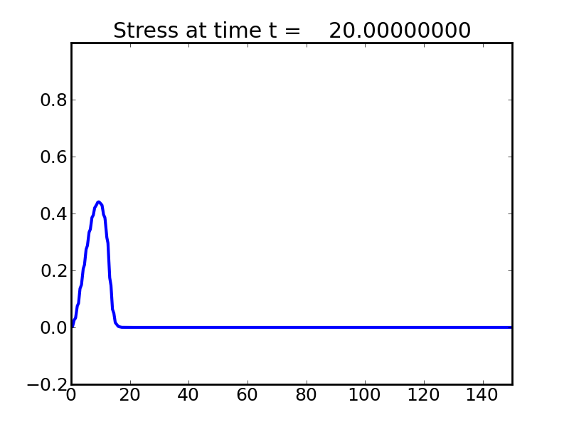
(a) Initial pulse

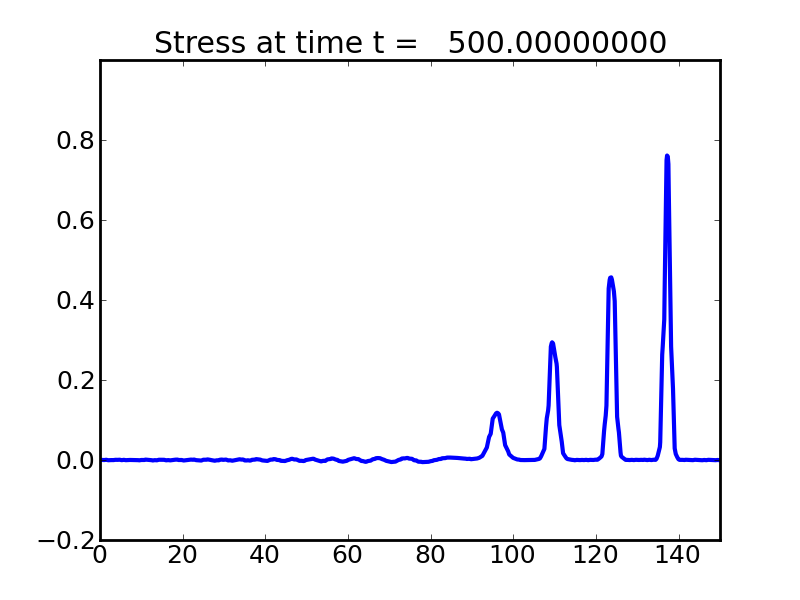
(b) Separation into solitary waves

Figure 5: Evolution of a single pulse into a solitary wave train.

We use the solution to the LY problem at $t=40$ as initial data, solving up to $T=600$, reversing the velocity, and solving again up to time $1160$. The solutions at these two times, plotted in Figure 6(b), appear nearly identical. Indeed, the maximum pointwise difference of the initial and final velocities,

$$E=\|u(x,1160)-u(x,40)\|_{\infty},$$ (7)

which we refer to as the discrepancy, is quite small. In Figure 6(a) we plot the solution obtained using the SharpClaw software [5] on a grid with 24 cells per layer. The $t=1160$ solution (blue squares) is in excellent agreement with the $t=40$ solution (black line). For comparison we also show a solution obtained using Clawpack on the same grid (24 cells per layer), in Figure 6(b). Clawpack uses second order accurate methods with limiters, and gives a less accurate (but also less computationally expensive) solution on the same grid.

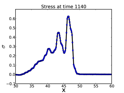
(a) SharpClaw

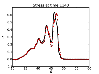
(b) Clawpack

Figure 6: Comparison of forward solution (black line) and time-reversed solution (symbols).

In general the maximum error $E$ is small; We would like to verify that the difference between initial and final solutions is purely due to numerical errors, and not due to the formation of (time-irreversible) shocks. We thus consider the rate at which $E$ decreases as the grid is refined, using the two different numerical methods. Table 1 lists the discrepancy $E$ obtained for a range of grids with both Clawpack and SharpClaw. By using finer grids, both solutions appears to converge to the early time solution. The convergence rate of the SharpClaw scheme fluctuates considerably, and ongoing work is aimed at understanding this.

	Clawpack		SharpClaw
N	$E$	Rate	$E$	Rate
12	$4.36\times 10^{-1}$	-	$5.89\times 10^{-1}$	-
24	$8.15\times 10^{-2}$	2.42	$8.14\times 10^{-3}$	6.18
48	$1.54\times 10^{-2}$	2.40	$9.81\times 10^{-4}$	3.05
96	$3.29\times 10^{-3}$	2.23	$3.72\times 10^{-4}$	1.40
192	$7.41\times 10^{-4}$	2.15	$7.86\times 10^{-5}$	2.24

Table 1: Maximum pointwise discrepancy ($E$ defined in 7) for time-reversal test using Clawpack and Sharpclaw. The quantity $N$ is the number of computational cells per layer of the medium.

Next we conduct the same test but with a less-strongly varying medium, taking $\rho_{B}=K_{B}=Z_{B}=2$. Figure 7 shows the results obtained with SharpClaw using 24 and 48 cells per layer. Observe the large difference between the initial and final solutions. This seems to indicate that shock formation has occurred in this case, leading to a loss of time-reversibility.

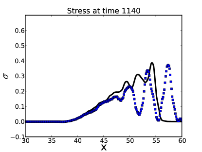
(a) 24 cells per layer

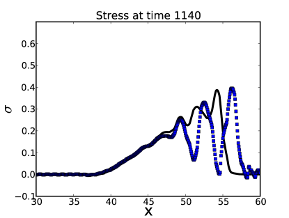
(b) 48 cells per layer

Figure 7: Comparison of forward solution (solid line) and time-reversed solution (dotted line) obtained with SharpClaw using 24 and 48 cells per layer, for an LY medium with lower impedance contrast $Z_{B}=2$. The solution seems not to be time-reversible.

2.2 Entropy Evolution

Another way to detect the formation of shocks computationally is by measuring entropy. An entropy function for (1) is the total energy:

$$\eta(u,\epsilon,x)=\frac{1}{2}\rho(x)u^{2}+\int_{0}^{\epsilon}\sigma(s,x)ds.$$ (8)

It is straightforward to see that $\eta$ is conserved for smooth solutions:

$$\frac{d}{dt}\int_{-\infty}^{\infty}\eta dx =\int_{-\infty}^{\infty}\eta_{t}dx$$

$$=\int_{-\infty}^{\infty}\left(\rho(x)uu_{t}+\frac{d}{dt}\int_{0}^{\epsilon(x,t)}\sigma(s,x)ds\right)dx$$

$$=\int_{-\infty}^{\infty}\left(\rho uu_{t}+\sigma(\epsilon,x)\epsilon_{t}\right)dx$$

$$=\int_{-\infty}^{\infty}\left(u\sigma_{x}+\sigma u_{x}\right)dx=\int_{-\infty}^{\infty}(\sigma u)_{x}dx=0.$$

However, when shocks form the entropy of the physically correct vanishing-viscosity solution will decrease. Since our numerical methods are designed to compute the vanishing-viscosity solution, the numerical entropy will also tend to decrease when shocks form. In this section we study the evolution of entropy in computational solutions.

In Figure 8, we show the evolution of entropy over time for an initial gaussian stress perturbation in a medium with $\rho_{A}=K_{A}=1$ and $\rho_{B}=K_{B}=Z_{B}$, for varying values of $Z_{B}$. In each case, the entropy is normalized to be unity at time zero. The case $Z_{B}=1$ corresponds to a homogeneous medium, and the entropy decays rapidly once a shock forms. For $Z_{B}=2$, the entropy evolution indicates that shock formation is delayed and the resulting shocks are weaker. For $Z_{B}=4$, the entropy is nearly constant over the duration of the simulation.

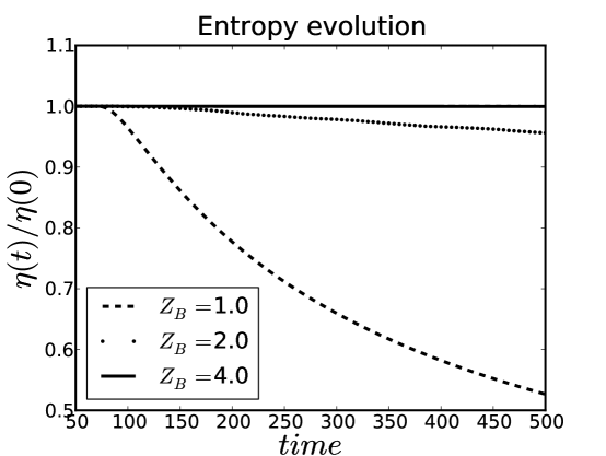
Figure 8: Entropy evolution in time for media with various impedance ratios. In this test, the density and bulk modulus of layer B were varied simultaneously and are equal to $Z_{B}$ in each case.

Numerical dissipation can also lead to a loss of entropy in the computational solution. Using a first-order method, the entropy evolution is entirely dominated by this effect. For the higher order numerical methods employed in this paper, we have found that entropy may numerically increase or decrease depending on how agressive the limiter is. Overcompressive numerical limiters can lead to (unphysical) entropy production. However, all numerical effects on entropy evolution appear to decrease rapidly with grid resolution, as shown in Figure 9, which indicates the relative entropy loss versus grid resolution at $T=500$ for $Z_{B}=4$. Among the limiters implemented in Clawpack, the smallest change in entropy is generally produced by the van Leer limiter (for sufficiently fine grids). The van Leer limiter is used in all subsequent Clawpack simulations in this paper. Using SharpClaw with fifth-order WENO reconstruction, we find that the entropy errors are much smaller than for any of the Clawpack limiters, especially on the finer grids.

We remark that this test might be taken as a measure of the dissipativity of a given limiter. For instance, note that the results in Figure 9 for Minmod and Superbee suggest that they are dissipative and over-compressive, respectively. It is interesting to note that, by this measure, the MC limiter is somewhat over-compressive, while the van Leer limiter is somewhat dissipative. Fifth-order WENO is neutrally-compressive. That is, the entropy fluctuates slightly around the initial value, but is roughly constant in time if averaged over short intervals.

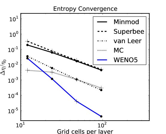
Figure 9: Entropy change up to $T=500$ versus number of grid cells per medium layer for the four limiters implemented in Clawpack. Here $Z_{B}=4$. Plus signs (’+’) indicate cases for which the entropy has increased, while filled circles indicate cases for which the entropy has decreased.

Due to numerical dissipation (or compression), it is impossible to completely rule out physical loss of entropy. Instead, we can bound the possible loss of entropy through use of very fine spatial resolution. For sufficiently fine grids, we have noticed that the small numerical entropy fluctuations are nearly time-reversible. That is, if we run the time-reversibility experiment of the last section and consider the entropy at corresponding early and late times, the difference is much smaller than the (already small) difference between the entropy at either time and the initial entropy. This allows us to probe the degree to which entropy is conserved for different impedance contrasts.

In Figure 10, we plot the difference in entropy values at times $t=50$ and $t=450$ (using a final time of $T=500$), for SharpClaw solutions on fine grids. We observe that the change in entropy generally gets smaller as the impedance contrast increases and as the resolution of the simulation increases. For a given grid, the entropy change apparently diminishes until it reaches the level of numerical errors. For impedance contrast greater than 2.5, the entropy change on the finest grid is less than $10^{-7}$. Similar results are obtained with Clawpack, although much finer resolution is required to resolve the small losses of entropy [1].

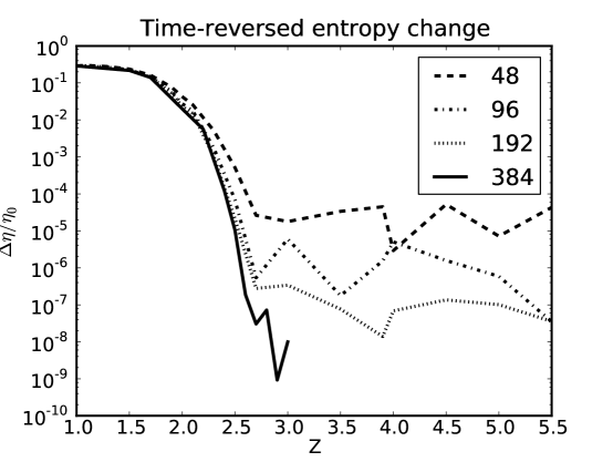
Figure 10: Change in entropy for LY media with increasing impedance contrast. The different plots correspond to differing spatial resolutions; the number of cells per material layer is indicated in the legend.

3 A Condition for Shock Formation in Heterogeneous Media

In this section we hypothesize and test a condition for shock formation. This condition is empirically motivated, but leads to quantitatively accurate predictions and can be motivated by simple arguments.

We will make use of the arithmetic and harmonic averaging operators, denoted by a bar and a hat, respectively:

$$\bar{f} =\int_{0}^{1}f(x)dx \hat{f} =\left(\int_{0}^{1}\frac{1}{f(x)}dx\right)^{-1}.$$

3.1 Effective wave speeds

In a homogeneous medium, small-amplitude perturbations travel at the characteristic speed

$$c(\sigma_{0})=\sqrt{\frac{\sigma^{\prime}_{0}(\epsilon)}{\rho}}\ \ \ \mbox{ where }\sigma^{\prime}_{0}(\epsilon)=\left.\sigma^{\prime}(\epsilon)\right|_{\sigma=\sigma_{0}},$$

where $\sigma_{0}$ is the stress in the ambient state. In particular, in the linear case these velocities are equal to the sound speed:

$$\sigma(\epsilon) =K\epsilon\implies c=\sqrt{K/\rho}.$$ (9)

Now let us consider a linear periodic medium. A pulse in such a medium will spread out over time due to reflections. The fastest moving part is that which is unreflected; this part travels at the harmonic average of the sound speed:

$$\hat{c}=\left(\int_{0}^{1}{\sqrt{\frac{\rho(x)}{K(x)}}dx}\right)^{-1}.$$ (10)

Meanwhile, the main part of the signal (for a long-wavelength pulse) travels at the effective sound speed given by using the average of the density and the harmonic average of the bulk modulus [11]:

$$c_{\textup{eff}}=\sqrt{\frac{\hat{K}}{\bar{\rho}}}$$ (11)

The effective velocity (11) is smaller than the maximum bulk velocity (10), due to the macroscopic slowing effect of repeated reflections.

By similar reasoning, small-amplitude perturbations traveling in a nonlinear periodic medium with ambient stress $\sigma_{0}$ can be shown to travel at an effective velocity

$$c_{\textup{eff}}(\sigma_{0}) =\pm\sqrt{\frac{\widehat{\sigma^{\prime}_{0}}}{\bar{\rho}}} \mbox{where }\sigma^{\prime}_{0} =\left.\frac{\partial\sigma(\epsilon,x)}{\partial\epsilon}\right|_{\sigma=\sigma_{0}}.$$

Now consider the case of a shock separating two constant states $q_{l},q_{r}$ in the nonlinear medium, and let $[q]$ denote the jump $q_{r}-q_{l}$. Since it will experience reflections at the material interfaces, the shock may conceivably break up into many smaller discontinuities, as it clearly would in the linear case. If the shock is able to persist as a single large discontinuity (due to nonlinear compression), we might expect that it will also travel at an effective velocity; it is natural to suppose that this velocity will be related to the Rankine-Hugoniot shock speed in the same way that the effective velocities above are related to the characteristic speeds. The R-H jump conditions in a homogeneous medium give the shock speed

$$s=\sqrt{\frac{[\sigma]}{[\epsilon]\rho}}.$$ (12)

Thus it is natural (based on (11)) to consider an ”effective shock speed”

$$s_{\textup{eff}}=\sqrt{\widehat{\left(\frac{[\sigma]}{[\epsilon]}\right)}\frac{1}{\bar{\rho}}},$$ (13)

which we propose as an estimation of the velocity at which the largest portion of the jump may travel. Smaller parts of the shock will have spread out due to being reflected more or fewer times. The fastest-travelling portion is that which undergoes no reflections. The strength of this ”purely transmitted” shock diminishes exponentially in time, so that to a good approximation it travels at the speed for non-reflected small perturbations in the state ahead of the shock:

$$\hat{c}(\sigma_{r})=\left(\int_{0}^{1}\left(\frac{\sigma^{\prime}_{r}(x)}{\rho(x)}\right)^{-1/2}dx\right)^{-1}.$$

3.2 A generalized entropy condition

A generalized condition for shock stability can be motivated as follows. The bulk of the shock will advance at speed $s_{\textup{eff}}$. If $s_{\textup{eff}}<\hat{c}(\sigma_{r})$ then the bulk of the shock will fall behind the leading (weak) bit. This will make the main shock weaker, causing it to propagate even more slowly, so that more of the strength of the shock will ”escape” ahead of it. Hence the shock will be converted into many weak shocks after some time.

This proposed condition for shock persistence in the periodic medium can be viewed as a generalization of the Lax entropy condition for shocks. Namely, characteristics of the corresponding family must impinge on the shock. In our case, the characteristic speed involved in this condition is the harmonic average of the sound speed ahead of the shock. The relevant shock speed is the effective shock speed $s_{\textup{eff}}$ from (13).

The effective shock speed for various values of $Z_{B}$ (with $\rho_{B}=K_{B}=Z_{B}$) and a range of stresses $\sigma_{l}$ is plotted in Figure 11. Here we have taken $\sigma_{r}=0$, so that $\hat{c}(\sigma_{r})=1$. Hence we expect shock stability for a given impedance $Z_{B}$ and left state $\sigma_{l}$, if the corresponding effective shock speed (13) is greater than unity. For the homogeneous medium ($\rho_{B}=K_{B}=Z_{B}=1$), the effective shock speed is just the ordinary shock speed, and any shock is of course predicted to be stable. However, for heterogeneous media, small-amplitude shocks have effective velocity less than one, so that effective characteristics do not impinge on the shock from the right.

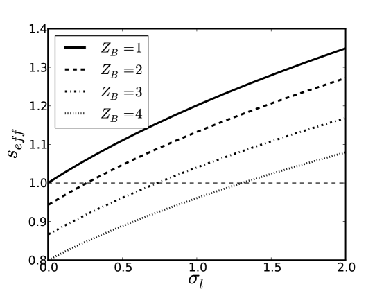
Figure 11: Effective shock speed (13) as a function of stress behind the shock.

Based on the foregoing theory, we can define a critical parameter that we will refer to as the relative effective shock speed:

$$S_{\textup{eff}} =\frac{s_{\textup{eff}}}{\hat{c}(\sigma_{r})}.$$ (14)

Notice that $S_{\textup{eff}}$ depends on the ambient states $\sigma_{r},\sigma_{l}$ as well as the material parameters $\rho(x),\sigma^{\prime}_{r}(x)$. We expect that a shock will form whenever $S_{\textup{eff}}$ exceeds unity.

3.3 Numerical validation

The true dynamics of a propagating front in the periodic medium is generally much more complicated than what we have just considered, since such a front quickly results in many reflected/transmitted shocks and rarefactions in mutual interaction. Nevertheless, simulations of low-contrast media and large-amplitude initial conditions do lead to persistent large-amplitude shock fronts, whereas simulations of higher-contrast media or smaller-amplitude initial conditions such shocks are not visibly apparent. For the former case, we have compared directly the apparent shock velocity with the predicted value $s_{\textup{eff}}$. There is some ambiguity in determining the precise location of the shock, since the front structure is complex, but in general agreement to within 1-3% is observed for the range of materials and initial conditions considered in this work.

We now conduct two tests to quantitatively validate this theory. In the first, we test whether shocks form from smooth initial conditions. The initial condition consists of two uniform initial states separated by a thin smooth transition region. The solution is evolved to time $t=100$, well beyond the time for shock formation in a homogeneous medium for all of the initial states studied. Then the velocity is reversed and the simulation continues to $t=200$. The final entropy and initial entropy are compared to determine whether shock formation has occurred. In Figure 12, the ratio of final and initial entropies is plotted for many tests over the ranges $1.5\leq\rho_{B}\leq 9,1\leq K_{B}\leq 4,0.1\leq\sigma_{l}\leq 4$, and $\sigma_{r}=0$. The results are in very good agreement with the theory; i.e. entropy loss occurs when $S_{\textup{eff}}>1$ and generally is on the level of numerical error otherwise.

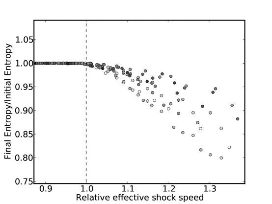
Figure 12: Relative entropy versus relative effective shock speed $S_{\textup{eff}}$ (14) for a wide range of materials and initial conditions. Notice that the entropy is near constant for $S_{\textup{eff}}<1$ (indicating no shock formation), and decreasing for $S_{\textup{eff}}>1$ (indicating shock formation). The shade of each point indicates the impedance contrast on a logarithmic scale, with darker points corresponding to higher impedance contrast.

In the second test, we start with discontinuous initial conditions and study the entropy evolution in time. There is some difficulty in choosing an initial condition. Using a pure right-going shock in one material quickly leads to very strong reflections. Instead, we use an initial condition consisting of an ”effective shock”, where the left and right states are related by the usual Rankine-Hugoniot conditions but with the material parameters $\rho,K$ replaced by the effective parameters $\bar{\rho},\hat{K}$. Specifically, we take $(\sigma(x,0),u(x,0))=0$ for $x>30$ and $(\sigma(x,0),u(x,0))=(\sigma_{l},u_{l})$ for $x\leq 30$, where

$$u_{l} =-\sqrt{\frac{\sigma_{l}\log(\sigma_{l}+1)}{\bar{\rho}\hat{K}}}.$$

This dramatically reduces the severity of initial reflections of the front, which seems advantageous for our purpose of studying shock propagation.

The total entropy evolution versus time is plotted in Figure 13 for a range of values of $\sigma_{l}$ and a medium with $Z_{B}=\rho_{B}=K_{B}=2$. The legend indicates the corresponding values of the relative effective shock speed $S_{\textup{eff}}$. In all cases there is a rapid but small initial entropy loss. However, for $S_{\textup{eff}}<1$ the entropy is nearly constant after this initial time. On the other hand, for $S_{\textup{eff}}>1$ the entropy continues to decrease significantly throughout the simulation.

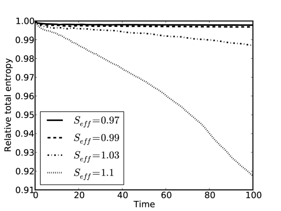
Figure 13: Entropy as a function of time (relative to initial entropy) for a range of relative effective shock speeds $S_{\textup{eff}}$ (14). The medium has $\rho_{B}=K_{B}=Z_{B}=2$. Notice that the entropy is nearly constant (after a brief initial decrease) for $S_{\textup{eff}}<1$, and decreasing for $S_{\textup{eff}}>1$.

Figure 14 shows similar results for a medium with $Z_{B}=\rho_{B}=K_{B}=4$. In this case, we see that for $S_{\textup{eff}}$ slightly less than 1, some significant entropy loss continues after the initial period. The entropy loss is much more significant when $S_{\textup{eff}}>1$.

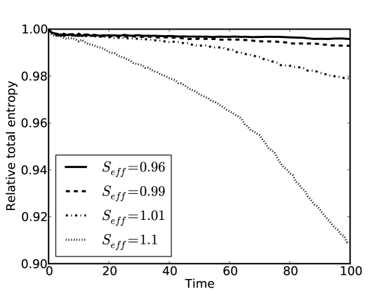
Figure 14: Entropy as a function of time (relative to initial entropy) for a range of relative effective shock speeds $S_{\textup{eff}}$ (14). The medium has $\rho_{B}=K_{B}=Z_{B}=4$. Notice that the entropy is nearly constant (after a brief initial decrease) for $S_{\textup{eff}}<1$, and decreasing for $S_{\textup{eff}}>1$.

4 Discussion

The main findings of this work can be summarized as follows:

1. Layered periodic materials with varying impedance tend to inhibit shock formation.

2. Weak shocks in periodic media are unstable, in the sense that they do not persist as noticeable discontinuities and do not lead to significant long-term entropy decay.

3. Initial perturbations with large enough amplitude do lead to shock formation and substantial sustained entropy decay.

4. The formation of shocks can be quantitatively predicted, to a good approximation, by a generalized characteristic condition.

In order to detect the formation of shocks in layered periodic media, we have studied the time-reversibility and the entropy evolution of computated solutions. Based on these experiments and some intuition, we are led to a simple criterion for shock formation in terms of one parameter: the relative effective shock speed $S_{\textup{eff}}$. This theory is consistent with a wide range of experiments involving simple layered media. It also seems to be a natural generalization of the Lax entropy condition, taking into account the effective properties of the periodic medium.

This result has potentially important implications both for nonlinear hyperbolic PDE theory (the fact that shocks appear to be avoided for all time when $S_{\textup{eff}}<1$) and for effective medium theory (the fact that classical shocks may still form in a periodic medium when $S_{\textup{eff}}>1$). The result has been formulated in terms of general periodic media and could be interpreted in a natural way for other heterogeneous (non-periodic) media. Whether the same condition for shock formation holds in such broader settings is an open question. Another way in which this theory could be generalized naturally involves application to more general first-order hyperbolic systems. Both of these topics are the subject of ongoing research.

A very interesting question touched on in the introduction is that of whether it is possible for non-trivial initial conditions to remain smooth for all time in the solution of nonlinear hyperbolic PDEs with varying coefficients. Because the approach of the present work has been based on computation and observation, it provides tantalizing hints but does not address in a strict way the answer to this question.

We finally remark that the interesting behavior of different limiters with respect to entropy evolution for the waves studied here seems worthy of further study.

Acknowledgments

This research was supported in part by NSF grant DMS-0914942 and NIH grant 5R01AR53652-2.

References

- [1] A. Alghamdi, A. Ahmadia, D. Ketcheson, M. Knepley, K. Mandli, and L. Dalcin, PetClaw: A Scalable Parallel Nonlinear Wave Propagation Solver for Python, ACM, 2011. To appear in proceedings of HPC 2011.
- [2] G. a. El, Resolution of a shock in hyperbolic systems modified by weak dispersion., Chaos (Woodbury, N.Y.), 15 (2005), p. 37103.
- [3] D. I. Ketcheson, Highly Efficient Strong Stability Preserving Runge-Kutta Methods with Low-Storage Implementations, SIAM Journal on Scientific Computing, 30 (2008), pp. 2113–2136.
- [4] D. I. Ketcheson, SharpClaw software, 2011.
- [5] D. I. Ketcheson and R. J. LeVeque, WENOCLAW: A higher order wave propagation method, in Hyperbolic Problems: Theory, Numerics, Applications: Proceedings of the Eleventh International Conference on Hyperbolic Problems, Berlin, 2008, p. 1123.
- [6] D. I. Ketcheson, M. Parsani, and R. J. LeVeque, High-order wave propagation algorithms for general hyperbolic systems. 2011.
- [7] R. J. LeVeque, Wave Propagation Algorithms for Multidimensional Hyperbolic Systems, Journal of Computational Physics, 131 (1997), pp. 327–353.
- [8] R. J. LeVeque and M. J. Berger, Clawpack Software version 4.5, 2011.
- [9] R. J. LeVeque and D. H. Yong, Solitary waves in layered nonlinear media, SIAM Journal of Applied Mathematics, 63 (2003), pp. 1539–1560.
- [10] M. Rubin, P. Rosenau, and O. Gottlieb, Continuum model of dispersion caused by an inherent material characteristic length, Journal of Applied Physics, 77 (2009), pp. 4054–4063.
- [11] F. Santosa and W. Symes, A dispersive effective medium for wave propagation in periodic composites, SIAM Journal of Applied Mathematics, 51 (1991), pp. 984–1005.
- [12] G. Simpson and M. I. Weinstein, Coherent Structures and Carrier Shocks in the Nonlinear Periodic Maxwell Equations, (2010).