We study the entanglement dynamics of two non-interacting, spatially separated qubits subject to local environment noises. Based on exactly solvable models for non-Markovian amplitude damping and phase damping noises, we are able to analyze the entanglement dynamics of the two qubits for different coupling bandwidths and different detunings. We show that entanglement oscillations can occur for both amplitude and phase damping noises. Moreover, we demonstrate that changing the coupling bandwidth can lead to crossover between dissipative and non-dissipative entanglement dynamics, while varying the detuning controls the crossover between strong and weak coupling limits. Our findings can help provide a synthesized picture for the entanglement dynamics of two qubits subject to local environment noises.

PACS numbers: 03.65.Ud, 03.65.Yz, 03.67.Mn

Keywords: quantum entanglement, non-Markovian dynamics, two qubits, crossover

I. Introduction

Advancements of quantum information sciences during the past few decades have been bringing new lights into researches on the fundamental issues of quantum mechanics [1]. Among them, studies of entanglement dynamics for open quantum systems have occupied a central part due to the crucial role of quantum entanglement in many aspects of quantum information sciences [2]. For general multi-qubit systems, the study of entanglement dynamics remains a major challenge due to the lack of a manageable quantitative measure for entanglement in such systems [3]. In the case of two-qubit systems, however, there have been reliable and easily computable entanglement measures which have greatly assisted investigations of entanglement dynamics in these systems. In particular, the degradation of entanglement in two-qubit systems in the presence of environment noises has been an issue of great theoretical and experimental interests [4].

In this paper, we shall examine the entanglement dynamics of two spatially separated, non-interacting qubits subject to local environment noises. This may correspond to, for instance, a pair of entangled two-level atoms located in two different (lossy) cavities, where each atom is separately coupled to the cavity modes. In order to study the entanglement evolution of the qubits under the action of environment noises, we will consider the cases of amplitude damping noise, which can cause energy relaxations in the qubits, and of phase damping noise, which can degrade the phase coherence of the qubits [1]. The Markovian dynamics of the qubit entanglement for such systems have been studied extensively [4]. Novel effects such as the complete destruction of entanglement within finite time (the entanglement sudden death) have been predicted and observed experimentally [4, 5, 6, 7]. There have also been researches on the non-Markovian entanglement dynamics in such systems. In particular, entanglement oscillations due to the finite memory time of the environment coupling have been predicted theoretically for amplitude damping noise [8, 9], and observed experimentally in photonic systems [10]. In this paper, based on analytically solvable models that exhibits non-Markovian characteristics, we will show that for both amplitude damping and phase damping noises, crossovers between oscillatory and monotonic decaying entanglement evolution can occur in connection with the transition between the non-dissipative and dissipative limits of the environment coupling, which may also be regarded as a crossover between the non-Markovian and the Markovian limits. Furthermore, our model shall also enable us to examine the crossover between the limits of weak and strong environment couplings. Therefore, our results demonstrate not only that entanglement oscillations can occur also for two qubits under phase damping noises (cf. Ref. [11]), but also offer detailed analysis for the entanglement dynamics of two qubits in various regimes which can help provide a synthesized view for the related problems. It should be noted, however, that here our emphasis will lie in the entanglement dynamics of the qubits, rather than the different measure(s) for the “non-Markovianity” of the dynamical maps that we will discuss [12, 13, 14]; even though there are connections between the two (see later). In other words, it is the physical reasons behind the appearance/disappearance of entanglement oscillations that will concern us, instead of any specific quantitative measure for the “non-Markovianity” of the dynamical processes.

We will begin in the following section by a brief summary for our theoretical framework. On the basis of Kraus representation [15], we shall explain how the dynamics of two independent qubits can be constructed based on the single-qubit dynamics. Then in Secs. III. and IV. we will apply this formulation to examine the non-Markovian dynamics of two qubits subject to, respectively, amplitude damping and phase damping noises. Finally, Sec. V. provides a summary of our results and some further discussions.

II. Theoretical formulation

Let us consider two spatially separated qubits that are interacting with their local environments independently from each other. We shall model the environment as a wide spectrum of harmonic oscillator modes so that for each qubit the total Hamiltonian reads (we shall take $\hbar=1$ throughout)

$$H=\frac{\omega_{0}}{2}\sigma_{z}+\sum_{k}\omega_{k}b_{k}^{\dagger}b_{k}+H_{I}\,.$$ (1)

Here $\omega_{0}$ is the energy separation between the qubit levels $|\pm\rangle$ (which have energies $\pm\frac{\omega_{0}}{2}$, respectively), $\sigma_{z}$ is the third Pauli matrix, and $b_{k}$ is the annihilation operator for the oscillator mode with frequency $\omega_{k}$ in the environment degrees of freedom. The last term $H_{I}$ in (1) denotes the interaction Hamiltonian for the qubit and its local environment, whose explicit form will be specified later. Since the two qubits are not interacting with each other and their environment noises are uncorrelated, the two-qubit dynamics can be constructed from the single-qubit dynamics based on the Kraus formulation, as we shall now explain [5].

For the single-qubit Hamiltonian (1), suppose one can find the time evolution for the reduced density matrix $\tilde{\rho}$, it is then possible to express [15]

$$\tilde{\rho}(t)=\sum_{i=1}^{2}E_{i}\tilde{\rho}(0)E_{i}^{\dagger}\,,$$ (2)

where $\tilde{\rho}(0)$ is the initial density matrix for the qubit and $E_{i}$ are the operation elements associated with the time evolution of the qubit. These operation elements are encoded with effects of the environment noises on the qubit and satisfy $\sum_{i=1}^{2}E_{i}^{\dagger}E_{i}=1$ [15]. Once the single-qubit operation elements are known, the time evolution of two independent qubits $A$, $B$ can then be obtained from the operation elements [5]

$$K_{1}=E_{1}^{A}\otimes E_{1}^{B}\,,$$

$$K_{2}=E_{1}^{A}\otimes E_{2}^{B}\,,$$

$$K_{3}=E_{2}^{A}\otimes E_{1}^{B}\,,$$

$$K_{4}=E_{2}^{A}\otimes E_{2}^{B}\,,$$ (3)

where the superscripts $A$, $B$ are the qubit labels. The reduced density matrix $\rho$ for the two qubits thus evolves according to

$$\rho(t)=\sum_{i=1}^{4}K_{i}\rho(0)K_{i}^{\dagger}\,$$ (4)

with $\rho(0)$ the initial density matrix for the two qubits. Applying this formulation, in the following sections we shall consider specific models for the system-environment interaction $H_{I}$ for which the operation elements can be found explicitly. We will consider two types of environment noises separately: the amplitude damping noise, which can cause energy relaxations in the qubits, and the phase damping noise, which can lead to dephasing in the qubits [1]. Based on these results, we shall study the time evolution of the two-qubit entanglement.

III. Amplitude damping

A. Single-qubit dynamics

As our first case for the qubit-environment coupling, let us consider a single qubit interacting with the environment by absorbing and emitting energy quanta from the oscillator modes, and at the same time making transitions between the upper and lower qubit levels. This interaction would thus change the level occupations in the qubit and cause energy relaxations (thus frequently termed the amplitude damping channel). We model this coupling by using the following interaction Hamiltonian in (1) [16]

$$H_{I}=\sum_{k}\left(g_{k}\sigma_{-}b_{k}^{\dagger}+g_{k}^{*}\sigma_{+}b_{k}\right)\,,$$ (5)

where $g_{k}$ are the coupling constants and $\sigma_{\pm}$ are the raising/lowering operators for the qubit levels. The time evolution of the qubit in the presence of the coupling (5) can be solved exactly [17] and the corresponding operation elements in the basis $\{|+\rangle,|-\rangle\}$ are

$$E_{1}=\left(\begin{array}[]{cc}p&0\\ 0&1\end{array}\right)\,,\quad E_{2}=\left(\begin{array}[]{cc}0&0\\ q&0\end{array}\right)\,,$$ (10)

where $q\equiv\sqrt{1-|p|^{2}}$. Here $p$ is the solution for the equation

$$\frac{d}{dt}p(t)=-\int_{0}^{t}d\tau f(t-\tau)p(\tau)$$ (11)

with $f$ the noise correlation function [16]

$$f(t-\tau)$$ (12)

$$\equiv \left\langle\left(\sum_{k}g_{k}^{*}b_{k}e^{-i\omega_{k}t}\right)\left(\sum_{k^{\prime}}g_{k^{\prime}}b_{k^{\prime}}^{\dagger}e^{i\omega_{k^{\prime}}\tau}\right)\right\rangle\,e^{i\omega_{0}(t-\tau)}$$

$$= \sum_{k,k^{\prime}}g_{k}^{*}g_{k^{\prime}}\langle b_{k}b_{k^{\prime}}^{\dagger}\rangle\,e^{i(\omega_{0}-\omega_{k})t}\,e^{-i(\omega_{0}-\omega_{k^{\prime}})\tau}\,.$$

The expectation values in (12) are taken with respect to the state of the environment. For our calculation, we shall consider a vacuum initial environment state. Thus the noise correlation function (12) reduces to

$$f(t-\tau) = \sum_{k}|g_{k}|^{2}\,e^{i(\omega_{0}-\omega_{k})(t-\tau)}$$ (13)

$$= \int_{-\infty}^{\infty}d\omega\,J(\omega)\,e^{i(\omega_{0}-\omega)(t-\tau)}$$

with $J(\omega)$ the spectral function for the coupling [16]. In the following, we will consider a specific form for the spectral function that shall enable analytic solution for (11). The single qubit dynamics can thus be attained explicitly.

Let us consider a Lorentzian spectral function for the qubit-environment coupling [13]

$$J(\omega)=\frac{1}{2\pi}\frac{\gamma\lambda^{2}}{(\omega-\omega_{0}+\Delta)^{2}+\lambda^{2}}\,.$$ (14)

Here $\gamma$ is the (phenomenological) decay rate for the upper qubit level $|+\rangle$, $\lambda$ is the bandwidth of the coupling (thus $\lambda^{-1}$ characterizes the environment coherence time), and $\Delta$ is the detuning from the resonance frequency $\omega_{0}$. Utilizing (14) in (13), one can obtain the correlation function $f$ easily and then solve for $p(t)$ from (11). One finds [9]

$$p(t)=e^{-\left(\frac{\lambda-i\Delta}{2}\right)t}\left[\cosh\left(\frac{dt}{2}\right)+\frac{\lambda-i\Delta}{d}\sinh\left(\frac{dt}{2}\right)\right],$$ (15)

where

$$d\equiv\sqrt{(\lambda-i\Delta)^{2}-2\gamma\lambda}\,.$$ (16)

With the explicit form for the function $p$, one can construct the operation elements in (10). Following the prescriptions of Sec. II. we are now ready for studying the two-qubit dynamics.

B. Two-qubit dynamics

Let us now consider two non-interacting qubits that are coupled to independent amplitude damping noises separately, each described by (5). With the results for single qubit dynamics in the preceding subsection, as described in Sec.II. one can obtain the two-qubit operation elements $K_{i}$ using (10) and (15) in (3). The time evolution of the reduced density matrix for the two qubits then follows from (4). Using the basis $\{|++\rangle,|+-\rangle,|-+\rangle,|--\rangle\}$, we find the matrix elements [9]

$$\rho_{11}(t) = |p_{A}\,p_{B}|^{2}\rho_{11}(0)\,,$$

$$\rho_{22}(t) = |p_{A}|^{2}\left(\rho_{22}(0)+q_{B}^{2}\,\rho_{11}(0)\right)\,,$$

$$\rho_{33}(t) = |p_{B}|^{2}\left(\rho_{33}(0)+q_{A}^{2}\,\rho_{11}(0)\right)\,,$$

$$\rho_{44}(t) = 1-\left(\rho_{11}(t)+\rho_{22}(t)+\rho_{33}(t)\right)\,,$$

$$\rho_{12}(t) = |p_{A}|^{2}\,p_{B}\,\rho_{12}(0)\,,$$

$$\rho_{13}(t) = p_{A}\,|p_{B}|^{2}\,\rho_{13}(0)\,,$$

$$\rho_{14}(t) = p_{A}\,p_{B}\,\rho_{14}(0)\,,$$

$$\rho_{23}(t) = p_{A}\,p_{B}^{*}\,\rho_{23}(0)\,,$$

$$\rho_{24}(t) = p_{A}\left(\rho_{24}(0)+q_{B}^{2}\,\rho_{13}(0)\right)\,,$$

$$\rho_{34}(t) = p_{B}\left(\rho_{34}(0)+q_{A}^{2}\,\rho_{12}(0)\right)\,.$$ (17)

Here $p_{\alpha}$ (with $\alpha=A,B$ the qubit labels) are given by (15) but with the parameters now carrying the qubit labels, ie. $\gamma\rightarrow\gamma_{\alpha}$, $\lambda\rightarrow\lambda_{\alpha}$, $\Delta\rightarrow\Delta_{\alpha}$ (hence also $d\rightarrow d_{\alpha}$), and as in (10), we denote $q_{\alpha}\equiv\sqrt{1-|p_{\alpha}|^{2}}$.

In order to study the entanglement dynamics of the pair of qubits, we shall adopt concurrence as the entanglement measure [18], namely

$$C(t)=\max\Big{\{}\,0,\sqrt{\mu_{1}}-\sqrt{\mu_{2}}-\sqrt{\mu_{3}}-\sqrt{\mu_{4}}\Big{\}}\,,$$ (18)

where $\mu_{i}$ ($i=1\sim 4$) are eigenvalues of the matrix $\rho(\sigma_{y}^{A}\otimes\sigma_{y}^{B})\rho^{*}(\sigma_{y}^{A}\otimes\sigma_{y}^{B})$ in descending orders; $\sigma_{y}^{\alpha}$ is the second Pauli matrix for qubit $\alpha$. Using (17) and (15), one can find the concurrence evolution for any initial density matrix accordingly. For instance, for an initial density matrix of the “X-form” [19]

$$\rho(0)=\left(\begin{array}[]{cccc}\rho_{11}&0&0&\rho_{14}\\ 0&\rho_{22}&\rho_{23}&0\\ 0&\rho_{32}&\rho_{33}&0\\ \rho_{41}&0&0&\rho_{44}\end{array}\right)\,,$$ (23)

it follows from (17) and (18) that the concurrence for the reduced density matrix $\rho(t)$ is given by

$$C(t)=2\max\Big{\{}\,0, |\rho_{14}(t)|-\sqrt{\rho_{22}(t)\rho_{33}(t)}\,,$$ (24)

$$|\rho_{23}(t)|-\sqrt{\rho_{11}(t)\rho_{44}(t)}\,\Big{\}}\,.$$

In the following, we shall present results based on the calculations outlined above. We will consider symmetric configurations in which the two qubits are identical, so that they have the same level separation $\omega_{0}$ and the same decay rate $\gamma_{A}=\gamma_{B}=\gamma$, and are subject to amplitude noises of identical characteristics, thus $\lambda_{A}=\lambda_{B}=\lambda$, $\Delta_{A}=\Delta_{B}=\Delta$, and consequently $p_{A}=p_{B}=p$ in (17).

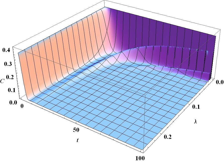
(a)

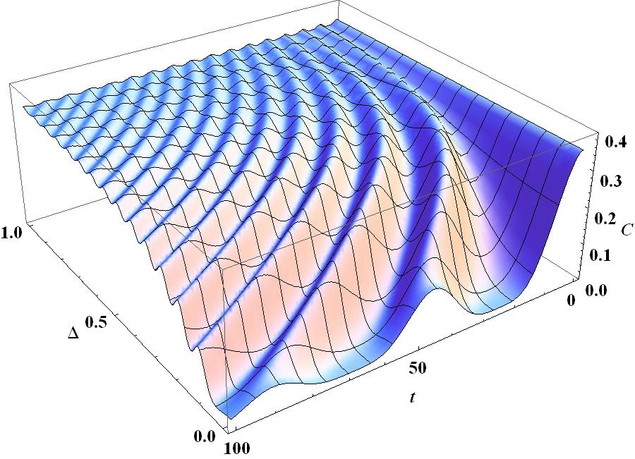
(b)

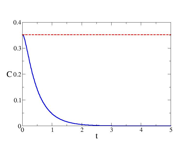
(c)

Figure 1: Entanglement evolution of two qubits with the initial density matrix (29) subject to amplitude damping noises. We plot the concurrence for (a) different $\lambda$ at fixed detuning $\Delta=0.01\gamma$ and (b) different $\Delta$ at fixed coupling bandwidth $\lambda=0.01\gamma$. In (c) the solid curve depicts the entanglement evolution for large coupling bandwidth $\lambda=10.0\gamma$ (with $\Delta=0.01\gamma$), and the dashed curve for large detuning $\Delta=10.0\gamma$ (with $\lambda=0.01\gamma$); note that for clarity, the time axis in (c) has a smaller range than those in (a), (b). The axes $\lambda$ in (a) and $\Delta$ in (b) are in units of $\gamma$, while the time axes in all plots are in units of $1/\gamma$.

Fig. 1 displays our results for the entanglement evolution of two qubits with the initial density matrix

$$\rho(0)=\frac{1}{3}\left(\begin{array}[]{cccc}\frac{1}{3}&0&0&0\\ 0&1&1&0\\ 0&1&1&0\\ 0&0&0&\frac{2}{3}\end{array}\right)\,,$$ (29)

which is an entangled mixed state. In Fig. 1(a) we plot the concurrence evolution at fixed detuning $\Delta=0.01\gamma$ for different values of $\lambda$. It is seen clearly that the crossover from oscillatory behavior to monotonic decay occurs when the coupling bandwidth changes from small to large values. In Fig. 1(b) the concurrence evolution is plotted at fixed coupling bandwidth $\lambda=0.01\gamma$ for different values of detuning $\Delta$. One can observe that the entanglement evolution changes from damped oscillatory behavior to barely damped one as the detuning varies from small to large values. Since entanglement preservation is a key issue in quantum information sciences, it is of great interest to analyze in detail how such transitions arise. Let us first attempt with simple, qualitative reasoning.

For the results in Fig. 1(a), when the coupling bandwidth is small ($\lambda\ll\gamma$), it corresponds to the limit with each qubit coupled to almost just one single oscillator mode. The entanglement dynamics is thus non-dissipative since the entanglement can transfer back and forth between the qubits and the oscillator modes involved [20, 21]. In other words, in the limit of long noise coherence time (ie. large $\lambda^{-1}$) the environment memory can reconstruct the qubit entanglement, so that the concurrence displays an oscillation that is hardly damped. In the other limit of large coupling bandwidth ($\lambda\gtrsim\gamma$; see the solid line in Fig. 1(c)), the qubits are coupled to a wide spectrum of oscillator modes. Thus the environment memory time becomes exceedingly short, so that the entanglement dynamics becomes Markovian and the concurrence decays to zero monotonically. In the intermediate regime, due to the finite environment memory time, concurrence oscillation is damped but approaches zero in a non-monotonic manner. Since entanglement oscillation is an indication for non-Markovian dynamics [8, 14, 9], the crossover associated with the coupling bandwidth can also be regarded as one between the limits of Markovian and “extremely” non-Markovian dynamics.

For the results in Fig. 1(b), we note that for large detuning ($\Delta\gtrsim\gamma$; see also the dashed line in Fig. 1(c)) the qubits can only couple weakly to the environment noises. The concurrence is thus barely damped in this limit. With decreasing detuning, the environment noise can couple more and more effectively to the qubits, which results in stronger and stronger damping in the concurrence evolution. Therefore, the crossover from undamped to damped oscillatory entanglement dynamics that we are seeing in Fig. 1(b) is connected with the transition between the weak and strong coupling limits in the qubit-environment interaction.

In order to substantiate the arguments above, let us now turn to more quantitative, detailed analysis for the behavior of $p(t)$ based on (15).

1. Small coupling bandwidth

In the limit of small $\lambda$, suppose $\lambda\ll\Delta\ll\gamma$, one can find from (16) that

$$d\simeq i\sqrt{2\gamma\lambda+\Delta^{2}}\equiv i\,\omega_{d}\,.$$ (30)

Hence it follows from (15)

$$p(t)\simeq e^{i\frac{\Delta}{2}t}\left[\cos\left(\frac{\omega_{d}}{2}t\right)-\frac{i\Delta}{\omega_{d}}\sin\left(\frac{\omega_{d}}{2}t\right)\right]\,,$$ (31)

which oscillates in time with no damping. This gives rise to the undamped concurrence oscillations, which are manifestations of non-dissipative dynamics. Note that this regime is small in Fig. 1(a); it can be seen more clearly in Fig. 1(b). For larger bandwidths $\Delta\ll\lambda\ll\gamma$, one can obtain from (16)

$$d\simeq i\sqrt{2\gamma\lambda}\,,$$ (32)

and thus (15) would yield

$$p(t)\simeq e^{-\frac{\lambda t}{2}}\cos\left(\sqrt{\frac{\gamma\lambda}{2}}t\right)\,.$$ (33)

We see that $p(t)$ is now oscillating with frequency $\sqrt{\gamma\lambda/2}$ with a damping time $\sim\lambda^{-1}$. Therefore for $\lambda\ll\gamma$, there can be many oscillations within the damping time; one would thus find weakly damped concurrence oscillations in this regime.

It should be noted that in the limit under consideration, if the detuning is large, such that $\Delta\gg\gamma\gg\lambda$, then we have from (16)

$$d\simeq\lambda-i\Delta\,.$$ (34)

It then follows readily from (15)

$$p(t)\simeq 1\,.$$ (35)

The concurrence thus remains a constant throughout the time evolution; see the dashed curve in Fig. 1(c). As explained above, this is because the detuning is so large here that the qubit-environment coupling becomes no longer effective. The qubit dynamics thus becomes entirely immune to the environment noise.

2. Large coupling bandwidth

In the limit of large coupling bandwidth, suppose $\lambda\gg\gamma\gg\Delta$, it follows from (16) that

$$d\simeq\lambda-\gamma-i\Delta\,.$$ (36)

One can thus obtain from (15)

$$p(t)\simeq e^{-\frac{\gamma}{2}t}\,,$$ (37)

which is typical Markovian behavior. The concurrence evolution is therefore strongly damped in this regime and decays to zero monotonically (see the solid curve in Fig. 1(c)). Note that in arriving at (37) the detuning has been taken to be small, ie. $\Delta\ll\lambda,\gamma$. If we have large detuning, so that $\lambda\gg\Delta\gg\gamma$ or $\Delta\gg\lambda\gg\gamma$, it is easy to show that one would get $p(t)\simeq 1$ in both cases. The concurrence thus becomes stationary due to the ineffective coupling at large detunings.

3. Spectral function

To further justify the foregoing analysis in 1. and 2., it is also instructive to examine the spectral function $J(\omega)$ in the corresponding limits. In the limit of small coupling bandwidth, one has from (14)

$$\lim_{\lambda\rightarrow 0}J(\omega)=\frac{\gamma\lambda}{2}\delta(\omega-\omega_{0}+\Delta)\,,$$ (38)

which signifies that, as noted above, each qubit is coupled to a single oscillator mode with frequency $\omega_{0}-\Delta$. As a consequence, a non-dissipative, oscillatory concurrence evolution follows. In fact, making use of (38) in (13), and then solving $p(t)$ from (11), one can recover (31) accordingly. In the limit of large coupling bandwidth, one finds similarly from (14)

$$\lim_{\lambda\rightarrow\infty}J(\omega)=\frac{\gamma}{2\pi}\,.$$ (39)

Therefore, we have a white noise spectrum for the qubit-environment coupling in this limit. The entanglement dynamics thus becomes Markovian and the concurrence decreases to zero monotonically. Again, using (39) in (13), one can regain (37) easily from (11). In the intermediate regime between the two extremes, the concurrence displays damped oscillations, where the oscillations are manifestations of the finite environment memory times due to non-zero coupling bandwidths.

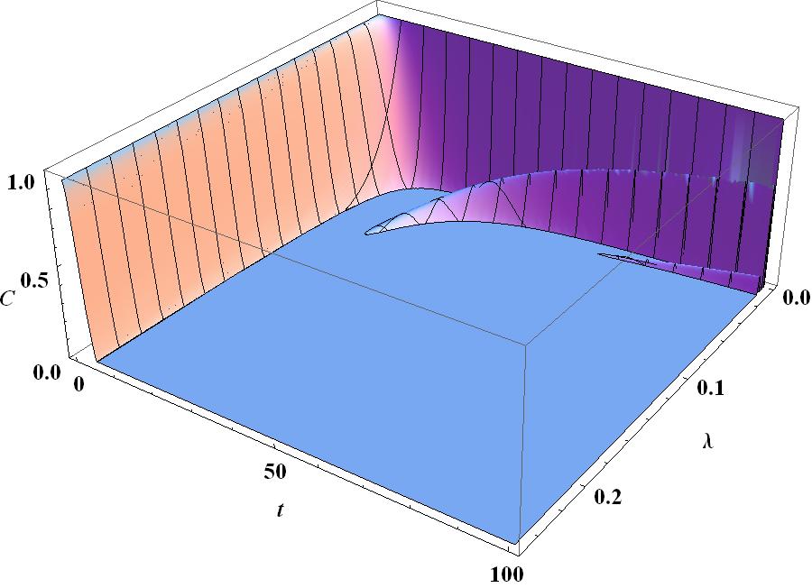
(a)

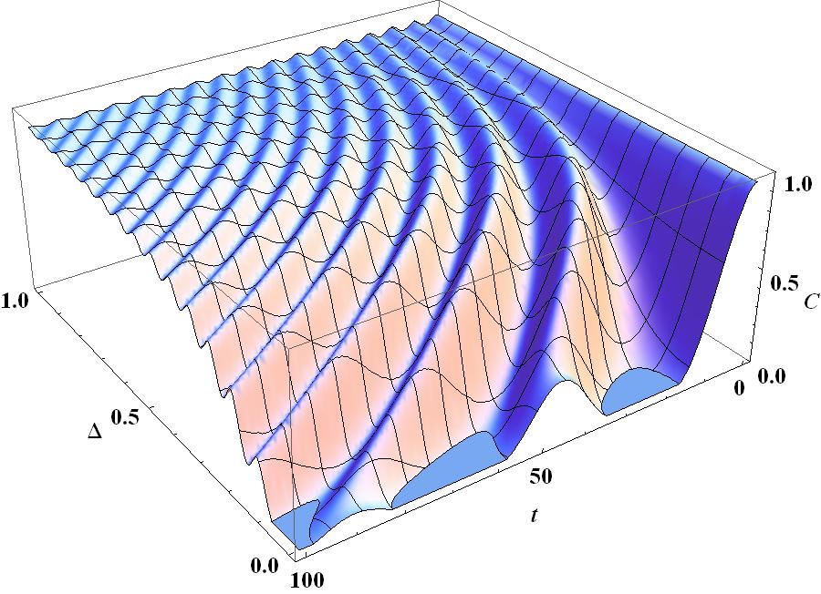
(b)

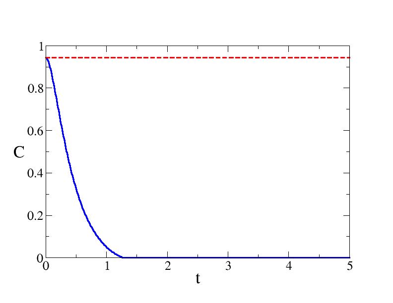
(c)

Figure 2: Same as Fig. 1 but for the initial density matrix (44). The flat regions at the base planes of (a) and (b) are signatures of entanglement sudden death.

As another example, we consider an entangled pure initial state which has the density matrix

$$\rho(0)=\frac{1}{3}\left(\begin{array}[]{cccc}2&0&0&\sqrt{2}\\ 0&0&0&0\\ 0&0&0&0\\ \sqrt{2}&0&0&1\end{array}\right)\,.$$ (44)

The results for the calculation are shown in Fig. 2. Although there are now regions with entanglement sudden death (and rebirth), our explanations above for the concurrence oscillation/damping in Fig. 1 can be carried over.

IV. Phase damping

A. Single-qubit dynamics

Let us now turn to another class of qubit-environment interaction that couples longitudinally to the (pseudo)spin of the qubit. The environment noise would therefore not cause any energy relaxation in the qubit, but randomize the relative phase between the qubit levels. In the single-qubit Hamiltonian (1), this coupling can be modeled with the following qubit-environment interaction [22]

$$H_{I}=\sum_{k}\sigma_{z}\left(g_{k}b_{k}^{\dagger}+g_{k}^{*}b_{k}\right)\,,$$ (45)

where, as previously, $g_{k}$ are the coupling constants. Unlike (5), here $H_{I}$ commutes with the bare qubit Hamiltonian $(\omega_{0}/2)\sigma_{z}$, and thus would not induce any population transfer between the qubit levels $|+\rangle$ and $|-\rangle$. The coupling (45) would instead act like a fluctuating magnetic field along $z$-direction that can randomize the phase of the qubit [22]. This qubit-environment coupling is thus often referred to as the phase damping channel [1].

For the interaction Hamiltonian (45), one can work out the time evolution of the qubit explicitly [22]. It is then not difficult to find the corresponding single-qubit operation elements. Suppose the environment is initially in the vacuum state, in the usual basis $\{|+\rangle,|-\rangle\}$ one can find

$$E_{1}=\left(\begin{array}[]{cc}p&0\\ 0&1\end{array}\right)\,,\quad E_{2}=\left(\begin{array}[]{cc}q&0\\ 0&0\end{array}\right)\,,$$ (50)

where, as before, $q\equiv\sqrt{1-|p|^{2}}$. Here we have

$$p(t)=\exp\{\Gamma(t)\}$$ (51)

with

$$\Gamma(t)\equiv-2\sum_{k}|g_{k}|^{2}\int_{0}^{t}d\tau\int_{0}^{t}d\tau^{\prime}e^{-i\omega_{k}(\tau-\tau^{\prime})}$$ (52)

a real negative function of time. As in the case of amplitude damping, we can rewrite $\Gamma(t)$ of (52) in terms of the noise correlation function $f(t)$ and the spectral function $J(\omega)$ using (13); we get

$$\Gamma(t) = -2\int_{0}^{t}d\tau\int_{0}^{t}d\tau^{\prime}f(\tau-\tau^{\prime})e^{-i\omega_{0}(\tau-\tau^{\prime})}$$ (53)

$$= -2\int_{0}^{t}d\tau\int_{0}^{t}d\tau^{\prime}\int_{-\infty}^{\infty}\!\!d\omega\,J(\omega)e^{-i\omega(\tau-\tau^{\prime})}\,.$$

As previously, once a specific form for $J(\omega)$ is given, it is then possible to find the qubit dynamics accordingly.

Let us consider again the Lorentzian spectral function (14). Note, however, that since the interaction (45) would not cause any transition between the qubit levels $|+\rangle$ and $|-\rangle$, the frequency $\omega_{0}$ no longer plays the role of the “resonant frequency”. One can thus redefine $\omega_{c}\equiv\omega_{0}-\Delta$ as the “central frequency” for the coupling (this follows from the form of the spectral function (14), which centers at $\omega=\omega_{c}$). Applying (14) in (53), one can obtain

$$\Gamma(t) = -2\gamma\lambda\Bigg{\{}\frac{\lambda}{\lambda^{2}+\omega_{c}^{2}}t$$ (54)

$$-\frac{1}{(\lambda^{2}+\omega_{c}^{2})^{2}}\Big{[}(\lambda^{2}-\omega_{c}^{2})\left(1-e^{-\lambda t}\cos(\omega_{c}t)\right)$$

$$+2\lambda\omega_{c}e^{-\lambda t}\sin(\omega_{c}t)\Big{]}\Bigg{\}}\,.$$

It is interesting to note that for non-zero $\omega_{c}$, $\Gamma(t)$ (and hence $p(t)$) can oscillate in time. The qubit decoherence can consequently occur non-monotonically. In the case of two qubits, this can lead to entanglement oscillations, as we shall now show.

B. Two-qubit dynamics

For two independent qubits $A$, $B$ subject to uncorrelated local phase noises, again, we resort to the prescription outlined in Sec. II.. Using (50) in (3), one can derive the two-qubit operation elements in the phase damping channel. Substituting the results into (4), one can then obtain the time evolution of the the matrix elements for the two-qubit reduced density matrix (in the basis $\{|++\rangle,|+-\rangle,|-+\rangle,|--\rangle\}$)

$$\rho_{ii}(t) = \rho_{ii}(0)\,,\quad\mbox{$i=1\sim 4$.}$$

$$\rho_{12}(t) = p_{B}\,\rho_{12}(0)\,,$$

$$\rho_{13}(t) = p_{A}\,\rho_{13}(0)\,,$$

$$\rho_{14}(t) = p_{A}\,p_{B}\,\rho_{14}(0)\,,$$

$$\rho_{23}(t) = p_{A}\,p_{B}\,\rho_{23}(0)\,,$$

$$\rho_{24}(t) = p_{A}\,\rho_{24}(0)\,,$$

$$\rho_{34}(t) = p_{B}\,\rho_{34}(0)\,,$$ (55)

where $p_{\alpha}$ are the expressions for qubit $\alpha=A,B$ in accordance with (51) and (54) (with appropriate qubit labels added). Note that here we have made use of the fact that $p_{A,B}(t)$ are real functions of time. From (55) we see that, as noted previously the phase noise does not affect the qubit occupations since the diagonal elements of the reduced density matrix remain unchanged. However, it diminishes the coherence of the density matrix by corroding the off-diagonal elements of the reduced density matrix.

In order to examine the entanglement dynamics ensued from (55), again we shall consider initial density matrices of the X-form (23). The concurrence of the qubits can then be calculated using (51), (54) together with (55) in (24). As previously, we shall consider symmetric configurations where the two qubits are identical (so that they have the same level separation $\omega_{0}$ and the same decay rate $\gamma_{A}=\gamma_{B}=\gamma$) and the phase noises acting on them have the same characteristics, namely $\lambda_{A}=\lambda_{B}=\lambda$, $\omega_{c}^{A}=\omega_{c}^{B}=\omega_{c}$, and consequently $p_{A}=p_{B}=p$ in (55).

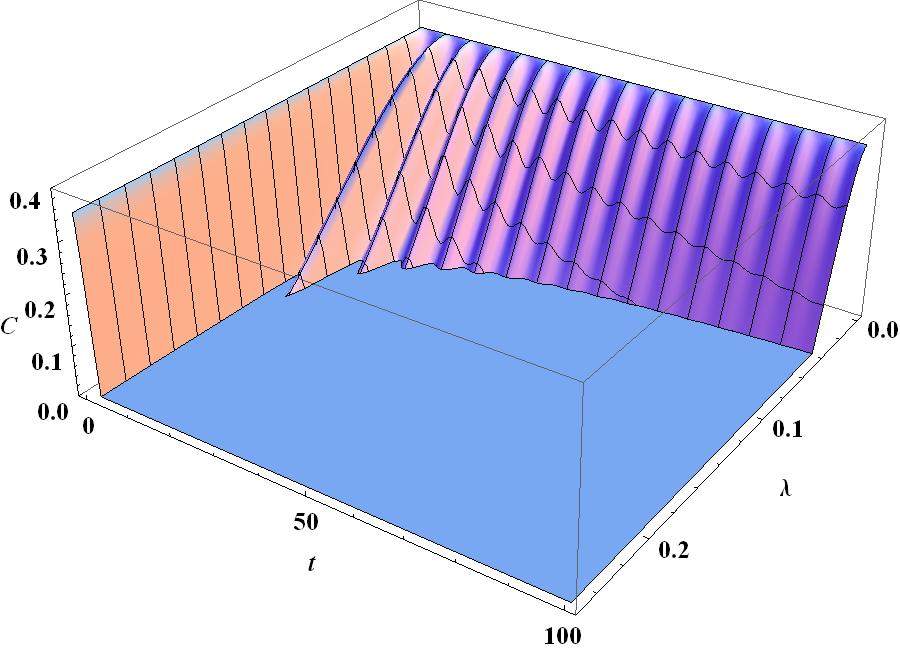
(a)

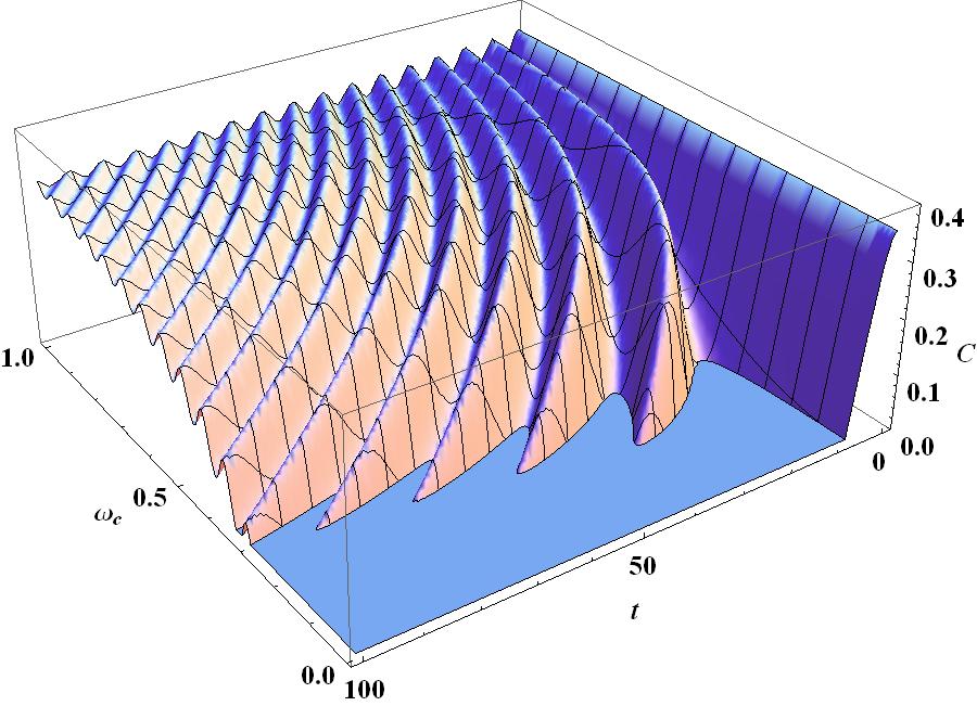
(b)

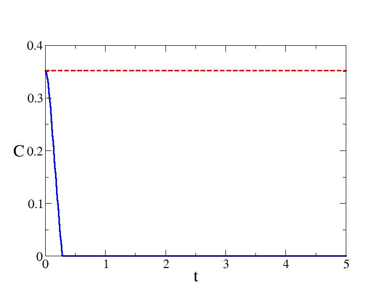
(c)

Figure 3: Entanglement evolution of two qubits with the initial density matrix (29) subject to phase damping noises. Here we plot the concurrence for (a) different $\lambda$ at fixed central frequency $\omega_{c}=1.0\gamma$ and (b) different $\omega_{c}$ at fixed coupling bandwidth $\lambda=0.01\gamma$. In (c) the solid curve illustrates the entanglement evolution for large coupling bandwidth $\lambda=10.0\gamma$ (with $\omega_{c}=1.0\gamma$), and the dashed curve for large central frequency $\omega_{c}=10.0\gamma$ (with $\lambda=0.01\gamma$). For clarity, we plot in (c) a smaller range of time than in (a), (b). The units for the axes are the same as in Fig. 1. The flat areas at the base planes in (a) and (b) indicate regions with entanglement sudden death.

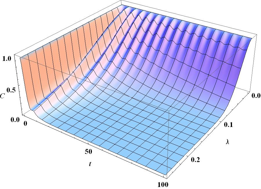
(a)

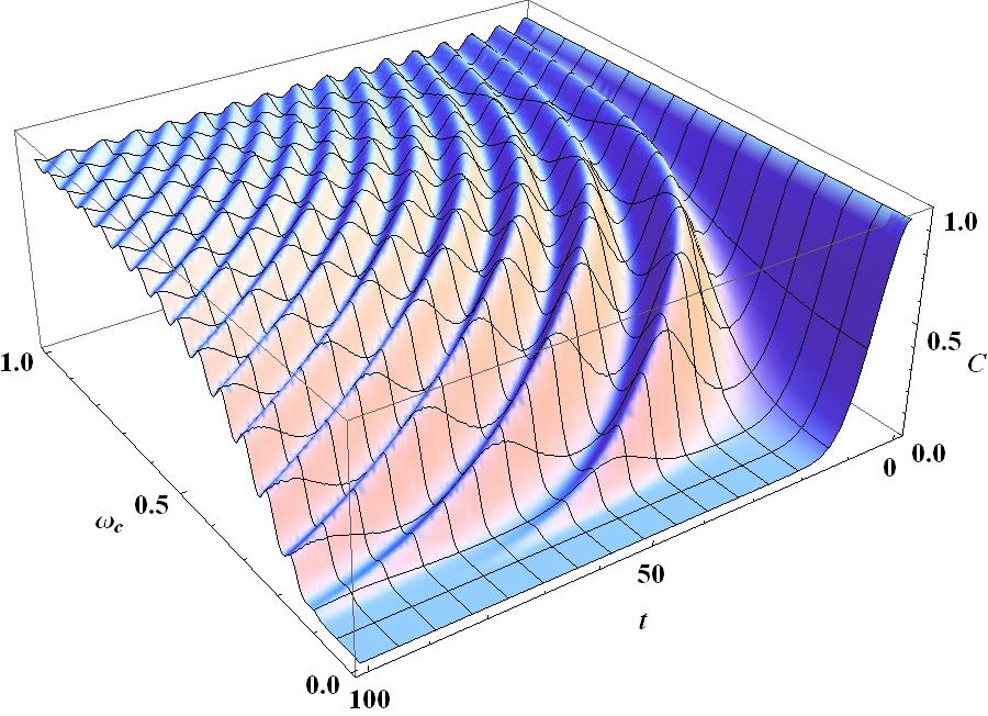
(b)

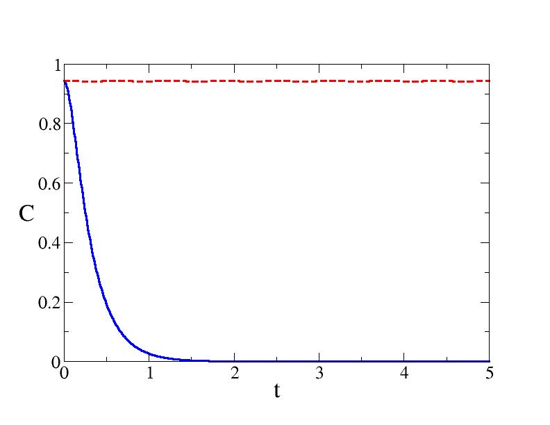
(c)

Figure 4: Same as Fig. 3 but for the initial density matrix (44).

Fig. 3 illustrates our results for the entanglement evolution of two qubits with the initial density matrix (29). In Fig. 3(a) we plot the concurrence evolution at fixed central frequency $\omega_{c}=1.0\gamma$ for different coupling bandwidths $\lambda$. When the coupling bandwidth varies from small to large values, crossover from oscillatory behavior to monotonic decay in the concurrence evolution can be seen clearly. In Fig. 3(b) the concurrence evolution is plotted at fixed coupling bandwidth $\lambda=0.01\gamma$ for different central frequencies $\omega_{c}$. One can observe that the entanglement evolution changes from monotonically decaying behavior to barely damped oscillations as $\omega_{c}$ varies from small to large values. Another set of results for the entanglement dynamics under phase damping noise is illustrated in Fig. 4, where we consider the initial density matrix (44). Again, similar crossovers between different regimes are clearly visible.

Qualitatively, the results in Figs. 3 and 4 can be understood in the same manner as presented in Sec. III. for the entanglement evolution under amplitude damping noise. For instance, in both Figs. 3(a) and 4(a) the regime with small coupling bandwidths correspond to the limit with each qubit coupled to one single oscillator mode. The entanglement dynamics thus exhibits non-dissipative behavior, as entanglement swapping can take place between the pair of qubits and the two oscillator modes. The undamped entanglement oscillations in this regime are consequences of the long environment memory time $\lambda^{-1}$, which enables entanglement reconstructions in the qubits. For large coupling bandwidths, the wide spectrum of the qubit-environment coupling entails an extremely short environment memory time. Therefore, the Markovian entanglement dynamics emerges and the concurrence decays to zero monotonically (see the solid curves in Figs. 3(c) and 4(c)). For the intermediate regime, the finite coupling bandwidth implies non-vanishing environment memory time. The concurrence thus carries out damped oscillations, in which the oscillatory part reflects the memory effect that survives the phase damping noise.

As pointed out earlier in the present section, the central frequency $\omega_{c}$ is the peak frequency for the qubit-environment coupling. Therefore, at large $\omega_{c}$ the qubits are coupled to the phase noise only very weakly. This is why in both Figs. 3(b) and 4(b) the concurrence is barely damped at large $\omega_{c}$ (see also the dashed curves in Figs. 3(c) and 4(c)). With decreasing $\omega_{c}$, as the noise can couple more and more effectively to the qubits, damping in the concurrence evolution gradually sets in. Eventually, in the limit of small $\omega_{c}$, the entanglement oscillation disappears and the concurrence drops to zero monotonically.

As in Sec. III., more quantitative analysis for the results here can be achieved by looking into the behavior of $p(t)$ according to (51) and (54) in the limits of small and large coupling bandwidths. It should be noted, however, that unlike amplitude damping noise, here the regimes of small and large coupling bandwidths are determined from the relative magnitude between $\lambda$ and $\omega_{c}$ (instead of the qubit decay rate $\gamma$). This is because under the action of phase damping noise, the qubit populations would not change. Thus the time scale $\gamma$ becomes inessential to the non-Markovian dynamics of the qubit (see later). Instead, it is the central frequency $\omega_{c}$ that comes into play (which is clear from the explicit form of $\Gamma(t)$ in (54)). Therefore, for phase damping noise although the central frequency $\omega_{c}$ plays a role similar to the detuning $\Delta$ in amplitude damping noise, the concurrence oscillation depends more sensitively on $\omega_{c}$ (compare Figs. 1(b) with 3(b), and Figs. 2(b) with 4(b), especially for regions with small $\Delta$ and $\omega_{c}$). With the above observations, let us now examine $p(t)$ for small and large coupling bandwidths using (51) and (54).

1. Small coupling bandwidth

For narrow coupling bandwidths $\lambda\ll\omega_{c}$, we find from (54) that

$$\Gamma(t)\simeq-\frac{2\gamma\lambda}{\omega_{c}^{2}}\left[1+\lambda t-e^{-\lambda t}\cos(\omega_{c}t)\right]\,.$$ (56)

Therefore for times $t\ll\lambda^{-1}$, $p(t)=\exp\{\Gamma(t)\}$ oscillates with negligible damping and the concurrence dynamics exhibits non-dissipative characteristics. This can again be anticipated from the spectral function $J(\omega)$, which reduces to the form for single mode coupling in this limit (see (38)). Indeed, using the spectral function (38) in (53), one can derive an expression for $\Gamma(t)$ which has exactly the same form as (56) except with $\lambda t=0$ (ie. being totally non-dissipative). For $\lambda t\sim 1$, however, we see from (56) that damping begins to set in. As a result, the oscillating cosine term in (56), which represents the environment memory effect, is attenuated and a damped concurrence oscillation thus follows. At long times $t\gg\lambda^{-1}$, one can infer from (56) that $p(t)$ eventually drops to zero exponentially, thus also the concurrence (save the complications due to entanglement sudden death, such as in Fig. 3).

Note that in the present limit, if the central frequency is so large that $\omega_{c}\gg\gamma,\lambda$, it follows from (56) that $\Gamma(t)$ would become vanishing. In this case we have $p(t)\simeq 1$ and the entanglement becomes stationary, as the qubit is completely decoupled from the environment in this limit. This can be seen from the dashed curves in Figs. 3(c) and 4(c).

2. Large coupling bandwidth

For large coupling bandwidths $\lambda\gg\omega_{c}$, it follows from (54) that

$$\Gamma(t)\simeq-2\gamma\left(t-\frac{1-e^{-\lambda t}\cos(\omega_{c}t)}{\lambda}\right)\,.$$ (57)

Since $\lambda$ is now large, the damping time (or environment memory time) $\lambda^{-1}$ is short. Within the damping time, the oscillatory cosine term in (57) cannot even complete one period since $\omega_{c}\lambda^{-1}\ll 1$ here; the environment memory is therefore washed away quickly. For times $t\gg\lambda^{-1}$, we get from (57) that

$$p(t)=\exp\{\Gamma(t)\}\simeq e^{-2\gamma t}\,,$$ (58)

which manifests the Markovian nature of this limit. As a consequence, the concurrence becomes strongly damped and exhibits Markovian behavior [11]. As previously, we can further corroborate the argument above by considering the spectral function $J(\omega)$ in the present limit; the white noise spectrum (see Eq. (39)) is again responsible for the Markovian entanglement dynamics in this limit. As a check, one can use (39) in (53), which would yield (58) immediately.

V. Discussions and Conclusions

In summary, based on exactly solvable models, we have studied the entanglement dynamics of a pair of non-interacting qubits that are separately coupled to their local environments. In particular, we examine in detail the crossover between the limits of dissipative and non-dissipative entanglement dynamics that are manifested in the damped/undamped concurrence oscillations. We show that this crossover is connected with the bandwidth of the qubit-environment coupling. We have also studied the crossover between the limits of strong and weak couplings, which is controlled by the detuning of the qubit-environment interaction. Both categories of crossovers have been considered for two types of environment noises, the amplitude damping channel and the phase damping channel, and physical pictures for the results have been provided.

Although we have illustrated our results only for two specific initial density matrices (29) and (44), our conclusions are indeed fairly general. For instance, suppose only one of the qubits is coupled to the environment, it is easy to derive from our formulas that the concurrence evolution for any pure initial state would follow the factorization law [23, 9]

$$C(t)=|p(t)|C(0)\,,$$ (59)

where $p(t)$ is given by (15) and (51), respectively, for amplitude and phase damping noises. Since for maximally entangled pure initial states $C(0)=1$, it follows that $p(t)$ completely determines the concurrence evolution of the the maximally entangled state for this noisy channel. Therefore, according to (59), for any pure initial state the concurrence evolves according to the action of the noisy channel over the maximally entangled state [23]. The oscillation/damping of $p(t)$ in different regimes would thus exhibit also in the concurrence evolution for general pure initial states. Similar results exist also for certain class of mixed initial states when both qubits are subject to local noises [9].

An issue that we did not address in this paper is the interplay between amplitude noise and phase noise. For Markovian entanglement dynamics, Yu and Eberly had demonstrated that the combination of phase damping and amplitude damping noises can give rise to non-additive entanglement dissipation [24]. For the non-Markovian case, it is certainly of interest to investigate whether additional effects would emerge when both phase and amplitude noises are present. Also, in our analysis of the entanglement evolution, we did not examine the detailed dynamics close to entanglement sudden death. We wish to take up these issues in future works.

References

- 1. See, for example, M. A. Nielsen and I. L. Chuang, Quantum Computation and Quantum Information (Cambridge University Press, Cambridge, 2000) and J. Preskill, Lecture Notes on Quantum Information and Quantum Computation, available at http://www.theory.caltech.edu/people/preskill/ph229.
- 2. See, for instance, D. Bouwmeester, A. Ekert, and A. Zeilinger (Eds.), The Physics of Quantum Information (Springer, Berlin, 2000).
- 3. See, for example, F. Mintert, A. R. R. Carvalho, M. Kuś, and A. Buchleitner, Phys. Rep. 415, 207 (2005), R. Horodecki, P. Horodecki, M. Horodecki, and K. Horodecki, Rev. Mod. Phys. 81, 865 (2009), O. Gühne and G. Tóth, Phys. Rep. 474, 1 (2009) and references therein.
- 4. See T. Yu and J. H. Eberly, Science 323, 598 (2009) and references therein.
- 5. T. Yu and J. H. Eberly, Phys. Rev. Lett. 93, 140404 (2004).
- 6. M. P. Almeida et al., Science 316, 579 (2007).
- 7. J. Laurat et al., Phys. Rev. Lett. 99, 180504 (2007).
- 8. B. Bellomo, R. Lo Franco, and G. Compagno, Phys. Rev. Lett. 99, 160502 (2007).
- 9. J. G. Li, J. Zou, and B. Shao, Phys. Rev. A 82, 042318 (2010).
- 10. J.-S. Xu et al., Phys. Rev. Lett. 104, 100502 (2010).
- 11. T. Yu and J. H. Eberly, Opt. Comm. 283, 676 (2010).
- 12. M. M. Wolf et al., Phys. Rev. Lett. 101, 150402 (2008).
- 13. H.-P. Breuer, E.-M. Laine, and J. Piilo, Phys. Rev. Lett. 103, 210401 (2009).
- 14. Á. Rivas, S. F. Huelga, and M. B. Plenio, Phys. Rev. Lett. 105, 050403 (2010).
- 15. K. Kraus, States, Effects, and Operations: Fundamental Notions of Quantum Theory (Springer-Verlag, Berlin, 1983).
- 16. H.-P. Breuer and F. Petruccione, The Theory of Open Quantum Systems (Oxford University Press, Oxford, 2002).
- 17. B. M. Garraway, Phys. Rev. A 55, 2290 (1997).
- 18. W. K. Wootters, Phys. Rev. Lett. 80, 2245 (1998).
- 19. T. Yu and J. H. Eberly, Quant. Inf. Comput. 7, 459 (2007).
- 20. M. Yönaç, T. Yu, and J. H. Eberly, J. Phys. B: At. Mol. Opt. Phys. 39, S621 (2006).
- 21. M. Yönaç,T. Yu, and J. H. Eberly, J. Phys. B: At. Mol. Opt. Phys. 40, S45 (2007).
- 22. G. M. Palma, K.-A. Suominen, and A. K. Ekert, Proc. R. Soc. Lon. A452, 567 (1996).
- 23. T. Konard et al., Nat. Phys. 4, 99 (2008).
- 24. T. Yu and J. H. Eberly, Phys. Rev. Lett. 97, 140403 (2006).