Planar Pixelations and Image Recognition

Abstract.

Any subset of the plane can be approximated by a set of square pixels. This transition from a shape to its pixelation is rather brutal since it destroys geometric and topological information about the shape. Using a technique inspired by Morse Theory, we algorithmically produce a PL approximation of the original shape using only information from its pixelation. This approximation converges to the original shape in a very strong sense: as the size of the pixels goes to zero we can recover important geometric and topological invariants of the original shape such as Betti numbers, area, perimeter and curvature measures.

Introduction

A common problem in computational topology is to try to recover an object embedded in $\mathbb{R}^{n}$ when only some distorted version of it is known. Inspired by digital imaging we consider specifically the problem of a pixelated subset of the plane, which is to say that it has been replaced by a set of square pixels on a grid. Since it is common to represent images by a grid of small pixels, it seems intuitive that any object could be recovered from its pixelations. Indeed, when the resolution of an image is fine it is difficult to detect any difference from the original using only the human eye, and we may expect to be able to recover even deep geometric invariants.lated subset of the plane, which is to say that it has been replaced by a set of square pixels on a grid. Since it is common to represent images by a grid of small pixels, it seems intuitive that any object could be recovered from its pixelations. Indeed, when the resolution of an image is fine it is difficult to detect any difference from the original using only the human eye, and we may expect to be able to recover even deep geometric invariants.

A pixelation associated to a subset of a plane is simply the set of all pixels in a grid of a certain size which touch that subset (see Figure 1). By changing the size of the grid, we can view pixelations of the object with finer and courser resolutions. We call the pixelation associated to a set $S\subset\mathbb{R}^{2}$ created from a grid of side-length $\varepsilon$ $P_{\varepsilon}(S)$, or the $\varepsilon$-pixelation of $S$ (see Definition 1.1). The variable $\varepsilon$ is called the resolution of the pixelation.

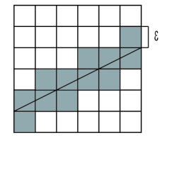
Figure 1. An example pixelation of a line with slope $\frac{1}{2}$

For small resolutions these pixelations seem to resemble the original shape. However, we need a precise notion of what it means to resemble the original object. At the very least it seems that the important topological and geometric invariants of the pixelation will be close to the corresponding variants of the original set. Even when viewing simple examples, we can quickly see that not all invariants will converge for small resolutions. Most obviously, the total curvature of $P_{\varepsilon}(S)$ will tend to increase to infinity, since the pixelation contains many corners. Similarly length of the boundary may not converge. To see this consider the line segment from $(0,0)$ to $(1,1)$. The length of the line is $\sqrt{2}$, but each of its pixelations will have a boundary whose length is close to $4$.

We see that pixelations do destroy various geometric invariants. However, it may be that convergence of these invariants is too much to ask for. A much simpler request is for the pixelation to eventually converge in Euler characteristic. Unfortunately not even this is guaranteed. Some pixelations will contain fake cycles which do not correspond to any cycle of the original set (indeed arbitrarily many may appear even if the original set was contractible). Worse yet, these fake cycles may not disappear for small resolutions. Section A has further information on this phenomenon, but for now it is sufficient to consider the example of a line of slope $1$ and a line of slope $\frac{2}{3}$ (which is shown in Figure 2). The $\varepsilon$-pixelations have certain scale invariance properties which guarantee that a fake cycle will always appear, even for very small $\varepsilon$.

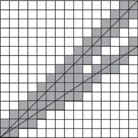
Figure 2. The pixelation of the angle $A\left(1,\frac{2}{3}\right)$ contains two holes.

We see that the process of pixelation can destroy a great deal of mathematical information of the set. However, to the eye, the pixelation can look very close to the original set. Therefore it seems that it should be possible to use only the pixelation to reconstruct the original set. In this paper we will create an explicit algorithm which can reconstruct a PL set $S$ from only its pixelations. However, to motivate this algorithm and to generate the theorems needed to show that this algorithm works, we will need to examine simpler examples of pixelations.

In Section 2 we deal with pixelations of the graphs of $C^{2}$ functions. Theorem 2.2, an analogue of the intermediate value theorem, tells us that these pixelations must be contractible. Therefore we do not have to worry at this stage about fake cycles. To approximate the graph of a function we attempt to use a secant line approximation. This is done by connecting points within the pixelation of the function to create a PL approximation. However, additionally error will be generated from the fact that our sample points are being selected not from the graph of function, but merely near to the graph.

Theorem 2.6 gives us bounds on the error between a secant line of our function and the approximate secant line from the pixelation. Note that these bounds depend both on the resolution $\varepsilon$ and the width of the secant line. We want to choose our PL approximation in a strict algorithmic way such that these errors vanish. To do this we use the notion of a spread function.

A spread function is simply a function $\sigma:\mathbb{R}^{+}\to\mathbb{Z}^{+}$ such that the following conditions hold:

$$\lim_{\varepsilon\searrow 0}\sigma(\varepsilon)=\infty,\;\;\lim_{\varepsilon\searrow 0}\varepsilon\sigma(\varepsilon)=0.$$

The spread function tells how wide the secant lines in our approximations should be in terms of the resolution of the pixelation. That is, since a pixel is defined to be $\varepsilon$ wide, the secant lines should be arranged to be about $\varepsilon\sigma(\varepsilon)$ wide. Theorem 2.11 shows that the two conditions of the spread $\sigma$ guarantee Sobolev $W^{1,p}$ convergence of the secant line approximation.

In Section 3 we generalize the approximation technique to handle elementary regions, which are defined to be regions which line in between the graphs of two $C^{2}$ functions (note that the graph of a $C^{2}$ function is just a special case of an elementary region). In this case we also cannot have fake cycles. We can easily generalize the secant line approximation of functions to elementary regions by approximating the top and bottom regions of the elementary region. It is then simple to show that we maintain the previous Sobolev $W^{1,p}$ convergence on the boundary of the approximation.

Here the notion of a spread becomes very useful. By restricting the spread function $\sigma$, we can dramatically improve the convergence of the approximation. Indeed if require that

$$\lim_{\varepsilon\searrow 0}\varepsilon(\sigma(\varepsilon))^{2}=\infty,$$

so that $\sigma$ increases very quickly, but still does not increase faster than $\varepsilon$ decreases, we can recover the total curvature of the boundary of the elementary region. This is shown in Propositions 3.4, 3.6 and Corollary 3.7 for sets of increasing generality. However each of these sets is defined as the region between the graphs of two functions.

At this point although we have created an algorithm which strongly approximates an elementary regions, but we have completely ignored simple sets such as the union of two intersecting lines. Such a set is potentially difficult to approximate, since its pixelation may have more cycles than the original set. In Section 4 we tackle the problem of homotopy type as it relates to the pixelations of $PL$ sets.

Corollary 4.2 of Theorem 4.1 shows that eventually there is a bijective correspondence between the connected components of the pixelation and the connected components of the original set $S$. A cycle in a (reasonably behaved) planar set corresponds to a hole, i.e., a bounded connected component of the complement of the set. We can again use Theorem 4.1 to show that every hole of the original set $S$ will eventually correspond to a hole of the pixelation. Therefore any defect in homotopy type is caused by the addition of holes in the process of pixelation. This means that to ensure convergence in homotopy type, we need only to delete the extra holes using only information from the pixelation.

An intuitive way to distinguish fake holes from real holes is to note that any real hole must take up an actual area in the plane. However, fake holes tend to be composed of a relatively small number of really small pixels. Therefore for small resolutions $\varepsilon$ the fake cycles will have small areas. Appealing as it may sound, this idea is difficult to implement rigorously because we do not have an accurate way of defining what “small area” means. We rely instead on a more robust approach inspired from Morse theory.

We consider the linear function on the Cartesian plane that associates to each point its $x$-coordinate. For simplicity we assume that its restriction $\ell_{S}$ to our PL set $S$ is a stratified Morse function in the sense of Goresky-MacPherson, [9]. In our case this simply means that no two vertices of our $PL$ set $S$ lie on the same vertical line.

The topology of the level sets of $\ell_{S}$ is determined by the counting function $\boldsymbol{n}$

$$\boldsymbol{n}(x):=\mbox{the number of components of $\ell_{S}^{-1}(x)$}.$$

A pixelated version of $\boldsymbol{n}$ is the function $\boldsymbol{n}_{\varepsilon}$, where $\boldsymbol{n}_{\varepsilon}(x)$ is the number of connected components of the column of $P_{\varepsilon}(S)$ located at $x_{0}$. Note that for a cycle to appear in $S$, the function $\boldsymbol{n}_{S}$ must vary and likewise with the pixelation and $\boldsymbol{n}_{\varepsilon}$. Therefore determining whether a cycle in $P_{\varepsilon}(S)$ is a fake or really corresponds to a cycle in $S$ is a matter of determining how closely the function $\boldsymbol{n}_{\varepsilon}$ agrees with $\boldsymbol{n}_{S}$.

The Separation Theorem (Theorem 4.4) states that if $x$ is not a critical value of $\ell_{S}$ then $\boldsymbol{n}(x)=\boldsymbol{n}_{\varepsilon}(x)$ for all $\varepsilon$ sufficiently small. The critical values of $\ell_{S}$ correspond to points jumping points of $\boldsymbol{n}$, i.e., points of of discontinuity of $\boldsymbol{n}$. Using the Separation Theorem we prove several results indicating that the jumping points of $\boldsymbol{n}_{\varepsilon}$ and the jumping points of $\boldsymbol{n}_{S}$ are not far apart. This culminates in Proposition 4.10 which states that in the PL case jumping points of $\boldsymbol{n}_{S}$ must appear close to jumping points of $\boldsymbol{n}_{\varepsilon}$ and vice versa. Here “close” means within $\varepsilon\nu(S)$ where $\nu(S)$ is an integer determined by $S$ and called the noise range.

We ultimately want to classify an interval around every jumping point of $\boldsymbol{n}_{\varepsilon}$ as “noise.” To do this we must estimate the noise range $\nu(S)$, but this is determined by the original set $S$ and thus unknown given only the pixelation. However if we estimate the noise range using a spread $\sigma$ note that for small $\varepsilon$ we can guarantee that $\sigma(\varepsilon)>\nu(S)$ while $\varepsilon\sigma(\varepsilon)$ is small. Therefore if we classify an interval of width about $\varepsilon\sigma(\varepsilon)$ around each jumping point of $\boldsymbol{n}_{\varepsilon}$ as noise, we can ensure that eventually outside of the noise $\boldsymbol{n}_{\varepsilon}=\boldsymbol{n}_{S}$ while the noise region remains small.

The noise intervals are important since they are chosen to eventually contain all fake cycles of $P_{\varepsilon}(S)$ while taking up a vanishingly small portion of the real line. Therefore to approximate homotopy type within noise intervals we need only cover every cycle (since any cycle appearing will be a fake cycle). Since noise does not take up much of the plane, we do not need to be careful as to how we approximate within noise intervals, so we will do this by covering each connected component of the noise with the smallest rectangle which covers it.

Call the components of the complement of the noise intervals regular intervals. By the definition of noise, the regular intervals contain no jumping points of $\boldsymbol{n}_{\varepsilon}$. Therefore $\boldsymbol{n}_{\varepsilon}$ is continuous on the regular intervals, which implies that the parts of $P_{\varepsilon}(S)$ which lie over regular intervals look like strips that span the entire regular interval. Each strip can be interpreted as the pixelation of an elementary set and we have explained how to deal with such objects.

Putting together all these facts we obtain Algorithm 4.12 which associates to each $\varepsilon$-pixelation a $PL$ set. This algorithm works by using the function $\boldsymbol{n}_{\varepsilon}$ and the spread $\sigma$ to divide the pixelation into noise and regular intervals, and then approximates within each interval using the appropriate results. That is to say within noise intervals it covers each connected component with a rectangle and within regular intervals it connects the tops and bottoms of every $\sigma$-th column. An example of the result of this algorithm can be seen in Figure 3 and the Algorithm is restated in terms of a computer program in Appendix D.

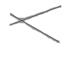
Figure 3. The result of Algorithm 4.12 as applied to the intersection of two red lines. Note that near the point of intersection the approximation resembles a rectangle, since this lies within a noise interval.

We wish to state that Algorithm 4.12 captures all the important geometric and topological invariants. To do this we use the language of normal cycles. These are $1$-currents with supports contained in the bundle of unit tangent vectors. Appendices B and C are included for readers unfamiliar with these objects. For purposes of this general discussion it suffices to mention that the normal cycle of a subanalytic subset $S$ of the plane is a piecewise $C^{1}$ closed curve in the unit tangent sphere bundle object which encodes geometric and topological information about of the set $S$ through integration of certain canonical 1-forms.

In general the normal cycle can be thought to be approximated by the collection of all unit outer normal vectors of the set. For example, the normal cycle of a bounded domain with $C^{2}$-boundary is the graph of the Gauss map of the boundary. The normal cycle of the square resembles Figure 4. Of course the normal cycle is actually a subset of the sphere bundle of the plane, not the plane itself. The fiber of the normal cycle over a point in the interior of an edge each point will consist of only a single outer normal vector. The fiber over a corner consists of an entire quarter-circle (all possible outer normal vectors for the corner). Therefore the length of the normal cycle will be the perimeter of the square plus $2\pi$, or the perimeter of the square plus its total curvature.

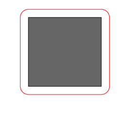
Figure 4. A representation of the normal cycle of the square.

If we prove that the normal cycles of our approximations converge weakly to the normal cycle of the original set, we will have shown that our approximation recovers the important geometric information of the set. To prove this we use the powerful General Convergence Theorem proved by Joseph Fu in [6]. This result is restated in this paper as Theorem 5.5. This theorem tells us that to have convergence in normal cycles we must prove three things about our approximations. First, they must all fit within some compact subset of the plane. This is clear from the Algorithm 4.12. Secondly, the mass of the normal cycles of the approximations cannot explode. Since the mass of the normal cycle is highly dependent on the total curvature and the perimeter of the set, this follows from Corollary 3.7. Finally we must have the Euler characteristic of the approximation converge to the Euler characteristic of the original set when restricted to an arbitrary half plane. This requirement of the approximation theorem is the most challenging, but it turns to be true as well. Therefore Fu’s General Convergence Theorem implies convergence of our approximations in normal cycle (Theorem 5.1).

Theorem 5.1 is a powerful result with many corollaries, since the normal cycle encodes many important invariants. Most particularly it implies that the approximation generated by Algorithm 4.12 will recover both the Euler Characteristic as well as the total curvature on the boundary of any generic PL set.

1. Definition of Pixelations

In this section we give the definition of a pixelation and detail the most basic of properties of a pixelation. Questions about recovery of the original set are not tackled until future sections.

Definition 1.1.

(a) Let $\varepsilon>0$. Then we define an $\varepsilon$-pixel to be the square in $\mathbb{R}^{2}$ of the form

$$S_{i,j}(\varepsilon)=[(i-1)\varepsilon,i\varepsilon)]\times[(j-1)\varepsilon,j\varepsilon)]\subset\mathbb{R}^{2},\;\;i,j\in\mathbb{Z}.$$

The $\varepsilon$ grid of pixels is the collection of all such $\varepsilon$-pixels.

(b) A union of finitely many $\varepsilon$-pixels is called an $\varepsilon$-pixelation. The variable $\varepsilon$ is called the resolution of the pixelation.

(c) For any bounded subset $S\subset\mathbb{R}^{2}$ we define the $\varepsilon$-pixelation of$S$ to be the union of all the $\varepsilon$-pixels that intersect $S$. We denote the $\varepsilon$-pixelation of $S$ by $P_{\varepsilon}(S)$. The pixelation of a function $f$ is defined to be the piexelation of its graph $\Gamma(f)$. We will denote this pixelation by $P_{\varepsilon}(f)$.

The variable $\varepsilon$ is called the resolution, because we think of a pixelation as a representation of a computerized image. A smaller choice of $\varepsilon$ will cause a shape to be approximated by a greater number of pixels, which is like saving an image as a higher resolution file.

Observe that if $\|\bullet\|_{\infty}:\mathbb{R}^{2}\rightarrow[0,\infty)$ is the norm

$$\|(x,y)\|=\max\{|x|,|y|\},$$

then the the pixel $S_{i,j}(\varepsilon)$ can be identified with the $\|\bullet\|_{\infty}$-closed ball of radius $\varepsilon/2$ and center

$$c_{i,j}(\varepsilon):=\left(\,(i-\frac{1}{2})\varepsilon,(j-\frac{1}{2})\varepsilon,\right).$$

Therefore a pixelation can be thought of as set of points chosen near the original shape. However, rather than being chosen randomly these points are chosen to be the closest points on a regular lattice. This by no means makes the problem of a recovering a set from its pixelation trivial. As we will see, even the homotopy type can be lost during the process of pixelation. Still, the added structure of a pixelation will allow us to make stronger approximations than can be done with regular pixelations. For example it is reasonable to expect geometric information like total curvature of the boundary to be preserved in an approximation.

The $\varepsilon$-pixelation associated to a bounded set $S$ is the collection of pixels in this grid that contain a part of $S$. A pixelation is a sort of “fattening” of the set, since we include a pixel if any part of the set lies within the pixel (see Figure 5.) In this way it is somewhat similar to a tube around the set. However a pixelation differs from a tube in that the boundary of any pixelation will have corners, and that the distance from the boundary to the set may vary significantly (since pixelations are formed by taking a collection of squares in a grid.) As we will see in the following sections, the fact that pixelations approximate via a grid means that the geometric properties of pixelations may not converge to the geometric properties of the original set as $\varepsilon\to 0$ (for example, the normal cycle of the pixelation will not converge to the normal cycle of the original set.) The good news is that geometric information about the original set can be obtained from its pixelations in indirect ways.

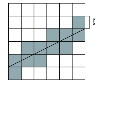
Figure 5. An example pixelation of a line with slope $\frac{1}{2}$

It is easy to see that the pixelation of an set can be fundamentally different from a set. For example, every pixelation of a line segment will have many corners (as long as the line is not parallel to the $x$ or $y$-axis.) This implies that as $\varepsilon$ becomes small, the total curvature of the boundaries of pixelations of a line segment will increase in an unbounded fashion. This contradicts the fact that the line itself has no curvature and shows that essential geometric features of the set are not preserved in the pixelation.

In fact, though it is more difficult to see, pixelations do not preserve the topological properties of the set. Consider the set $S$ consisting of a line of slope $\frac{1}{2}$ and a line of slope $1$ which both start at the origin. Then it can be shown that for every $\varepsilon$, $P_{\varepsilon}(S)$ contains a hole which prevents $P_{\varepsilon}(S)$ from being contractible (see Figure 6.) The position of the hole depends on $\varepsilon$, but it will always exist for any $\varepsilon$. This example is far from unique. In fact, by altering the slope of the two lines we can create a set whose pixelations contain any desired number of holes. This shows that pixelations do not preserve the topological properties of the underlying set.

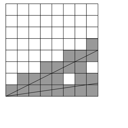
Figure 6. If $S$ consists of a line of slope $\frac{1}{2}$ and a line of slope $1$ starting at the origin, then $P_{\varepsilon}(S)$ is not contractible for any $\varepsilon$.

However, when $\varepsilon$ is very small, it is easy for the human eye to detect the kind of shape that probably generated a pixelation. Mathematically this corresponds to the fact that it is possible to create an approximation from the information in the pixelation which will respect topological and geometric features. The approximation can be algorithmically generated, but we delay defining it until much later in the paper (since the motivation for it rests on many properties of pixelations.)

The remainder of the paper will examine specifically what pixelations preserve and what they destroy. Furthermore it will explain how to recover the information “lost” in the process of creating a pixelation.

We end this section with a few basic properties of pixelations which will be useful.

Proposition 1.2.

For any two sets $U$ and $V$ we have

$$P_{\varepsilon}(U\cup V)=P_{\varepsilon}(U)\cup P_{\varepsilon}(V)$$

Proof.

This follows immediately from the definition of a pixelation as the union all pixels which intersect a set. $\hbox to0.0pt{$\sqcap$\hss}\sqcup$

Proposition 1.3.

For each $\varepsilon$ define $T_{\varepsilon}^{\infty}(S)$ to be

$$T_{\varepsilon}^{\infty}(S):=\{x\in\mathbb{R}^{2}:\exists p\in S\text{ such that }\|x-p\|_{\infty}\leq\varepsilon\}$$

i.e. the tube of radius $\varepsilon$ of $S$ in the $\|\bullet\|$ norm. Then

$$P_{\varepsilon}(S)\subset T_{\varepsilon}^{\infty}(S)$$

Proof.

Suppose $x\in P_{\varepsilon}(S)$. Then $\exists p\in S$ such that $x$ and $p$ lie within the same $\varepsilon$ pixel. But by the definition of pixels, this implies that $\|x-p\|_{\infty}\leq\varepsilon$. Therefore $x\in T_{\varepsilon}^{\infty}(S)$. $\hbox to0.0pt{$\sqcap$\hss}\sqcup$

2. Pixelations of Functions and First-Order Approximation

In order to reach our overall goal of recovering sufficiently nice sets from their pixelations, we must start by examining simple sets. The graphs of $C^{2}$ functions on compact domains provide a good starting point. We will find that in this case many analogues of basic theorems from calculus appear in a pixelated version, and these facts will allow us to approximate the graphs of these functions.

Before we proceed in our investigation we need to introduce a basic vocabulary that will be used throughout the paper.

Definition 2.1.

Fix $\varepsilon>0$ and a bounded set $S\subset\mathbb{R}^{2}$.

1. A point $a\in\mathbb{R}$ will be called $\varepsilon$-generic if $x\in\mathbb{R}\setminus\varepsilon\mathbb{Z}$. For such a point $a$ we denote by $I_{\varepsilon}(a)$ the interval of the form $[n\varepsilon,(n+1)\varepsilon]$, $n\in\mathbb{Z}$ that contains $a$.

2. For an interval $[a,b]\subset\mathbb{R}$ we define the vertical strip

   $$\mathcal{S}_{[a,b]}:=[a,b]\times\mathbb{R}$$

   For every $k\in\mathbb{Z}$ we denote by $\mathcal{S}_{\varepsilon,k}$ the vertical strip

   $$[k\varepsilon,(k+1)\varepsilon]\times\mathbb{R}=\mathcal{S}_{[k\varepsilon,(k+1)\varepsilon]}$$

   For any $\varepsilon$-generic point $a\in\mathbb{R}$ we denote by $\mathcal{S}_{\varepsilon}(a)$ the strip

   $$I_{\varepsilon}(a)\times\mathbb{R}=S_{\varepsilon,k},\;\;k:=\lfloor x/k\rfloor.$$

3. A column of $P_{\varepsilon}(S)$ is the intersection of $P_{\varepsilon}(S)$ with a vertical strip $\mathcal{S}_{\varepsilon,k}$, $k\in\mathbb{Z}$. The connected components of a column are called stacks.

4. For every $\varepsilon$-generic $a\in\mathbb{R}$, we define the column of a pixelation $P_{\varepsilon}(S)$ over $a$ to be the set

   $$C_{\varepsilon}(S,a):=\mathcal{S}_{\varepsilon}(a)\cap P_{\varepsilon}(S).$$

   In other words, $C_{\varepsilon}(S,a)$ is the union of the pixels in $P_{\varepsilon}(S)$ which intersect the vertical line $\{x=a\}$. When $S$ is the graph of a function $f$, we will use the notation $C_{\varepsilon}(f,a)$ to denote the column over $a$ of the pixelation $P_{\varepsilon}(f)$.

5. We define the top, bottom and respectively height of a column to be the quantities

   $$T_{\varepsilon}(S,a):=\sup\{y:(a,y)\in C_{\varepsilon}(S,a)\},$$

   $$B_{\varepsilon}(S,a):=\inf\{y:(a,y)\in C_{\varepsilon}(S,a)\},$$

   and respectively

   $$h_{\varepsilon}(S,a):=\frac{1}{\varepsilon}\bigl{(}\,T_{\varepsilon}(S,a)-B_{\varepsilon}(S,a)\,\bigr{)}.$$

$\hbox to0.0pt{$\sqcap$\hss}\sqcup$

Since stacks are constrained to be within the same column, a stack can usually be thought of as two pixels together with all the pixels that fall vertically in between them.

This language allows us to state an analogue of the Intermediate Value Theorem.

Theorem 2.2 (Pixelated Intermediate Value Theorem).

If $f:[a,b]\rightarrow\mathbb{R}$ is a continuous function, then for every $x\in[a,b]\setminus\varepsilon\mathbb{Z}$, the column $C_{\varepsilon}(f,x)$ consists of exactly one stack.

Proof.

We argue by contradiction. Suppose that the column $C_{\varepsilon}(f,x)$ has at least two stacks. This means that within the column over $x$ there are two stacks with a gap of empty pixels in between them. This implies that there exist an interval $[c\varepsilon,d\varepsilon]$, not contained in the range of $f$, and real numbers $x_{1},x_{2}\in I_{\varepsilon}(x)$ such that

$$f(x_{2})<c\varepsilon<d\varepsilon<f(x_{1}).$$

Since $f$ is continuous, this contradicts the Intermediate Value Theorem. Therefore the column over $x$ has only one stack. $\hbox to0.0pt{$\sqcap$\hss}\sqcup$

Note that the Pixelated Intermediate Value Theorem immediately implies that a cycle cannot appear in the pixelation of a continuous function. Therefore the pathological behavior witnessed in Appendix A will not occur in the pixelations of $C^{2}$ functions, which is our first hint that pixelations of $C^{2}$ functions are the nicest type of pixelation to work with.

This analogue of the Intermediate Value Theorem tells us that we can think of the pixelation of a function that assign a stack of pixels to each value in the domain of the function. The stacks themselves are worth investigating. To generate a stack in the pixelation, the function must attain values near the top and bottom of the stack within that column. This means that the average change of a function over a column must be related to the height of the column. This relation will be shown in the following two theorems. The first tells us that the height of a stack is bounded by the derivative of the function.

Proposition 2.3.

Let $f:[a,b]\rightarrow\mathbb{R}$ be a Lipschitz continuous function. We denote by $\|f^{\prime}\|_{\infty}$ the best Lipschitz constant, i.e.,

$$\|f^{\prime}\|_{\infty}:=\sup_{x\neq y}\frac{|f(x)-f(y)|}{|x-y|}.$$

Then for any $\varepsilon>0$ and any $x\in[a,b]\setminus\varepsilon\mathbb{Z}$ we have

$$h_{\varepsilon}(f,x)\leq||f^{\prime}||_{\infty}+2.$$

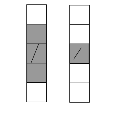
Figure 7. If the line on the left were any shorter it would generate the pixelation on the left. Thus, the minimum range of a function in a column is two less than the height of the column.

Proof.

We argue by contradiction. This means that there exist $\varepsilon>0$ and $x\in[a,b]\setminus\varepsilon\mathbb{Z}$ such that

$$h_{\varepsilon}(f,x)>||f^{\prime}||_{\infty}+1.$$ (2.1)

Set $n:=\lfloor x/\varepsilon\rfloor\in\mathbb{Z}$ so that $n\varepsilon<x<(n+1)\varepsilon$. The inequality (2.1) is equivalent to the condition

$$T_{\varepsilon}(f,x)-B_{\varepsilon}(f,x)>\varepsilon(||f^{\prime}||_{\infty}+2).$$

This implies that

$$\exists c,d\in\bigl{(}n\varepsilon,(n+1)\varepsilon\,\bigr{)}\;\;\mbox{such that}\;\;|f(c)-f(d)|>||f^{\prime}||_{\infty}\varepsilon,$$

because the pixelation can be one pixel higher or lower than the graph of $f$; see Figure 7. We have thus found $c$ and $d$ such that

$$\frac{|f(c)-f(d)|}{|c-d|}>\frac{||f^{\prime}||_{\infty}\varepsilon}{\varepsilon}=||f^{\prime}||_{\infty}$$

But this contradicts the definition of $\|f^{\prime}\|_{\infty}$. $\hbox to0.0pt{$\sqcap$\hss}\sqcup$

Remark 2.4.

(a) Observe that if $x\in[a,b]\cap\varepsilon\mathbb{Z}$ then

$$h_{\varepsilon}(f,x)\leq 2(\|f^{\prime}\|_{\infty}+1).$$

(b) The above theorem can be used to bound the height of a stack by the derivative of $f$ over that stack by considering the restriction of $f$ to that column. $\hbox to0.0pt{$\sqcap$\hss}\sqcup$

The next theorem suggests that the height of a stack is close, in a crude way, to the absolute value of the derivative in the column for sufficiently small $\varepsilon$. The intuition is that if $f$ is $C^{2}$, then any sufficiently small section of its graph will be very close to the graph of a line, and the height of a stack in the pixelation of the graph of a line must be very close to the slope of that line.

Proposition 2.5.

Let $f$ be a $C^{2}$ function on $[a,b]$. Then, for any $\varepsilon>0$ and any $x_{0}\in[a,b]\setminus\varepsilon\mathbb{Z}$ we have

$$|f^{\prime}(x_{0})|\leq h_{\varepsilon}(f,x_{0})|+\|f^{\prime\prime}\|_{\infty}\varepsilon+2.$$

Proof.

Recall that $I_{\varepsilon}(x_{0})$ indicates the interval of the form $[n\varepsilon,(n+1)\varepsilon]$, $n\in\mathbb{Z}$, that contains $x_{0}$. Let $L$ be the linearization of $f$ at $x_{0}$, i.e., the function

$$L:\mathbb{R}\rightarrow\mathbb{R},\;\;L(x):=(x-x_{0})f^{\prime}(x_{0})+f(x_{0}).$$

From Taylor’s Theorem we deduce that

$$|L(x)-f(x_{0})|\leq\frac{||f^{\prime\prime}||_{\infty}}{2}(x-x_{0})^{2}\leq\frac{1}{2}||f^{\prime\prime}||_{\infty}\varepsilon^{2}\leq\varepsilon,\;\;\forall x\in I_{\varepsilon}(x_{0})\cap[a,b].$$

This implies that

$$T(L,x_{0})\leq T(f,x_{0})+\frac{1}{2}\|f^{\prime\prime}\|_{\infty}\varepsilon^{2}+\varepsilon,\;\;B(L,x_{0})\geq B(f,x_{0})-\frac{1}{2}\|f^{\prime\prime}\|_{\infty}\varepsilon^{2}-\varepsilon.$$

Hence,

$$h_{\varepsilon}(L,x_{0})\leq h(f,x_{0})+\|f^{\prime\prime}\|_{\infty}\varepsilon+2.$$

On the other hand, $L$ changes by $f^{\prime}(x_{0})\varepsilon$ over the width of a pixel, which implies

$$|f^{\prime}(x_{0})|\leq h_{\varepsilon}(L,x_{0})$$

$\hbox to0.0pt{$\sqcap$\hss}\sqcup$

We would now like to approximate $f$ through its pixelations. An intuitive way to do this is by creating a $PL$ function whose graph lies within $P_{\varepsilon}(f)$, since this approximation would generate a similar pixelation. However, in practice this method requires making many choices, and it can be cumbersome to check that the graph of the function lies within the pixelation of $f$. A better approach is to form a $PL$ function by connecting points within $P_{\varepsilon}(f)$ by straight line segments. In order to preserve higher order properties of the function, we must be careful when choosing these points.

For example, suppose that the vertices of the $PL$ approximation are centers of the top pixels in each column. Then the slopes of each line making up the $PL$ function would have integer slopes, and could never approximate the derivative of $f$ arbitrarily well. We could increase the accuracy of the approximation by connecting the maxima of every other column, or every third column. However, doing this decreases the speed in which the approximation converges pointwise to $f$. This is the central tension involved in approximating a function from its pixelation.

Before we further describe how to approximate a function from its pixelation, we show how to at least find the average change of the function, i.e., the slope of the secant line connecting the first and last points of $f$.

Theorem 2.6.

Let $f$ be a $C^{2}$ function on the interval $[a,b]$. Fix $\varepsilon>0$. Let $c,d\in\mathbb{R}$ such that $(a,c)\in P_{\varepsilon}(f)$ and $(b,d)\in P_{\varepsilon}(f)$.

$$g_{\varepsilon}(x):=(x-a)\frac{d-c}{b-a}+c.$$

Then

$$|f(x)-g_{\varepsilon}(x)|\leq 7(||f^{\prime}||_{\infty}+2)\varepsilon+3||f^{\prime}||_{\infty}(b-a)+||f^{\prime\prime}||_{\infty}(b-a)^{2}$$ (2.2)

and

$$|f^{\prime}(x)-g_{\varepsilon}^{\prime}(x)|=|f^{\prime}(x)-\frac{d-c}{b-a}|\leq(b-a)||f^{\prime\prime}||_{\infty}+\frac{2(||f^{\prime}||_{\infty}+2)\varepsilon}{(b-a)},$$ (2.3)

for all $x\in[a,b]$.

Proof.

Note that it suffices to prove the above inequalities in the special case when $x\in[a,b]\setminus\varepsilon\mathbb{Z}$. For ease of notation let

$$M:=||f^{\prime}||_{\infty},\;\;N:=||f^{\prime\prime}||_{\infty},\;\;m_{f}:=\frac{f(b)-f(a)}{b-a}$$

and note that $m_{f}$ is the slope of the secant line to $f$ over the interval $[a,b]$. Define

$$m_{g}:=\frac{d-c}{b-a},$$

and note that this is the slope of $g_{\varepsilon}$. Note that $c$ and $d$ differ from $f(a)$ and $f(b)$ by at most the height of a stack.

Lemma 2.7.

With $m_{f}$ and $m_{g}$ defined as above,

$$|m_{f}-m_{g}|\leq\frac{2(||f^{\prime}||_{\infty}+2)\varepsilon}{b-a}.$$ (2.4)

Proof of Lemma 2.4. Theorem 2.3 implies that a height of a stack in $P_{\varepsilon}(f)$ is at most $M+2$ so

$$|f(a)-c|,|f(b)-d|\leq(M+2)\varepsilon.$$

This immediately implies

$$|m_{f}-m_{g}|=|\frac{f(b)-f(a)}{b-a}-\frac{d-c}{b-a}|\leq\frac{1}{b-a}(|f(b)-d|+|f(a)-a|)\leq\frac{2(M+2)\varepsilon}{b-a}. \hbox to0.0pt{$\sqcap$\hss}\sqcup$$

The Mean Value Theorem implies that $\exists\xi\in[a,b]$ such that $f^{\prime}(\xi)=m_{f}$. Let $h(x)$ be the linearization of $f$ at $\xi$,i.e.,

$$h(x):=(x-\xi)m+f(\xi).$$

Thus we have

$$|g_{\varepsilon}(x)-h(x)|=|(x-a)m_{g}+c-(x-\xi)m_{f}-f(\xi)|\\ \leq|(x-a)m_{g}-(x-\xi)m_{f}|+|d-f(\xi)|$$ (2.5)

First we will bound the first term on the right hand side of (2.5).

$$|(x-a)m_{g}-(x-\xi)m_{f}|=|(x-a)m_{g}-(x-\xi)m_{g}+(x-\xi)m_{g}-(x-\xi)m_{f}|$$

$$\leq|m_{g}|(|x-a|+|x-\xi|)+|m_{g}-m_{f}|(|x-\xi|)$$

To proceed further we need to use the following facts.

• $|x-a|,|x-\xi|\leq|b-a|$.

• $|m_{g}-m_{f}|\leq\frac{2(M+2)\varepsilon}{b-a}$.

• Since $|m_{f}|\leq M$, we have

  $$|m_{g}|\leq M+\frac{2(M+2)\varepsilon}{b-a}.$$

Therefore

$$|(x-a)m_{g}-(x-\xi)m_{f}|\leq 2(b-a)(M+\frac{2(M+2)\varepsilon}{b-a})+(b-a)\frac{2(M+2)\varepsilon}{b-a}$$

$$=2M(b-a)+6(M+2)\varepsilon.$$

Now we bound the other term from (2.5), $|c-f(\xi)|=|c-h(\xi)|$. We have

$$|c-f(\xi)|\leq|c-f(a)|+|f(a)-h(a)|+|h(a)-h(\xi)|.$$

Note that $|f(a)-c|\leq(M+2)\varepsilon$, since stacks are at most $M+2$ pixels tall. Taylor’s Theorem implies that

$$|f(a)-h(a)|\leq\frac{N(b-a)^{2}}{2}.$$

Finally $|h(\xi)-h(a)|\leq M(b-a)$, since $h$ has slope at most $M$, and $|\xi-a|\leq(b-a)$. We conclude that

$$|f(\xi)-c|\leq(M+2)\varepsilon+\frac{N(b-a)^{2}}{2}+M(b-a).$$

Combining all of these bounds in (2.5) we deduce

$$|g_{\varepsilon}(x)-h(x)|\leq 3M(b-a)+7(M+2)\varepsilon+\frac{N(b-a)^{2}}{2}.$$

Finally,

$$|f(x)-h(x)|\leq\frac{N(b-a)^{2}}{2},$$

so that

$$|f(x)-g(x)|\leq 7(M+2)\varepsilon+3M(b-a)+N(b-a)^{2}.$$

which is the bound (2.2).

The bound (2.3) is obtained as follows.

$$|f^{\prime}(x)-g_{\varepsilon}^{\prime}(x)|=|f^{\prime}(x)-m_{g}|\leq|m_{g}-m_{f}|+|m_{f}-f^{\prime}(x)|$$

$$\stackrel{{\scriptstyle(\ref{eq: 281})}}{{\leq}}\frac{2(M+2)\varepsilon}{b-a}+|f^{\prime}(\xi)-f^{\prime}(x)|\leq\frac{2(M+2)\varepsilon}{b-a}+N\varepsilon.$$

$\hbox to0.0pt{$\sqcap$\hss}\sqcup$

This Theorem tells us that the slope of a secant line to $f$ can be accurately approximated up to its derivative (by restricting $f$ to various intervals we can approximate any secant line.) We would like approximate $f$ through the use of multiple secant lines. However to accurately approximate a small secant line, we will need $\varepsilon$ to be very small. On the other hand, to accurately approximate $f$ we will need to use many (and therefore small) secant lines. Thus we will need to know the size of a secant line that can be accurately approximated for a given $\varepsilon$. Before we can describe how to go about this process, however, we will need additional terms.

Definition 2.8.

Fix $\varepsilon>0$ and a bounded set $S$.

1. An $\varepsilon$-profile of $S$ is a set $\Pi_{\varepsilon}$ of points in the plane with the following properties.

   1. Each point in $\Pi_{\varepsilon}$ is the center of an $\varepsilon$-pixel that intersects $S$.

   2. Every column of $P_{\varepsilon}(S)$ contains precisely one point of $\Pi_{\varepsilon}$.

2. A top/bottom $\varepsilon$-profile is a profile consisting of the centers of the highest/lowest pixels in each column of $P_{\varepsilon}(S)$.

3. An $\varepsilon$-sample of $S$ is a subset of an $\varepsilon$-profile.

$\hbox to0.0pt{$\sqcap$\hss}\sqcup$

Definition 2.9.

Suppose $p_{1},\dotsc,p_{N}$ is a finite sequence of points in $\mathbb{R}^{2}$. (The points need not be distinct). We denote by

$$\langle p_{1},p_{2},\dotsc,p_{n}\rangle$$

the $PL$ curve defined as the union of the straight line segments $[p_{1},p_{2}],\dotsc,[p_{n-1},p_{n}]$. $\hbox to0.0pt{$\sqcap$\hss}\sqcup$

Observe that each $\varepsilon$-profile $\Pi_{\varepsilon}$ of a set is equipped with a linear order $\preceq$. More precisely if $p_{1},p_{2}=(x_{2},y_{2})$ are points in $\Pi_{\varepsilon}$, then

$$p_{1}\preceq p_{2}\Longleftrightarrow x(p_{1})\leq x(p_{2}),$$

where $x:\mathbb{R}^{2}\rightarrow\mathbb{R}$ denotes the projection $(x,y)\mapsto x$. In particular, this shows that any $\varepsilon$-sample of $S$ carries a natural total order.

If $\Xi$ is an $\varepsilon$-sample of $S$, then the $PL$-interpolation determined by sample $\Xi$ is the continuous, piecewise linear function $L=L_{\Xi}$ obtained as follows.

• Arrange the points in $\Xi$ in increasing order, with respect to the above total order,

  $$V=\{\xi_{0}\prec\xi_{1}\prec\xi_{2}\prec\cdots\prec\xi_{n}\},\;\;n+1=|\Xi|.$$

• The graph of $L_{\Xi}$ is the $PL$-curve $\langle\xi_{0},\xi_{1},\dotsc,\xi_{n}\rangle$.

In applications, the sample sets $\Xi$ will be chosen to satisfy certain regularity.

Definition 2.10.

1. If $\sigma$ is a positive integer and $\Pi_{\varepsilon}$ is an $\varepsilon$-profile, then an $\varepsilon$-sample with spread $\sigma$ is a subset

   $$\Xi=\{\xi_{0}\prec\cdots\prec\xi_{n}\}\subset\Pi_{\varepsilon}(S)$$

   such that the following hold.

   • The points $\xi_{0}$ and $\xi_{n}$ are the left and rightmost points in the profile. (That is for each $p\in\Pi_{\varepsilon}$, $x(\xi_{0})\leq x(p)\leq x(\xi_{n})$.)

   • For any $p\in\Pi_{\varepsilon}$, there exists $\xi\in\Xi$ such that $|x(p)-x(\xi)|<\varepsilon\sigma$.

   • $$\frac{1}{2}\sigma\leq\frac{1}{\varepsilon}|x(\xi_{k})-x(\xi_{k-1})|\leq\sigma,\;\;\forall k=1,\dotsc,n.$$

2. A spread is an increasing function $\varepsilon\mapsto\sigma(\varepsilon)$ from the positive real numbers to the positive integers with the following properties:

   1. $\lim_{\varepsilon\searrow 0}\sigma(\varepsilon)=\infty$

   2. $\lim_{\varepsilon\searrow 0}\varepsilon\sigma(\varepsilon)=0$

$\hbox to0.0pt{$\sqcap$\hss}\sqcup$

The next theorem tells how to approximate $f$ using profiles and spreads while maintaining first order properties.

Theorem 2.11.

Let $f:[a,b]\rightarrow\mathbb{R}$ be a $C^{2}$-function and $\sigma(\varepsilon)$ be a spread function. Fix $\varepsilon>0$ and let $\Xi$ be an $\varepsilon$-sample of the graph of $f$ with spread $\sigma(\varepsilon)$,

$$\Xi=\{\xi_{0}\prec\xi_{1}\prec\cdots\prec\xi_{n}\},\;\;\xi_{k}=(x_{k},y_{k}),\;\;k=0,1,\dotsc,n.$$

Denote by $f_{\Xi}:[x_{0},x_{n}]\rightarrow\mathbb{R}$ the $PL$-interpolation determined by $\Xi$. Then

$$\bigl{|}\,f(x)-f_{\Xi}(x)\,\bigr{|}\leq 7\bigl{(}\,\|f^{\prime}\|_{\infty}+2\,\bigr{)}\varepsilon+3\|f^{\prime}\|_{\infty}\varepsilon\sigma(\varepsilon)+\|f^{\prime\prime}\|_{\infty}(\varepsilon\sigma(\varepsilon))^{2},\;\;\forall x\in[a,b]\cap[x_{0},x_{n}],$$

and

$$|f^{\prime}(x)-f_{\Xi}^{\prime}(x)|\leq\frac{4(\|f^{\prime}\|_{\infty}+2)}{\sigma(\varepsilon)}+\|f^{\prime\prime}\|_{\infty}\varepsilon\sigma(\varepsilon),$$

for all $x\in[a,b]\cap[x_{0},x_{n}]\setminus\{x_{0},\dotsc,x_{n}\}$. In particular, if

$$\lim_{\varepsilon\searrow 0}\varepsilon\sigma(\varepsilon)=0\;\;\mbox{and}\;\;\lim_{\varepsilon\searrow 0}\sigma(\varepsilon)=\infty,$$

then as $\varepsilon\searrow 0$, $f_{\Xi}$ converges to $f$ in the Sobolev norm $W^{1,p}$ for all $p\in[1,\infty)$.

Proof.

Let $x\in[x_{0},x_{n}]$ and $k\in\{0,1,\dotsc,(n-1)\}$ such that $x\in[x_{k},x_{k+1}]$. On this subinterval, the function $f_{\Xi}$ is defined by

$$f_{\Xi}(x):=(x-x_{k})\frac{y_{k+1}-y_{k}}{x_{k+1}-x_{k}}+y_{k}.$$

Thus $f_{\Xi}$ is a function of the type described in Theorem 2.6, where

$$a=x_{k},\;\;b=x_{k+1},\;\;c=y_{k},\;\;d=y_{k+1}.$$

Noting that

$$\frac{1}{2}\varepsilon\sigma(\varepsilon)\leq b-a\leq\varepsilon\sigma(\varepsilon),$$

we obtain the desired error bounds.

Now suppose that $\lim_{\varepsilon\searrow 0}\sigma(\varepsilon)\varepsilon=0$ and $\lim_{\varepsilon\searrow 0}\sigma(\varepsilon)=\infty$. Then note that every term in both the error bounds of $\bigl{|}f-f_{\Xi}\bigr{|}$ and $\bigl{|}f-f_{\Xi}^{\prime}\bigr{|}$ is a constant multiplied by $\varepsilon$, $\frac{1}{\sigma(\varepsilon)}$, or $\varepsilon\sigma(\varepsilon)$ all of which converge to $0$ as $\varepsilon\searrow 0$. This implies that

$$\lim_{\varepsilon\rightarrow 0}\int_{a}^{b}\left(|f(x)-f_{\Xi}(x)|^{p}+|f^{\prime}(x)-f_{\Xi}^{\prime}(x)|^{p}\right)dx=0,\;\;\forall 1\leq p<\infty.$$

Therefore $f_{\Xi}$ converges to $f$ in the Sobolev $W^{1,p}$ norm.

$\hbox to0.0pt{$\sqcap$\hss}\sqcup$

This theorem allows us to approximate $C^{2}$ functions using only their pixelations. Note that any profile can be chosen for the approximation. We can see this in the pixelation by noting that the top profile and bottom profile both converge to the graph of the function, so any profile chosen in between will be squeezed onto the graph.

To ensure the correct convergence on the derivative, we only need the two basic features of a spread: that as $\varepsilon\searrow 0$, $\sigma(\varepsilon)\to\infty$ and $\varepsilon\sigma(\varepsilon)\searrow 0$. In general we would like the spread to increase quickly, so as to get an accurate approximation on the derivative. The two conditions on the spread mean that the quickest increasing spread will look like $\lceil\varepsilon^{\frac{-1}{1+r}}\rceil$ where $r>0$.

3. Approximations of Elementary Regions and Curvature Approximation

In this section we use the properties of pixelations of functions to study the pixelations of simple two dimensional sets. We deal with the simplest case: that of a region between the graphs of two $C^{2}$ functions.

Definition 3.1.

A subset $S\subset\mathbb{R}^{2}$ is said to be elementary (with respect to the $x$-axis) if its can be defined as

$$S=S(\beta,\tau):=\bigl{\{}\,(x,y):x\in[a,b],\beta(x)\leq x\leq\tau(x)\,\bigr{\}},$$

where $\beta,\tau:[a,b]\rightarrow\mathbb{R}$ are $C^{2}$ functions such that $\beta(x)\leq\tau(x)$, $\forall x\in[a,b]$. The function $\beta$ is called the bottom of $S$ while $\tau$ is called the top of $S$. Note that this includes the situation where $\beta\equiv\tau$, in which case $P_{\varepsilon}(S)=P_{\varepsilon}(\beta)=P_{\varepsilon}(\tau)$. $\hbox to0.0pt{$\sqcap$\hss}\sqcup$

In the remainder of this section $S$ will indicate an elementary set. We first note that like the pixelation of a function, each column of $P_{\varepsilon}(S)$ contains only one stack:

Proposition 3.2.

If $S=S(\beta,\tau)$ is an elementary set, then for every $x\in[a,b]\setminus\varepsilon\mathbb{Z}$, the column $C_{\varepsilon}(S,x)$ consists of exactly one stack.

Proof.

Fix an $\varepsilon$-generic $x\in[a,b]$. By Theorem 2.2 the columns $C_{\varepsilon}(\beta,x)$ and $C_{\varepsilon}(\tau,x)$ consist of single stacks. If these two columns intersect, then the conclusion is obvious. If they do not intersect, then any pixel in the strip $S_{\varepsilon}(x)$ situated below the stack $C_{\varepsilon}(\tau,x)$ and above the stack $C_{\varepsilon}(\beta,x)$ is a pixel of $P_{\varepsilon}(S)$. This again proves that the column $C_{\varepsilon}(S,x)$ consists of a single stack. $\hbox to0.0pt{$\sqcap$\hss}\sqcup$

Definition 3.3.

Fix $\varepsilon>0$ and an elementary set $S=S(\beta,\tau)$.

1. An $\varepsilon$-upper/lower profile of $S$ is a profile of the $\varepsilon$-pixelation of the top/bottom function. An $\varepsilon$-upper/lower sample is a sample of an upper/lower profile.

2. An $\varepsilon$-upper profile $\Pi^{+}_{\varepsilon}$ is said to be compatible with an $\varepsilon$-lower profile $\Pi^{-}_{\varepsilon}$ if $p^{+}\in\Pi^{+}_{\varepsilon}$ and $p^{-}\in\Pi_{\varepsilon}^{-}$ lie in the same column of $P_{\varepsilon}(S)$ we have $p^{+}\in\Pi^{+}_{\varepsilon}$ and $p^{-}\in\Pi_{\varepsilon}^{-}$ lie in the same column of $P_{\varepsilon}(S)$ we have

   $$y(p^{-})\leq y(p^{+}).$$

3. An $\varepsilon$-upper sample $\Xi^{+}$ is said to be compatible with an $\varepsilon$-lower sample $\Xi^{-}$, if the following hold.

   • There exist compatible $\varepsilon$-upper/lower profiles $\Pi^{\pm}$ such that $\Xi^{\pm}\subset\Pi^{\pm}$.

   • A strip $\mathcal{S}_{\varepsilon,k}$ contains a point in $\Xi^{+}$ if and only if it also contains a point in $\Xi^{-}$.

4. Suppose that $\Xi^{\pm}_{\varepsilon}$ are compatible upper/lower samples of $S$

   $$\Xi^{\pm}_{\varepsilon}=\{\xi_{0}^{\pm}\prec\xi_{1}^{\pm}\prec\cdots\prec\xi_{n}^{\pm}\}.$$

   The $PL$-approximation of $S$ determined by these two samples is the $PL$-set bounded by the simple closed $PL$-curve

   $$\langle\xi_{0}^{-},\xi_{1}^{-},\dotsc,\xi_{n}^{-},\xi_{n}^{+},\xi_{n-1}^{+},\dotsc,\xi_{0}^{+},\xi_{0}^{-}\rangle.$$

   We denote this approximation by $|S(\Xi_{\varepsilon}^{-},\Xi_{\varepsilon}^{+})|$. $\hbox to0.0pt{$\sqcap$\hss}\sqcup$

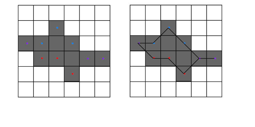
Figure 8. An example of PL approximation. The left figure shows a pixelation of an elementary subset, together with a compatible upper and lower profile. The upper profile is indicated in blue while the lower profile is in red. The right figure shows the PL approximation of compatible samples of these approximations with spread 2. The PL approximation for the combined upper and lower samples would be the region in between the upper and lower approximations.

These definitions are extensions of the ideas of profiles, samples and PL approximations found in section 2. Note that the upper and lower profiles are defined from the pixelations of the top and bottom function, which might not be known. However, from the definition of an elementary set, every pixel on the top of a column must intersect the pixelation of the upper function and similarly every pixel at the bottom of a column must intersect the lower function. Therefore, an upper profile can be thought of as a profile chosen from the top pixels of $P_{\varepsilon}(S)$ and a lower profile can be thought of as a profile chosen from the lower pixels of $P_{\varepsilon}(S)$.

In section 2 we noted that the PL approximation preserves first order properties for a good choice of spread. For elementary sets, we would like to prove something stronger. Namely, we would like to show that the total curvature of the set is preserved for good choice of spread.

The total curvature of a $C^{2}$ immersion $\gamma:[a,b]\rightarrow\mathbb{R}^{2}$ is defined as follows. Define a $C^{1}$-function $\theta:[a,b]\rightarrow\mathbb{R}$ such that

$$\frac{1}{|\dot{\gamma}(t)|}\dot{\gamma}(t)=(\cos(\theta(t),\sin(\theta(t))),$$

where a dot $\dot{}$ denotes the $t$-derivative. We set

$$\kappa(t):=|\dot{\theta}(t)|.$$

The scalar $\kappa(t)$ is called the curvature of $\gamma$ at the point $\gamma(t)$. We define the total curvature of $\gamma$ to be

$$K(\gamma):=\int_{a}^{b}\kappa(t)\,dt.$$

Suppose now that $\gamma:[a,b]\rightarrow\mathbb{R}^{2}$ continuous and piecewise $C^{2}$-immersion, i.e., there exist a finite subset $\{t_{0},\dotsc,t_{\nu}\}\subset[a,b]$, $t_{i-1}<t_{i}$, for

$$a=t_{0}<t_{1}<\cdots<t_{\nu-1}<t_{\nu}=b$$

such that the restriction $\gamma_{i}:=\gamma|_{[[t_{i-1},t_{i}]}$ is a $C^{2}$-immersion for any $i=1,\dotsc,\nu$. The curvature of $\gamma$ at a jump point $\gamma(t_{i})$ is the quantity

$$\kappa(t_{i})=|\theta(t_{i}^{+})-\theta(t_{i}^{-})|:=|\lim_{t\searrow t_{i}}\theta(t)-\lim_{t\nearrow t_{i}}\theta(t)|.$$

We define the total curvature of $\gamma$ to be

$$\begin{split}K(\gamma)&:=\sum_{i=1}^{\nu}K(\gamma_{i})+\sum_{i=1}^{\nu-1}\kappa(t_{i})\\ &+\begin{cases}0,&\gamma(b)\neq\gamma(a)\\ |\theta(t_{0}^{+})-\theta(t_{\nu}^{-})|,&\gamma(b)=\gamma(a).\end{cases}\end{split}$$

For more details we refer to [18] and [20, §2.2].

Proposition 3.4.

Let $h:[a,b]\rightarrow\mathbb{R}$ be a $C^{2}$ function. Fix a spread $\sigma$ satisfying the properties

$$\lim_{\varepsilon\searrow 0}\varepsilon\sigma(\varepsilon)^{2}=\infty,$$ (3.1a)

$$\lim_{\varepsilon\searrow 0}\varepsilon\sigma(\varepsilon)=0.$$ (3.1b)

For every $\varepsilon>0$ let $\Xi_{\varepsilon}$ be a $\varepsilon$-sample spread $\sigma$. We denote by $h_{\varepsilon}$ be the PL interpolation of $\Xi_{\varepsilon}$. Then

$$\lim_{\varepsilon\searrow 0}K(\Gamma_{h_{\varepsilon}})=K(\Gamma_{h}),$$

where for any function $f$ we denote by $\Gamma_{f}$ its graph.

Proof.

Let $X_{\varepsilon}$ be the ordered set of $x$-values of the sample $\Xi_{\varepsilon}$,

$$X_{\varepsilon}=\{x_{0}<x_{1}<\dots<x_{n}\}\subset[a,b],$$

and set

$$p_{i}:=(x_{i},h(x_{i}))\in\Gamma_{h}.$$

Define $s_{\varepsilon}$ to be the PL function with graph $\langle p_{0},p_{1},\dotsc,p_{n}\rangle$. We will prove two things.

$$\lim_{\varepsilon\rightarrow 0}\left(\,K(h_{\varepsilon})-K(s_{\varepsilon})\,\right)=0,$$ (3.2a)

$$\lim_{\varepsilon\rightarrow 0}K(s_{\varepsilon})=K(h).$$ (3.2b)

Proof of (3.2a). For $1\leq i\leq n$ let $m_{i}^{h}$ indicate the slope of the $i$-th line segment of $h_{\varepsilon}$ and $m_{i}^{s}$ indicate the slope of the $i$-th line segment of $s_{\varepsilon}$, i.e., the slope over the interval $[x_{i-1},x_{i}]$.

Since $h_{\varepsilon}$ has spread $\sigma$, the width of the interval $[x_{i-1},x_{i}]$ is at most $\varepsilon\sigma$. Then since $m_{i}^{h}$ is the slope of a line connecting two points in the sample $H_{\varepsilon}$, and $m_{i}^{s}$ is the slope of the secant line over the same interval, Lemma 2.4 implies that

$$|m_{i}^{h}-m_{i}^{s}|\leq 2\frac{||h^{\prime}||_{\infty}+2}{\sigma(\varepsilon)}$$ (3.3)

In particular, $|m_{i}^{h}-m_{i}^{s}|\to 0$ as $\varepsilon\to 0$ since $\sigma\to\infty$.

Define $\theta_{i}^{h}\in(-\frac{\pi}{2},\frac{\pi}{2})$ as the angle that the $(i+1)$-st line component of $s_{\varepsilon}$ makes with the $x$-axis and likewise $\theta_{i}^{s}\in(-\frac{\pi}{2},\frac{\pi}{2})$ as the angle that the $(i+1)$-st line component of $s$ makes with the $x$-axis. More precisely,

$$\tan(\theta_{i}^{h})=m_{i}^{h},\;\;\tan(\theta_{i}^{s})=m_{i}^{s}.$$

Therefore, the difference formula for tangent implies:

$$\frac{m_{i}^{h}-m_{i}^{s}}{1+m_{i}^{h}m_{i}^{s}}=\tan(\theta_{i}^{h}-\theta_{i}^{s})$$

so that

$$\theta_{i}^{h}-\theta_{i}^{s}=\arctan\left(\frac{m_{i}^{h}-m_{i}^{s}}{1+m_{i}^{h}m_{i}^{s}}\right).$$ (3.4)

Now, the estimate (3.3) implies that for small $\varepsilon$, we have

$$\left|\frac{m_{i}^{h}-m_{i}^{s}}{1+m_{i}^{h}m_{i}^{s}}\right|\leq 4\frac{\left(\|h^{\prime}\|_{\infty}+2\right)}{\sigma(\varepsilon)}.$$

Indeed, the denominator is at least $\frac{1}{2}$ because, for $\varepsilon$ sufficiently small, we have

$$1+m_{i}^{h}m_{i}^{s}=1+m_{i}^{h}\left(\,m_{i}^{h}+O\left(\sigma(\varepsilon)^{-1}\right)\,\right)$$

$$=1+(m_{i}^{h})^{2}+m_{i}^{h}O\left(\sigma(\varepsilon)^{-1}\right)=1+(m_{i}^{h})^{2}+O\left(\|h^{\prime}\|_{\infty}\sigma(\varepsilon)^{-1}\right).$$

Then, using the Taylor expansion of $\arctan$ around $0$, we have

$$\delta_{i}:=\theta_{i}^{h}-\theta_{i}^{s}=O\left(\frac{1}{\sigma(\varepsilon)}\right).$$ (3.5)

Recall that

$$K(s_{\varepsilon})=\sum_{i=1}^{n}\left|\,\theta_{i}^{s}-\theta_{i-1}^{s}\,\right|,\;\;K(h_{\varepsilon})=\sum_{i=1}^{n}\left|\,\theta_{i}^{h}-\theta_{i-1}^{h}\,\right|.$$

and we deduce that

$$\left|K(s_{\varepsilon})-K(h_{\varepsilon})\right|\leq\sum_{i=1}^{n}(|\delta_{i}|+|\delta_{i-1}|).$$

Note that since $\Xi_{\varepsilon}$ has spread $\sigma$,

$$n=O\left(\frac{1}{\varepsilon\sigma}\right)$$

and (3.5) implies

$$\sum_{i=1}^{n}(|\delta_{i}|+|\delta_{i-1}|)=O\left(\frac{1}{\varepsilon\sigma(\varepsilon)^{2}}\right).$$

Since we have assumed that $\lim_{\varepsilon\searrow}\varepsilon\sigma(\varepsilon)^{2}=\infty$, the last estimate implies (3.2a).

Proof of (3.2b). Define the function $\theta$ by the equation:

$$\frac{1}{|1+(h^{\prime}(x))^{2}|}\left(1,h^{\prime}(x)\right)=(\cos(\theta(x)),\sin(\theta(x)))$$

The function $\theta(x)$ gives the angle between the $x$-axis and the tangent line of $h$ at the point $x$. As before let $m_{i}^{s}$ indicate the slope of the $i$-th line segment of $s_{\varepsilon}$ and $\theta_{i}^{s}$ be the angle that the $i$-th line segment of $s_{\varepsilon}$ makes with the $x$-axis. The Mean Value Theorem implies that for each $i$ there exists a $\xi_{i}$ on $[x_{i-1},x_{i}]$ such that

$$m_{i}^{s}=h^{\prime}(\xi_{i})$$

It then follows that

$$\theta_{i}^{s}=\theta(\xi_{i})$$

since $\tan(m_{i}^{s})=\theta_{i}^{s}$ and $\tan(h^{\prime}(\xi_{i}))=\theta(\xi_{i})$. Furthermore, for each $i>1$, the Mean Value Theorem guarantees the existence of a $\zeta_{i}$ on $[\xi_{i-1},\xi_{i}]$ such that

$$\theta^{\prime}(\zeta_{i})=\frac{\theta(\xi_{i})-\theta(\xi_{i-1})}{\xi_{i}-\xi_{i-1}}$$

Recall that the total curvature of $s_{\varepsilon}$ is calculated by the summation:

$$K(s_{\varepsilon})=\sum_{i=2}^{n}|\theta_{i}^{s}-\theta_{i-1}^{s}|$$

Using the definitions of $\xi_{i}$ and $\zeta_{i}$ we find that

$$K(s_{\varepsilon})=\sum_{i=2}^{n}|\theta(\xi_{i})-\theta(\xi_{i-1})|=\sum_{i=2}^{n}\left|\frac{\theta(\xi_{i})-\theta(\xi_{i-1})}{\xi_{i}-\xi_{i-1}}\right|(\xi_{i}-\xi_{i-1})=\sum_{i=2}^{n}|\theta^{\prime}(\zeta_{i})|(\xi_{i}-\xi_{i-1})$$ (3.6)

Note that last sum in (3.6) is almost a Riemann sum for $|\theta^{\prime}|$. It is not a Riemann sum because the values $\{\xi_{1},\xi_{2},\dots,\xi_{n}\}$ do not form a partition of $[a,b]$ (since $\xi_{1}\geq a$ and $\xi_{n}\leq b$.) However, it is true that:

$$\lim_{\varepsilon\searrow 0}\left(|\theta^{\prime}(a)|(\xi_{1}-a)+\sum_{i=2}^{n}|\theta^{\prime}(\zeta_{i})|(\xi_{i}-\xi_{i-1})+|\theta^{\prime}(b)|(b-\xi_{n})\right)=\int_{a}^{b}|\theta^{\prime}(x)|dx$$ (3.7)

Both $(b-\xi_{n})$ and $(\xi_{1}-a)$ are intervals of size at most $\varepsilon\sigma(\varepsilon)$ (since our sample was chosen with spread $\sigma$.) Therefore both of these terms vanish as $\varepsilon\to 0$ (by our constraint on $\sigma$.) Therefore equation (3.7) simplifies to

$$\lim_{\varepsilon\searrow 0}\left(\sum_{i=2}^{n}|\theta^{\prime}(\zeta_{i})|(\xi_{i}-\xi_{i-1})\right)=\int_{a}^{b}|\theta^{\prime}(x)|dx$$ (3.8)

Combining (3.8) with (3.6) shows that

$$\lim_{\varepsilon\searrow 0}K(s_{\varepsilon})=\int_{a}^{b}|\theta^{\prime}(x)|dx=K(h)$$

which proves (3.2b).

Given both (3.2a) and (3.2b) we simply note that as $\varepsilon\to 0$ $K(h_{\varepsilon})$ approaches $K(s_{\varepsilon})$ which in turn approaches $K(h)$. $\hbox to0.0pt{$\sqcap$\hss}\sqcup$

In applications, it will be necessary to deal with sets which resemble elementary sets, but whose boundaries are possibly only piecewise $C^{2}$. Let us define precisely the notion of piecewise $C^{2}$ function.

Definition 3.5.

A function $f:[a,b]\rightarrow\mathbb{R}$ is said to be piecewise $C^{2}$ if there exists a finite set

$$S=\bigl{\{}a=s_{0}<s_{1}<\cdots<s_{\ell}=b\,\bigr{\}},$$

such that the following hold.

1. The function $f$ is continuous.

2. For any $j=1,\dotsc,\ell$, and any $k=1,2$ the restriction of $f$ to the open interval $(s_{j-1},s_{j})$ is a $C^{2}$ function and the limits

   $$\lim_{x\searrow s_{j-1}}f^{(k)}(x),\;\;\lim_{x\nearrow s_{j}}f^{(k)}(x)$$

   exist and are finite.

We say that $S$ is the singular set of $f$ and that the points $C_{j}=(s_{j},f(s_{j}))$, $j=0,\dotsc,\ell$ are the corners of the graph of $f$. The integer $\ell$ is called the length of the singularity set. $\hbox to0.0pt{$\sqcap$\hss}\sqcup$

Proposition 3.6.

Suppose that $f:[a,b]\rightarrow\mathbb{R}$ is a piecewise $C^{2}$ function with singular set

$$S:=\bigl{\{}a=s_{0}<s_{1}<\cdots<s_{\ell}=b\,\bigr{\}}.$$

Fix a spread satisfying the properties (3.1a) and (3.1b). For every $\varepsilon>0$ let $\Xi_{\varepsilon}$ be an $\varepsilon$-sample with spread $\sigma$ satisfying (3.1a) and (3.1b). For any $\varepsilon>0$ we denote by $f_{\varepsilon}$ be the PL interpolation of $\Xi_{\varepsilon}$. Then

$$\lim_{\varepsilon\searrow 0}K(\Gamma_{f_{\varepsilon}})=K(\Gamma_{f}).$$

Proof.

We will follow the same strategy as in the proof of Proposition 3.4, with some expected modifications due to the presence of singularities. For the clarity of exposition we will assume that the length $\ell=2$ so that

$$S=\bigl{\{}\,a,b,s_{1};\;\;s_{1}\in(a,b)\,\bigr{\}}.$$

Set

$$f^{-}:=f|_{[a,s_{1}]},\;\;f^{+}:=f|_{[s_{1},b]}.$$

Let

$$\Xi_{\varepsilon}=\bigl{\{}(x_{j},y_{j});\;\;j=0,\dotsc,n=n(\varepsilon)\,\bigr{\}}.$$

We denote by $X_{\varepsilon}$ the ordered set of $x$-values of the sample $\Xi_{\varepsilon}$,

$$X_{\varepsilon}=\{x_{0}<x_{1}<\dots<x_{n};\;\;n=n(\varepsilon)\}\subset[a,b],$$

and set

$$p_{i}:=(x_{i},f(x_{i}))\in\Gamma_{h}.$$

Define $g_{\varepsilon}$ to be the PL function with graph $\langle p_{0},p_{1},\dotsc,p_{n}\rangle$. We will prove two things.

$$\lim_{\varepsilon\rightarrow 0}\left(\,K(f_{\varepsilon})-K(g_{\varepsilon})\,\right)=0,$$ (3.9a)

$$\lim_{\varepsilon\rightarrow 0}K(g_{\varepsilon})=K(f).$$ (3.9b)

Proof of (3.9a). For $1\leq i\leq n$ let $m_{i}^{f}$ denote the slope of the $i$-th line segment of $f_{\varepsilon}$ and $m_{i}^{g}$ denote the slope of the $i$-th line segment of $g_{\varepsilon}$, i.e., the slopes of the segments over the interval $[x_{i-1},x_{i}]$. Since $f_{\varepsilon}$ has spread $\sigma$, the width of the interval $[x_{i-1},x_{i}]$ is at most $\varepsilon\sigma$.

Since the function $f$ is Lipschitz continuous we deduce from Theorem 2.3 that

$$|f(x_{i})-y_{j}|\leq\bigl{(}\,\|f^{\prime}\|_{\infty}+2\,\bigr{)}\varepsilon.$$

This implies that

$$|m_{i}^{f}-m_{i}^{g}|\leq 2\frac{||h^{\prime}||_{\infty}+2}{\sigma(\varepsilon)}$$

In particular, $|m_{i}^{f}-m_{i}^{g}|\to 0$ as $\varepsilon\to 0$ since $\sigma(\varepsilon)\to\infty$ as $\varepsilon\rightarrow 0$. We can now conclude as in the proof of (3.2a).

Proof of (3.9b). For every $\varepsilon>0$ there exists a unique $i_{\varepsilon}\in\{1,\dotsc,n(\varepsilon)\}$ such that

$$x_{i_{\varepsilon}-1}<s_{1}\leq x_{i_{\varepsilon}}.$$

We set $y_{*}=f(s_{1})$, $p_{*}:=(s_{1},y_{*})$, and we denote by $h_{\varepsilon}$ the $PL$-function with graph

$$\langle p_{0},\dotsc,p_{i_{\varepsilon}-1},p_{*},p_{i_{\varepsilon}},\dotsc p_{n(\varepsilon)}\rangle.$$

We set

$$h^{-}_{\varepsilon}:=h_{\varepsilon}|_{[a,s_{1}]},\;\;h^{+}_{\varepsilon}:=h_{\varepsilon}|_{[s_{1},b]},$$

We denote by $\theta_{\varepsilon}\in[0,\pi)$ the angle between the two nontrivial line segments of the graph of $h$ that have $p_{*}$ as common vertex. Then

$$K(\Gamma_{h_{\varepsilon}})=K(\Gamma_{h^{-}_{\varepsilon}})+K(\Gamma_{h^{+}_{\varepsilon}})+\theta_{\varepsilon}.$$

From Proposition 3.4 we deduce that

$$\lim_{\varepsilon\rightarrow 0}K(\Gamma_{h^{\pm}_{\varepsilon}})=K(\Gamma_{f^{\pm}}),$$

while $\theta_{\varepsilon}$ converges as $\varepsilon\rightarrow 0$ to the angle between the left and right tangents to the graph of $f$ at $p_{*}$, so that

$$\lim_{\varepsilon\rightarrow 0}K(\Gamma_{h_{\varepsilon}})=K(\Gamma_{f}).$$

We thus have to prove that

$$\lim_{\varepsilon\rightarrow 0}\bigl{(}\,K(\Gamma_{g_{\varepsilon}})-K(\Gamma_{h_{\varepsilon}})\,\bigr{)}=0.$$ (3.10)

To analyze the difference $K(\Gamma_{g_{\varepsilon}})-K(\Gamma_{h_{\varepsilon}})$ we distinguish two cases.

A. $s_{1}=x_{i_{\varepsilon}}$. In this case ${g_{\varepsilon}}=h_{\varepsilon}$ and thus $K(\Gamma_{g_{\varepsilon}})-K(\Gamma_{h_{\varepsilon}})=0$.

B. $s_{1}<x_{i}$, $i=i_{\varepsilon}$. We introduce the following notation from which we suppress the $\varepsilon$-dependence.

• $\alpha_{-}\in[0,\pi)$ denotes the angle between the vectors $\overrightarrow{p_{i-2}p_{i-1}}$ $\overrightarrow{p_{i-1}p_{i}}$.

• $\alpha_{+}\in[0,\pi)$ denotes the angle between the vectors $\overrightarrow{p_{i-1}p_{i}}$ and $\overrightarrow{p_{i}p_{i+1}}$.

• $\beta_{-}\in[0,\pi)$ denotes the angle between the vectors $\overrightarrow{p_{i-2}p_{i-1}}$ and $\overrightarrow{p_{i-1}p_{*}}$.

• $\beta_{+}\in[0,\pi)$ denotes the angle between the vectors $\overrightarrow{p_{*}p_{i}}$ and $\overrightarrow{p_{i}p_{i+1}}$.

• $\theta_{\varepsilon}\in[0,\pi)$ denotes the angle between the vectors $\overrightarrow{p_{i-1}p_{*}}$ and $\overrightarrow{p_{*}p_{i}}$.

• $m_{*}^{-}$ denotes slope of the line $p_{i-1}p_{*}$.

• $m_{*}^{+}$ denotes the slope of the line $p_{*}p_{i}$.

• $m_{*}=m_{i}^{g}$ denotes the slope of the line $p_{i-1}p_{i}$.

Then

$$K(\Gamma_{g_{\varepsilon}})-K(\Gamma_{h_{\varepsilon}})=(\alpha_{-}+\alpha_{+})-(\beta_{-}+\beta_{+}+\theta_{\varepsilon}),$$

$$\alpha_{\pm}=\left|\arctan m^{g}_{i\pm 1}-\arctan m_{*}\right|,\beta_{\pm}=\left|\arctan m_{i\pm 1}^{h}-\arctan m_{*}^{\pm}\right|,$$

Now let us observe that

$$m^{g}_{i\pm 1}=m_{*}^{\pm}+o(1),$$

where, following Landau’s convention, we denote by $o(1)$ a quantity that goes to zero as $\varepsilon\rightarrow 0$. Thus

$$\beta_{\pm}=o(1),$$

We deduce that

$$\begin{split}K(\Gamma_{g_{\varepsilon}})-K(\Gamma_{h_{\varepsilon}})&=\alpha_{+}+\alpha_{-}-\theta_{\varepsilon}+o(1)\\ &=\left|\arctan m_{*}^{-}-\arctan m_{*}\right|+\left|\arctan m_{*}^{+}-\arctan m_{*}\right|-\theta_{\varepsilon}+o(1).\end{split}$$ (3.11)

We now remark that

$$\left|\arctan m_{*}^{-}-\arctan m_{*}\right|+\left|\arctan m_{*}^{+}-\arctan m_{*}\right|=\theta_{\varepsilon}.$$ (3.12)

The equality (3.12) is a classical fact of Euclidean geometry. More precisely, in the triangle $p_{i-1}p_{*}p_{i}$, the sum of the interior angles at the vertices $p_{i-1}$ and $p_{i+1}$ is equal to the sum of exterior angle at $p_{*}$; see Figure 9. Using (3.12) in (3.11) we obtain (3.10). This completes the proof of (3.9b), and thus the proof of the Proposition 3.6 $\hbox to0.0pt{$\sqcap$\hss}\sqcup$

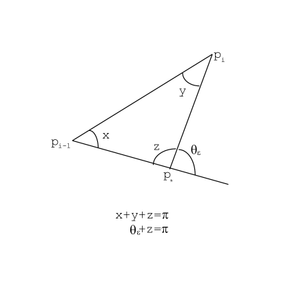
Figure 9. A classical fact of Euclidean geometry

This will allow us to handle the case of piecewise linear sets. Therefore the following corollary will be useful.

Corollary 3.7.

Let $S(\beta,\tau)$ be a set which can be expressed as

$$S=\bigl{\{}\,(x,y):x\in[a,b],\beta(x)\leq y\leq\tau(x)\,\bigr{\}}$$

where $\beta,\tau:[a,b]\rightarrow\mathbb{R}$ are piecewise $C^{2}$ functions such that

$$\beta(x)<\tau(x)_{,}\;\;\forall x\in(a,b).$$

Fix a spread $\sigma(\varepsilon)$ satisfying the conditions (3.1a) and (3.1b). For each $\varepsilon$ we choose compatible $\varepsilon$-upper/lower profiles $\Xi^{\pm}_{\varepsilon}$ of $S$ with common spread $\sigma(\varepsilon)$. We denote by ${S}_{\varepsilon}$ the $PL$ approximation of ${S}$ defined by these samples. Then

$$\lim_{\varepsilon\searrow 0}K(\partial S_{\varepsilon})=K(\partial S).$$

Proof.

Let

$$\Xi^{\pm}_{\varepsilon}=\bigl{\{}\xi_{0}^{\pm}\prec\xi_{1}^{\pm}\prec\cdots\prec\xi_{n}^{\pm}\,\bigr{\}},\;\;\xi_{k}^{\pm}=(x_{k}^{\pm},y_{k}^{\pm}).$$

The compatibility condition implies that

$$x_{k}^{-}=x_{k}^{+}=:x_{k},\;\;y_{k}^{-}\leq y_{k}^{+},\;\;\forall k=0,1,\dotsc,n.$$

Let $\beta_{\varepsilon}$ be the PL function whose graph is the bottom part of the boundary of $S_{\varepsilon}$, and $\tau_{\varepsilon}$ to be the PL function whose graph is the top part of the boundary of $S_{\varepsilon}$. Let $m_{i}^{\beta}(\varepsilon)$ indicate the slope of the $i$-th line segment of the graph of $\beta_{\varepsilon}$ and similarly let $m_{i}^{\tau}(\varepsilon)$ indicate the slope of the $i$-th line segment of the graph of $\tau_{\varepsilon}$. We have

$$\begin{split}K(\partial S_{\varepsilon})&=|\pi-\arctan(m_{1}^{\beta}(\varepsilon)\,)|\\ &+\sum_{i=2}^{n}|\arctan(m_{i}^{\beta}(\varepsilon)\,)-\arctan(m_{i-1}^{\beta}(\varepsilon)\,)|\\ &+|\arctan(m_{n}^{\beta}(\varepsilon))-\pi|+|\pi-\arctan(m_{1}^{\tau})|\\ &+\sum_{i=2}^{n}|\arctan(m_{i}^{\tau}(\varepsilon)\,)-\arctan(m_{i-1}^{\tau}(\varepsilon)\,)|\\ &+|\arctan(m_{n}^{\tau}(\varepsilon)\,)-\pi|\end{split}$$

which can be rewritten as

$$\begin{split}K(\partial S_{\varepsilon})&=|\pi-\arctan(m_{1}^{\beta}(\varepsilon)\,)|+|\arctan(m_{n}^{\beta}(\varepsilon)\,)-\pi|\\ &+|\pi-\arctan(m_{1}^{\tau}(\varepsilon)\,)|+|\arctan(m_{n}^{\tau}(\varepsilon)\,)-\pi|\\ &+K(\beta_{\varepsilon})+K(\tau_{\varepsilon})\end{split}$$ (3.13)

Proposition 3.6 implies

$$\lim_{\varepsilon\searrow 0}K(\beta_{\varepsilon})=K(\beta)\;\;\mbox{and}\;\;\lim_{\varepsilon\searrow 0}K(\tau_{\varepsilon})=K(\tau).$$ (3.14)

Now note that each line segment is defined by connecting two points in the pixelation of $\beta$ or $\tau$ over an interval of at most $\varepsilon\sigma(\varepsilon)$. Since as $\varepsilon\to 0$, $\varepsilon\sigma(\varepsilon)\to 0$, Theorem 2.6 implies that

$$\begin{split}\lim_{\varepsilon\searrow 0}m_{1}^{\beta}(\varepsilon)=\beta^{\prime}(a),\;\;\lim_{\varepsilon\searrow 0}m_{n}^{\beta}(\varepsilon)=\beta^{\prime}(b),\\ \lim_{\varepsilon\searrow 0}m_{1}^{\tau}(\varepsilon)=\tau^{\prime}(a),\;\;\lim_{\varepsilon\searrow 0}m_{n}^{\tau}(\varepsilon)=\beta^{\prime}(b).\end{split}$$ (3.15)

Combining (3.13), (3.14), (3.15) we find that

$$\begin{split}\lim_{\varepsilon\searrow 0}K(\partial S_{\varepsilon})&=|\pi-\arctan(\beta^{\prime}(a))|+|\arctan(\beta^{\prime}(b))-\pi|\\ &+|\pi-\arctan(\tau^{\prime}(a))|+|\arctan(\tau^{\prime}(b))-\pi|\\ &+K(\beta)+K(\tau).\end{split}$$ (3.16)

Note that $|\pi-\arctan(\beta^{\prime}(a))|$ is the value of the angle between the vertical line $x=a$ and the tangent line of $\beta$ at $a$. Similarly each other difference on the right hand side of (3.16) corresponds to an angle at one of the corners of $\partial S$. Therefore the right hand side of the (3.16) is equal to the $K(\partial S)$, so the corollary holds. $\hbox to0.0pt{$\sqcap$\hss}\sqcup$

4. Approximations of PL Sets and Morse Theory for Pixelations

In previous sections we have dealt only with the simple regions and we investigated mainly geometric properties of these regions and their pixelation. In this section we turn our attention to the relationship between the topology of a $PL$-set and those of its pixelations.

Surprisingly, this is a nontrivial matter. In general, the homotopy type of a region may not be not preserved when taking the pixelation. Worse, the homotopy type may never be recovered in any pixelation, even for small resolutions $\varepsilon$. This type of bad behavior can happen even for a simple PL case. Consider the set $S$ composed of the rays starting from the origin and proceeding in the positive direction with slopes $\frac{1}{2}$ and $\frac{1}{7}$ (see Figure 10). A careful examination of $P_{\varepsilon}(S)$ reveals the existence of cycle. Worse yet, the pixelations for smaller values of $\varepsilon$ are simply contractions of the larger pixelations. This means that $P_{\varepsilon}(S)$ contains a cycle for all small $\varepsilon$. For a taste of how much worse can this get we refer to Appendix A.

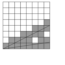
Figure 10. The pixelation of the lines with slope $\frac{1}{2}$ and $\frac{1}{7}$. After this point the pixelations of the upper and lower lines diverge permanently and no more holes are formed.

First, some good news. The next two results imply that if two compact planar sets are disjoint, then their pixelations will also be disjoint for sufficiently fine resolutions.

Theorem 4.1.

Let $S\subset\mathbb{R}^{2}$ be a compact set and let $x\in\mathbb{R}^{2}$ such that $x\notin S$. Set

$$m:=\inf_{s\in S}d(x,s),$$

where $d(\bullet,\bullet)$ is the Euclidean metric on $\mathbb{R}^{2}$, so that $m$ is the Hausdorff distance from $x$ to $S$. Then $\forall\varepsilon<\frac{m}{3}$, $x\notin P_{\varepsilon}(S)$.

Proof.

For $x$ to lie in $P_{\varepsilon}(S)$, both $x$ and a point of $S$ must lie in the same pixel. However the furthest two points can be apart in a square of side length $\varepsilon$ is $\varepsilon\sqrt{2}$ (if they lie on opposite corners of the square.) But since $\varepsilon<\frac{m}{3}$, $\varepsilon\sqrt{2}<\frac{m\sqrt{2}}{3}<m$, so it is impossible for a point of $S$ to lie in the same pixel as $x$. Therefore $x\notin P_{\varepsilon}(S)$. $\hbox to0.0pt{$\sqcap$\hss}\sqcup$

Corollary 4.2.

Let $S\subset\mathbb{R}^{2}$ be a compact set with finitely many connected components. Then for sufficiently small $\varepsilon$, the number of connected components of $P_{\varepsilon}(S)$ agrees with the number of connected components of $S$.

Proof.

First note that $P_{\varepsilon}(S)$ cannot have more connected components than $S$, since $P_{\varepsilon}(S)$ contains only pixels that intersect $S$.

Since $S$ is compact with finitely many components, there is a minimum positive distance $\delta$ between components. For each component $K$ of $S$ define

$$T_{K}:=\{x\in\mathbb{R}^{2}:\inf_{k\in K}d(x,k)\leq\frac{\delta}{2}\}$$

and note that its topological boundary is

$$\partial_{\mathrm{top}}T_{K}=\{x\in\mathbb{R}^{2}:\inf_{k\in K}d(x,k)=\frac{\delta}{2}\}$$

Then each point in $\partial T_{K}$ is $\frac{\delta}{2}$ away from $K$ in the Hausdorff metric. Furthermore, since $\delta$ is the minimum distance between components of $S$, each point in $\partial T_{K}$ is at least $\frac{\delta}{2}$ away from any connected component. Therefore, for $\varepsilon<\frac{\delta}{6}$ we have for each $K$

$$\partial T_{K}\cap P_{\varepsilon}(S)=\emptyset$$

This implies that for sufficiently small $\varepsilon$ each connected component of $P_{\varepsilon}(S)$ intersects at most one connected component of $S$. However, since

$$S\subset P_{\varepsilon}(S)$$

it is also true that each connected component of $S$ is contained within one connected component of $P_{\varepsilon}(S)$. Therefore for sufficiently small $\varepsilon$, $P_{\varepsilon}(S)$ and $S$ have the same number of connected components. $\hbox to0.0pt{$\sqcap$\hss}\sqcup$

The corollary guarantees that the zeroth Betti number of a set coincides with those of its sufficiently fine pixelations. Theorem 4.1 also suggests that, for small $\varepsilon$, the only way that the topological type of $P_{\varepsilon}(S)$ can disagree with that of $S$ is if $P_{\varepsilon}(S)$ has additional cycles (since every “real” cycle will show up in the pixelation). We will refer to these cycles as holes. More formally the holes are cycles in $P_{\varepsilon}(S)$ that are not contained in the image of the inclusion induced morphismlations. Theorem 4.1 also suggests that, for small $\varepsilon$, the only way that the topological type of $P_{\varepsilon}(S)$ can disagree with that of $S$ is if $P_{\varepsilon}(S)$ has additional cycles (since every “real” cycle will show up in the pixelation). We will refer to these cycles as holes. More formally the holes are cycles in $P_{\varepsilon}(S)$ that are not contained in the image of the inclusion induced morphism

$$H_{1}(S,\mathbb{Z})\rightarrow H_{1}\bigl{(}\,P_{\varepsilon}(S),\mathbb{Z}\,\bigr{)}.$$

Thus recovery of $S$ from $P_{\varepsilon}(S)$ will depend on distinguishing the cycles of $P_{\varepsilon}(S)$ that correspond to real cycles from $S$ from those that are merely artifacts of the pixelation. To discard these holes, we adopt a strategy inspired from Morse theory.

Definition 4.3.

Let $S\subset\mathbb{R}^{2}$ be a compact set and $\varepsilon>0$

1. For every $\varepsilon$-generic $x$ we set

   $$\boldsymbol{n}_{\varepsilon}(x)=\boldsymbol{n}_{S,\varepsilon}:=\#\text{ of connected components of }C_{\varepsilon}(S,x).$$

   (When the set $S$ is understood from context we use the simpler notation $\boldsymbol{n}_{\varepsilon}$ instead of $\boldsymbol{n}_{S,\varepsilon}$.) We will refer to $\boldsymbol{n}_{\varepsilon}(x)$ as the stack counter function of $S$.

2. We define

   $$\boldsymbol{n}(x)=\boldsymbol{n}_{S}(x):=\#\text{ of components of }\bigl{\{}\,y\in\mathbb{R};\;\;(x,y)\in S\,\bigr{\}}.$$

   We will refer to $\boldsymbol{n}_{S}(x)$ the component counter of $S$.

3. A jumping point of $\boldsymbol{n}_{S}$ is a real number $x_{0}$ such that

   $$\boldsymbol{n}(x_{0})\neq\boldsymbol{n}(x_{0}^{-}):=\lim_{x\nearrow x_{0}}\boldsymbol{n}(x)\;\;\mbox{or}\;\;\boldsymbol{n}(x)\neq\boldsymbol{n}(x_{0}^{+}):=\lim_{x\searrow x_{0}}\boldsymbol{n}(x).$$

   We denote by $\mathcal{J}_{S}$ the set of jumping points of $\boldsymbol{n}_{S}$. We will refer to $\mathcal{J}_{S}$ as the jumping set of $S$.

4. A jumping point of $\boldsymbol{n}_{\varepsilon}$ is a real number $x_{0}\in\varepsilon\mathbb{Z}$ such that

   $$\boldsymbol{n}_{\varepsilon}(x_{0}^{-})\neq\boldsymbol{n}(x_{0}^{+}).$$

   We denote by $\mathcal{J}_{S,\varepsilon}$ the set of jumping points of $\boldsymbol{n}_{S,\varepsilon}$. We will refer to it as the $\varepsilon$-jumping set of $S$.

$\hbox to0.0pt{$\sqcap$\hss}\sqcup$

The function $\boldsymbol{n}_{\varepsilon}$ tells us how many stacks are in a column. A cycle has two “walls” and a “gap.” That is to say, if there is a hole in $P_{\varepsilon}(S)$, there will be a set of columns which have more components than their neighbors, since for a hole to close up stacks must overlap. Thus jumps of $\boldsymbol{n}_{\varepsilon}$ are a first indicator of the presence of cycles in $P_{\varepsilon}(S)$. To decide whether they are holes, as opposed to cycles coming from $S$ we will rely on our next key technical result which is a substantial refinement of Theorem 4.1.

Theorem 4.4 (Separation Theorem).

Let $f,g:[a,b]\rightarrow\mathbb{R}$ be two Lipschitz continuous functions such that $f(x)\leq g(x)$, $\forall x\in[a,b]$. Fix $\varepsilon>0$ and suppose that $\exists x_{0}\in[a,b]$ such that

$$g(x_{0})-f(x_{0})\leq g(x)-f(x),\;\;\forall x\in[a,b],$$ (4.1)

Then for any $\varepsilon>0$ such that

$$\bigl{(}\,3+\min(\|f^{\prime}\|_{\infty},\|g^{\prime}\|_{\infty})\,\bigr{)}\varepsilon\leq g(x_{0})-f(x_{0})$$ (4.2)

and any $\varepsilon$-generic $x\in[a,b]\setminus\varepsilon\mathbb{Z}$ the column $C_{\varepsilon}(G,x)$ has two components. In other words, if

$$\min_{x\in[a,b]}\bigl{(}\,g(x)-f(x)\,\bigr{)}\geq\bigl{(}\,3+\min(\|f^{\prime}\|_{\infty},\|g^{\prime}\|_{\infty})\,\bigr{)}\varepsilon,$$

then for any $\varepsilon$-generic $x\in[a,b]$ we have

$$\boldsymbol{n}_{G,\varepsilon}(x)=\boldsymbol{n}_{G}(x).$$

Proof.

Note that

$$C_{\varepsilon}(G,x)=C_{\varepsilon}(f,x)\cup C_{\varepsilon}(g,x),$$

and furthermore, Theorem 2.2 implies that each of these columns is connected. Therefore $C_{\varepsilon}(G,x)$ will have two components only if $C_{\varepsilon}(f,x)$ and $C_{\varepsilon}(g,x)$ do not intersect. Since $f\leq g$ and $x$ is $\varepsilon$-generic, this will occur when

$$T_{\varepsilon}(f,x)<B_{\varepsilon}(g,x)$$

or equivalently,

$$B_{\varepsilon}(g,x)-T_{\varepsilon}(f,x)\geq\varepsilon$$

Now fix $x\in[a,b]$ and let $i\in\mathbb{Z}$ such that $i\varepsilon<x<(i+1)\varepsilon$. Choose $x_{f},x_{g}\in[i\varepsilon,(i+1)\varepsilon)]$ such that

$$f(x_{f})=\max_{x\in[i\varepsilon,(i+1)\varepsilon]}f(x),\;\;g(x_{g})=\min_{x\in[i\varepsilon,(i+1)\varepsilon]}g(x).$$

Therefore we have

$$B_{\varepsilon}(g,x)\geq g(x_{g})-\varepsilon,\;\;T_{\varepsilon}(f,x)\leq f(\,x_{f}\,)+\varepsilon,$$

so that

$$B_{\varepsilon}(g,x)-T_{\varepsilon}(f,x)\geq g(x_{g})-f(x_{f})-2\varepsilon.$$

We distinguish two cases.

Case 1. $\|g^{\prime}\|_{\infty}\leq\|f^{\prime}\|_{\infty}$. We have

$$B_{\varepsilon}(g,x)-T_{\varepsilon}(f,x)=g(x_{g})-g(x_{f})+g(\,x_{f}\,)-f(\,x_{f}\,)-2\varepsilon$$

$$\stackrel{{\scriptstyle(\ref{eq: gap0})}}{{\geq}}g(x_{g})-g(x_{f})+g(x_{0})-f(x_{0})-2\varepsilon$$

$$\geq g(x_{0})-f(x_{0})-\varepsilon\bigl{(}\,2+\|g^{\prime}\|_{\infty}\,\bigr{)}\stackrel{{\scriptstyle(\ref{eq: gap1})}}{{\geq}}\varepsilon.$$

Case 2. $\|f^{\prime}\|_{\infty}\leq\|g^{\prime}\|_{\infty}$. We have

$$B_{\varepsilon}(g,x)-T_{\varepsilon}(f,x)=g(x_{g})-f(x_{g})+f(\,x_{g}\,)-f(\,x_{f}\,)-2\varepsilon$$

$$\stackrel{{\scriptstyle(\ref{eq: gap0})}}{{\geq}}g(x_{0})-f(x_{0})+f(x_{g})-f(x_{f})-2\varepsilon$$

$$\geq g(x_{0})-f(x_{0})-\varepsilon\bigl{(}\,2+\|f^{\prime}\|_{\infty}\,\bigr{)}\stackrel{{\scriptstyle(\ref{eq: gap1})}}{{\geq}}\varepsilon.$$

$\hbox to0.0pt{$\sqcap$\hss}\sqcup$

To proceed further we need to introduce some basic terminology.

We define a convex polygon to be a compact set in $\mathbb{R}^{2}$ that is the intersection of finitely many closed half-planes. Note that points, and straight line segments are examples of convex polygons. A $PL$ set in $\mathbb{R}^{2}$ is a finite union of convex polygons. Note that the topological boundary of a $PL$ set is a finite union of straight line segments and points. A vertex of a $PL$ set $S$ is a point $p$ on the topological boundary $\partial_{\mathrm{top}}S$ of $S$ such that, for all $r>0$ sufficiently small, the intersection of $\partial_{\mathrm{top}}S$ with the closed ball of radius $r$ and center $p$ is not a straight line segment. We denote by $\mathcal{V}_{S}$ the set of vertices of a $PL$-set $S$.

Definition 4.5.

1. A convex polygon is a compact subset of $\mathbb{R}^{2}$ which is the intersection of finitely many closed half-planes (note that line segments and points are examples of convex polygons).

2. A $PL$ set (or piecewise linear set) in $\mathbb{R}^{2}$ is a finite union of convex polygons.

3. A vertex of a $PL$ set $S$ is a point $p$ on the topological boundary $\partial_{\mathrm{top}}S$ such that for all sufficiently small $r>0$, the intersection of $\partial_{\mathrm{top}}S$ with the closed ball of radius $r$ and center $p$ is not a straight line segments.

4. For a $PL$ set $S\subset\mathbb{R}^{2}$, the set of vertices $eV_{S}$ is the collection of all vertices in $S$.

5. A $PL$ subset in $S\subset\mathbb{R}^{2}$ is called generic if for any two vertices $p_{1},p_{2}\in\mathcal{V}_{S}$

   $$x(p_{1})\neq x(p_{2}).$$

$\hbox to0.0pt{$\sqcap$\hss}\sqcup$

We will restrict our approximation technique to the $PL$ case in order to simplify the conclusion of Theorem 4.4. Since our technique for determining holes will be motivated by applying Morse theory to projection onto the $x$-axis, we will also require the $PL$ set to be generic (to avoid complications arising from clusters of critical points sharing the same critical value). Note that for a $PL$ set $S$, the set of jumping points is contained in the set of $x$-coordinates of the vertices of $S$, that is

$$\mathcal{J}_{S}\subset\bigl{\{}x(p);\;\;p\in\mathcal{V}_{S}\,\bigr{\}}.$$

This inclusion could be strict. Take for example a $V$-shaped set, with the bottom vertex of the letter $V$ situated at the origin. Then $0$ is not a jumping point of $\boldsymbol{n}$.

Theorem 4.6.

Let $S$ be a generic $PL$ set with jumping set $\mathcal{J}_{S}$. Then there exist $\nu=\nu(S)\in\mathbb{Z}_{>0}$ and $\varepsilon_{0}=\varepsilon_{0}(S)>0$, depending only on $S$, such that, if $0<\varepsilon<\varepsilon_{0}$ and $x$ is an $\varepsilon$-generic value such that

$$\operatorname{dist}(x,\mathcal{J}_{S})\geq\nu\varepsilon,$$

then $\boldsymbol{n}_{S,\varepsilon}(x)=\boldsymbol{n}_{S}(x)$.

Proof.

Let $x_{0}<x_{1}<\cdots<x_{\ell}$ be the jumping points of $\boldsymbol{n}=\boldsymbol{n}_{S}$. We set

$$\Delta x_{i}:=x_{i}-x_{i-1},\;\;\forall i=1,\dotsc,\ell,\;\;\Delta:=\min_{1\leq i\leq\ell}\Delta x_{i}.$$

Note that $\boldsymbol{n}(x)$ is constant on each of the intervals $(x_{i-1},x_{i})$. For $i=1,\dotsc,\ell$ we set

$$S_{i}:=\bigl{\{}(x,y)\in S;\;\;x\in[x_{i-1},x_{i}]\,\bigr{\}}.$$

The set $S_{i}$ is a disjoint union of elementary sets (see Definition 3.1 for notations)

$$S(\beta_{i,j},\tau_{i,j}),\;\;j=0,\dots,p_{i},$$

“stacked one above the other”, i.e.,

$$\beta_{i,0}(x)\leq\tau_{i,0}(x)<\beta_{i,1}(x)\leq\tau_{i,1}(x)<\cdots<\beta_{i,p_{i}}(x)\leq\tau_{i,p_{i}}(x),\;\;\forall x\in(x_{i-1},x_{i}).$$ (4.3)

From Proposition 3.2 we deduce that for any $\varepsilon$-generic $x\in(x_{i-1},x_{i})$ we have $\boldsymbol{n}(x)=p_{i}$.

Each of the functions $\beta_{i,j}$ and $\tau_{i,j}$ is piecewise linear. Let $r_{i,j}$ be the smallest width of a line segment of the graphs $\beta_{i,j}$ and $\tau_{i,j}$, and we set

$$r_{i}:=\frac{1}{3}\min_{0\leq j\leq p_{i}}r_{i,j}.$$ (4.4)

By definition, $r_{i}\leq\frac{1}{3}\Delta x_{i}$. We set

$$S[x_{i-1}+r_{i},x_{i}-r_{i}]:=\bigl{\{}\,(x,y)\in S;\;\;x\in[x_{i-1}+r_{i},x_{i}-r_{i}]\,\bigr{\}}.$$

The set $S[x_{i-1}+r_{i-1},x_{i}-r_{i}]$ is a collection of $p_{i}$ elementary sets stacked one above the other which have positive Hausdorff distance between them. Theorem 4.1 implies that there exists $\delta_{i}>0$ such that, for $\varepsilon\in(0,\delta_{i})$ the pixelation $P_{\varepsilon}\bigl{(}\,S[x_{i-1}+r,x_{i}-r_{i}]\,\bigr{)}$ has exactly $p_{i}$ components. Therefore we have proven that

$$\exists\delta_{i}>0\;\;\mbox{such that};\;\forall\varepsilon\in(0,\delta_{i})\;\;x\in[x_{i-1}+r_{i},x_{i}-r_{i}]:\;\;\boldsymbol{n}(x)=\boldsymbol{n}_{\varepsilon}(x).$$ (4.5)

Set

$$y_{i}:=x_{i-1}+r_{i},\;\;z_{i}:=x_{i}-r_{i}.$$

On the interval $[x_{i-1},y_{i}]$ each of the functions $\beta_{i,j}$ and $\tau_{i,j}$ is linear and we denote by $m^{-}(\beta_{i,j})$ and respectively $m^{-}(\tau_{i,j})$ their slopes. For each $x\in(x_{i-1},x_{i})$ and each $j=1,\dotsc,p_{i}$ we define the gaps

$$\gamma_{i,j}(x)=\beta_{i,j}(x)-\tau_{i,j-1}(x),\;\;\gamma_{i,j}:=\min\bigl{\{}\gamma_{i,j}(x_{i-1}),\gamma_{j}(y_{i})\bigr{\}}=\min_{x\in[x_{i-1},y_{i}]}\gamma_{i,j}(x),$$

$$\Gamma_{i,j}:=\max\bigl{\{}\gamma_{i,j}(x_{i-1}),\gamma_{i,j}(y_{i})\bigr{\}}=\max_{x\in[x_{i-1},y_{i}]}\gamma_{i,j}(x).$$

We plan to invoke the Separation Theorem 4.4. We want to prove that there exists $\varepsilon_{0}>0$ and $\nu>0$ such that for $\varepsilon<\varepsilon_{0}$ we have

$$\min\bigl{\{}\gamma_{i,j}(x);\;x_{i-1}+\nu\varepsilon\leq x\leq y_{i}-\nu\varepsilon\,\bigr{\}}\geq\Bigl{(}\,3+\min\bigl{(}\,|m^{-}(\beta_{i,j})|,|m^{-}(\tau_{i,j-1})|\,\bigl{)}\,\Bigr{)}\varepsilon.$$ (4.6)

Note that if $2\nu\varepsilon<\Delta x_{i}$, then

$$\min\bigl{\{}\gamma_{i,j}(x);\;x_{i-1}+\nu\varepsilon\leq x\leq y_{i}-\nu\varepsilon\,\bigr{\}}=\gamma_{i,j}+\nu|m^{-}(\beta_{i,j})-m^{-}(\tau_{i,j-1})|\varepsilon.$$

We can now rewrite (4.6) as

$$\gamma_{i,j}\geq\Bigl{(}\,3+\min\bigl{(}\,|m^{-}(\beta_{i,j})|,|m^{-}(\tau_{i,j-1})|\,\bigl{)}-\nu|m^{-}(\beta_{i,j})-m^{-}(\tau_{i,j-1})|\,\Bigr{)}\varepsilon.$$ (4.7)

To solve the last inequality we distinguish two cases.

Case 1. $\gamma_{i,j}=0$. In this case the slope of $\beta_{i,j}$ must be different from the slope of $\tau_{i,j-1}$ and we choose $\nu=\nu^{-}_{i,j}$ large enough so that

$$3+\min\bigl{(}\,|m^{-}(\beta_{i,j})|,|m^{-}(\tau_{i,j-1})|\,\bigl{)}-\nu|m^{-}(\beta_{i,j})-m^{-}(\tau_{i,j-1})|<0,$$

e.g.,

$$\nu^{-}_{i,j}=\left\lfloor\frac{3+\min\bigl{(}\,|m^{-}(\beta_{i,j})|,|m^{-}(\tau_{i,j-1})|\,\bigl{)}}{|m^{-}(\beta_{i,j})-m^{-}(\tau_{i,j-1})|}\right\rfloor+1.$$

We then choose $\varepsilon^{-}(i,j)$ small enough such that $2\nu_{i,j}\varepsilon_{0}<\Delta x_{i}$, e.g.,

$$\varepsilon^{-}_{0}(i,j)=\frac{\Delta}{10\nu_{i,j}}.$$

Case 2. $\gamma_{i,j}\neq 0$. In this case we choose $\varepsilon_{0}=\varepsilon_{0}(i,j)$ small enough such that

$$\gamma_{i,j}>\Bigl{(}\,3+\min\bigl{(}\,|m^{-}(\beta_{i,j})|,|m^{-}(\tau_{i,j-1})|\,\bigl{)}\,\Bigr{)}\varepsilon_{0},$$

e.g.,

$$\varepsilon^{-}_{0}(i,j)=\frac{\gamma_{i,j}}{2\Bigl{(}\,3+\min\bigl{(}\,|m^{-}(\beta_{i,j})|,|m(\tau_{i,j-1})|\,\bigl{)}\,\Bigr{)}},$$

Next we choose $\nu=\nu^{-}_{i,j}$ such that $2\nu\varepsilon_{0}<\Delta x_{i}$, e.g.,

$$\nu^{-}_{i,j}=\left\lfloor\frac{\Delta}{10\varepsilon_{0}(i,j)}\right\rfloor.$$

Finally, we define set

$$\varepsilon_{i}^{-}:=\min_{0\leq j\leq p_{i}}\varepsilon^{-}(i,j),\;\;\nu_{i}^{-}=\max_{0\leq j\leq p_{i}}\nu^{-}_{i,j}.$$

Theorem 4.4 implies

$$\exists\varepsilon_{i}^{-}>0,\;\;\nu_{i}^{-}>0\;\;\mbox{such that}\;\;\forall\varepsilon<\varepsilon_{i}^{-},\;\;\forall x\in[x_{i-1}+\nu_{i}^{-}\varepsilon,x_{i-1}+r_{i}]:\;\;\boldsymbol{n}(x)=\boldsymbol{n}_{\varepsilon}(x).$$ (4.8)

Arguing in a similar fashion we deduce

$$\exists\varepsilon_{i}^{+}>0,\;\;\nu_{i}^{+}>0\;\;\mbox{such that}\;\;\forall\varepsilon<\varepsilon_{i}^{+},\;\;\forall x\in[x_{i}-r_{i},x_{i}-\nu_{i}^{+}\varepsilon]:\;\;\boldsymbol{n}(x)=\boldsymbol{n}_{\varepsilon}(x).$$ (4.9)

Now set

$$\nu_{i}:=\max(\nu_{i}^{-},\nu_{i}^{+}),\;\;\nu:=\max_{1\leq i\leq\ell}\nu_{i},$$

$$\varepsilon_{i}:=\min(\varepsilon_{i}^{-},\varepsilon_{i}^{+},\delta_{i}),\;\;\varepsilon_{0}=\min_{1\leq i\leq\ell}\varepsilon_{i}.$$

Theorem 4.6 now follows from (4.5), (4.8) and (4.9). $\hbox to0.0pt{$\sqcap$\hss}\sqcup$

This theorem tells us that jumps of $\boldsymbol{n}_{\varepsilon}$ occur within $\nu(S)$ pixels from the jumps in $\boldsymbol{n}$. A priori, it could be possible that, given a jumping point $x_{0}$ of $\boldsymbol{n}$, there is no jump in $\boldsymbol{n}_{\varepsilon}$ within $\nu(S)$ pixels of $x_{0}$.

Theorem 4.7.

Let $S$ be a generic PL set, and $\varepsilon_{0}=\varepsilon_{0}(S)$, $\nu=\nu(S)$ as in Theorem 4.6. Then, there exists $\varepsilon_{1}=\varepsilon_{1}(S)$ such that if $\varepsilon<\min(\varepsilon_{0},\varepsilon_{1})$ and $x_{0}$ is a jumping point of $\boldsymbol{n}=\boldsymbol{n}_{S}$, then $\boldsymbol{n}_{\varepsilon}=\boldsymbol{n}_{S,\varepsilon}$ has at least one jumping point in the interval $[x_{0}-\nu\varepsilon,x_{0}+\nu\varepsilon]$.

Proof.

Since $x_{0}$ is a jumping point of $\boldsymbol{n}$ we have

$$\boldsymbol{n}(x_{0}^{+})\neq\boldsymbol{n}(x_{0})\;\;\mbox{or}\;\;\boldsymbol{n}(x_{0})\neq\boldsymbol{n}(x_{0}^{-}).$$

We distinguish several cases cases.

Case 1. $\boldsymbol{n}(x_{0}^{-})>\boldsymbol{n}(x_{0})$. Since $S$ is compact, $\boldsymbol{n}(x_{0})>0$ so that $\boldsymbol{n}(x_{0}^{-})\geq 2$. For this to happen the vertical line of $x=x_{0}$ must contain at least one vertex of $S$. Since $S$ is generic, this line contains precisely one vertex of $S$, which we denote by $p_{0}$.

We can find $\delta>0$ sufficiently small such that the interval $[x_{0}-\delta,x_{0}]$ will contain no new jumping points of $S$. The set

$$S_{[x_{0}-\delta,x_{0}]}:=\bigl{\{}(x,y)\in S;\;\;x\in[x_{0}-\delta,x_{0}]\,\bigr{\}}$$

is disjoint union of simple types regions

$$S(\beta_{j},\tau_{j}),\;\;j=0,\dots,m=\boldsymbol{n}(x_{0}^{-})-1,$$

“stacked one above the other”, i.e.,

$$\beta_{0}(x)\leq\tau_{0}(x)<\beta_{1}(x)\leq\tau_{1}(x)<\cdots<\beta_{m}(x)\leq\tau_{m}(x),\;\;\forall x\in(x_{0}-\delta,x_{0}),$$

where $\beta_{j},\tau_{j}$ are piecewise linear functions. Since $\boldsymbol{n}(x_{0})<\boldsymbol{n}(x_{0}^{-})$ we deduce that there exists $j_{0}=1,\dotsc,m$ such that

$$\beta_{j_{0}}(x_{0})=\tau_{j_{0}-1}(x_{0})\;\;\mbox{and}\;\;\gamma_{j}:=\beta_{j}(x_{0})-\tau_{j-1}(x_{0})>0,\;\;\forall j\neq j_{0}$$

In particular, for any $\varepsilon>0$, the $\varepsilon$-stack of $S(\beta_{j_{0}},\tau_{j_{0}})$ over $x_{0}$ touches the stack of $S(\beta_{j_{0}-1},\tau_{j_{0}-1})$ over $x_{0}$.

Now choose $\varepsilon_{1}$ sufficiently small so that for $j\neq j_{0}$ and $\varepsilon<\varepsilon_{1}$, the $\varepsilon$-stack of $S(\beta_{j},\tau_{j})$ over $x_{0}$ is disjoint form the $\varepsilon$-stack of $S(\beta_{j-1},\tau_{j-1})$ over $x_{0}$. Fix $\varepsilon<\min(\varepsilon_{0},\varepsilon_{1})$. The above discussion shows that

$$\boldsymbol{n}(x_{0})=\boldsymbol{n}_{\varepsilon}(x_{0}^{-}).$$

Theorem 4.6 now implies that

$$\boldsymbol{n}_{\varepsilon}((x_{0}-\nu\varepsilon)^{-})=\boldsymbol{n}(x_{0}-\nu\varepsilon)>\boldsymbol{n}(x_{0}).$$

This proves that the interval $[x_{0}-r\varepsilon,x_{0}]$ contains a jumping point of $\boldsymbol{n}_{\varepsilon}$.

Case 2. $\boldsymbol{n}(x_{0}^{+})>\boldsymbol{n}(x_{0})$. This situation can be reduced to the previous case via the reflection

$$\mathbb{R}^{2}\ni(x,y)\mapsto(-x,y)\in\mathbb{R}^{2}.$$

Case 3. $\boldsymbol{n}(x_{0}^{-})<\boldsymbol{n}(x_{0})$. The vertical line $x=x_{0}$ contains a unique vertex $p_{0}$ of $S$. Moreover, this vertex has the property that there exists a tiny disk $D$ centered at $p_{0}$ such that the intersection of $D$ with the open half-plane $\{x<x_{0}\}\subset\mathbb{R}^{2}$ is empty. In particular, this shows that $p_{0}$ is an isolated point of the set

$$S_{x\leq x_{0}}=\bigl{\{}(x,y)\in S;\;\;x\leq x_{0}\,\bigr{\}}.$$

If $\boldsymbol{n}(x_{0}^{-})=0$, the conclusion is obvious. We assume that $\boldsymbol{n}(x_{0}^{-})>0$. Choose $\delta>0$ such that the interval $[x_{0}-\delta,x_{0})$ contains no jumping point of $S$. Set

$$R:=S_{[x_{0}-\delta,x_{0}]}\setminus\{p_{0}\}.$$

Then $R$ is a union of simple regions

$$S(\beta_{,}\tau_{j}),\;\;j=0,1\dotsc,m=\boldsymbol{n}(x_{0}^{-})-1,$$

where $\beta_{j}$ and $\tau_{j}$ are piecewise linear functions such that

$$\beta_{0}(x)\leq\tau_{0}(x)<\beta_{1}(x)\leq\tau_{1}(x)<\cdots<\beta_{m}(x)\leq\tau_{m}(x),\;\;\forall x\in[x_{0}-\delta,x_{0}].$$

We can find $\varepsilon_{1}=\varepsilon_{1}(S)$ such that for any $\varepsilon<\varepsilon_{1}$ and any $\varepsilon$-generic $x\in[x_{0}-\delta,x_{0}]$ we have:

• $\boldsymbol{n}_{R,\varepsilon}(x)=\boldsymbol{n}_{S}(x)=m+1=\boldsymbol{n}_{S}(x_{0}^{-})$, and

• the $\varepsilon$-column of $S_{[x_{0}-\delta,x_{0}]}$ over $x_{0}$ consists of $\boldsymbol{n}(x_{0})=m+2$ stacks.

Theorem 4.6 implies that

$$\boldsymbol{n}_{S,\varepsilon}(x)=\boldsymbol{n}_{S}(x)=\boldsymbol{n}_{S}(x_{0}^{-})=m+1\;\;\forall x\in[x_{0}-\delta,x_{0}-\nu\varepsilon]\setminus\mathbb{Z}\varepsilon.$$

On the other hand, $\boldsymbol{n}_{S,\varepsilon}(x_{0}^{-})=m+2$. Thus the interval $[x_{0}-\nu\varepsilon,x_{0}]$ must contain a jumping point of $\boldsymbol{n}_{S,\varepsilon}$.

Case 4. $\boldsymbol{n}(x_{0}^{+})<\boldsymbol{n}(x_{0})$. This reduces the the previous case via the reflection

$$\mathbb{R}^{2}\ni(x,y)\mapsto(-x,y)\in\mathbb{R}^{2}.$$

$\hbox to0.0pt{$\sqcap$\hss}\sqcup$

Remark 4.8.

Theorem 4.6 states that the two functions $\boldsymbol{n}$ and $\boldsymbol{n}_{\varepsilon}$ coincide at points situated at a distance at least $\nu(S)$ pixels away from the jumping points of $\boldsymbol{n}$. On the other hand, Theorem 4.7 shows that, for a generic $PL$ set, within $\nu(S)$ pixels from a jumping point of $\boldsymbol{n}$ there must be jumping points of $\boldsymbol{n}_{\varepsilon}$. $\hbox to0.0pt{$\sqcap$\hss}\sqcup$

Definition 4.9.

Let $S$ be a generic $PL$ set in $\mathbb{R}^{2}$.

1. We will refer to the integer $\nu(S)$ as the noise range of $S$.

2. Let $\varepsilon_{0}(S)$ and $\varepsilon_{1}(S)$ as defined in the Theorems 4.6 and 4.7. We set

   $$\hbar(S):=\min\bigl{(}\,\varepsilon_{0}(S),\;\varepsilon_{1}(S)\,\bigr{)},$$

   and we will refer to it as the critical resolution of $S$.

$\hbox to0.0pt{$\sqcap$\hss}\sqcup$

The next result explains the roles of the noise range and the critical resolution.

Proposition 4.10.

Let $S$ be a generic PL set. If $w>2\nu(S)$, $\varepsilon<\hbar(S)$ and $[x_{0}-w\varepsilon,x_{0}+w\varepsilon]$ contains no jumping points of $\boldsymbol{n}_{\varepsilon}$, then $\boldsymbol{n}_{\varepsilon}(x_{0})=\boldsymbol{n}(x_{0})$.

Proof.

Suppose that the interval $[x_{0}-w\varepsilon,x_{0}+w\varepsilon]$ contains no jumping points of $\boldsymbol{n}_{\varepsilon}$, yet $\boldsymbol{n}_{\varepsilon}(x_{0})\neq\boldsymbol{n}(x_{0})$. Then Theorem 4.6 implies that the interval

$$[x_{0}-\frac{w}{2}\varepsilon,x_{0}+\frac{w}{2}\varepsilon]$$

contains a critical $x_{1}$ point of $\boldsymbol{n}$. Then Theorem 4.7 implies that $\boldsymbol{n}_{\varepsilon}$ has a jumping point on the interval

$$[x_{1}-\frac{w}{2}\varepsilon,x_{1}+\frac{w}{2}\varepsilon]$$

But since $x_{1}$ is at most $\frac{w}{2}$-pixels from $x_{0}$, this interval is contained within $[x_{0}-w\varepsilon,x_{0}+w\varepsilon]$. This contradicts the assumption that the interval contained no jumping points of $\boldsymbol{n}_{\varepsilon}$ and thus $\boldsymbol{n}_{\varepsilon}(x_{0})=\boldsymbol{n}(x_{0})$. $\hbox to0.0pt{$\sqcap$\hss}\sqcup$

Suppose that $\varepsilon<\hbar(S)$, where $S$ is a generic $PL$ set. Then the theorems proven in this section up to this point imply that all the jumping points of $\boldsymbol{n}_{\varepsilon}$ are contained a fixed numbers of pixels from the jumping set of $\boldsymbol{n}$. This simple observation, correctly implemented, will be the key to recovering the topology of $S$ from the topology of its sufficiently fine pixelations.

Consider the discontinuities of the function $\boldsymbol{n}_{\varepsilon}$. They can only occur within $\nu(S)$ columns from a jumping point of $\boldsymbol{n}$. We do not know what this integer is from the pixelation, but we know that it exists and it is independent of $\varepsilon$. Therefore, we know that the noise range $\nu(S)$ will eventually be less than a properly chosen spread $\sigma(\varepsilon)$ such that $\sigma(\varepsilon)\rightarrow\infty$ as $\varepsilon\rightarrow 0$. Using the spread to estimate $\nu(S)$ will be a dramatic overestimation for small $\varepsilon$. However since $\varepsilon\sigma(\varepsilon)\to 0$, if we declare any cycle which appears less than $\sigma(\varepsilon)$ columns from a jumping point of $n_{\varepsilon}(S)$ as a fake cycle, we will avoid declaring any real cycles as fake for small resolutions.

The discontinuities $\boldsymbol{n}_{\varepsilon}(S)$ (for sufficiently small $\varepsilon$) are obviously contained in the set

$$\{x\in\mathbb{R}:[x-\varepsilon\sigma(\varepsilon),x+\varepsilon\sigma(\varepsilon)]\text{ contains a critical value of }n_{\varepsilon}\}.$$

We would like to consider this set to be the “noise portion” of $S$. This would mean that we could approximate $S$ from $P_{\varepsilon}(S)$ over $x$-values outside of this region using the results from section 3. However, recall that in section 3 elementary sets were approximated by choosing upper and lower samples, which were chosen from the midpoints of pixels. This means that to use the methods from section 3 to approximate $S$ we need our noise intervals to end at the middle of a pixel. With that in mind we define the noise interval:

Definition 4.11.

Let $S$ be a generic $PL$ set, and let $x_{1},x_{2},\cdots,x_{N}$ be the jumping points of $\boldsymbol{n}_{S,\varepsilon}$. For each jumping point $x_{j}$ let the noise interval $I_{j}(\varepsilon)$ be the interval $[a_{j},b_{j}]$ where

$$x_{j}\in[a_{j},b_{j}],$$

$$a_{j}(\varepsilon),b_{j}(\varepsilon)\in\frac{\varepsilon}{2}+\varepsilon\mathbb{Z}$$

$$b_{j}\text{ is the smallest number in }\frac{\varepsilon}{2}+\varepsilon\mathbb{Z}\text{ such that }(b_{j}-x_{j})>2\varepsilon\sigma(\varepsilon)$$

$$a_{j}\text{ is the largest number in }\frac{\varepsilon}{2}+\varepsilon\mathbb{Z}\text{ such that }(x_{j}-b_{j})>2\varepsilon\sigma(\varepsilon)$$

Define the set of noise intervals $\Delta_{\varepsilon}$ as

$$\Delta_{\varepsilon}=I_{1}(\varepsilon)\cup\cdots\cup I_{N}(\varepsilon).$$

$\hbox to0.0pt{$\sqcap$\hss}\sqcup$

From the definition we see that $\Delta_{\varepsilon}$ is a union of intervals. Furthermore for small $\varepsilon$, each of these intervals will contain precisely one jumping point of $\boldsymbol{n}_{S}$. Thus $\Delta_{\varepsilon}(S)$ has as many components as the cardinality of $\mathcal{J}_{S}$. In particular this implies that the measure of $\Delta_{\varepsilon}$ is bounded from above by $2|\mathcal{J}_{S}|\varepsilon\sigma(\varepsilon)$. Since $\varepsilon\sigma(\varepsilon)$ vanishes as $\varepsilon\to 0$, this implies that $\Delta_{\varepsilon}$ has vanishing measure as $\varepsilon\to 0$.

Consider the set of $x$-values which lie outside the noise. It is a finite union of intervals such that for all $x$ which lie in these intervals, $\boldsymbol{n}_{\varepsilon}(x)=\boldsymbol{n}(x)$. The part of $S$ situated above a each interval is either empty, or a disjoint union of regions of simply types. These types of regions can be approximated using the methods described in Section 3. Therefore, to complete the approximation of $S$, we need only describe how to deal with the noise intervals.

The key observation is that the measure of $\Delta_{\varepsilon}$ goes to zero as $\varepsilon\to 0$ with the properly chosen spread. This means that noise intervals make up a very small part of $S$, and so it will not be necessary to approximate them with as high of degree of accuracy as other parts of $S$. Indeed, we only seek to ensure that the noise intervals capture the correct homotopy type for small values of $\varepsilon$.

Since $S$ is defined by a finite number of piecewise linear functions, for small enough $\varepsilon$, the part of $S$ above $\Delta_{\varepsilon}$ consists of contractible connected components. Theorem 4.1 implies that these components separate for small enough $\varepsilon$. Therefore the easiest way to get the correct topology within the noise intervals is to simply cover each component of the pixelation above a noise interval with a rectangle, destroying any fake cycles (or holes) from $P_{\varepsilon}(S)$ (see Figure 11.)

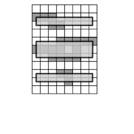
Figure 11. The approximation of a noise interval. The red rectangles indicate the rectangles that form the approximation. Since the intersection of a noise interval and a regular interval always lie on the centers of a column, the edges of the rectangles will intersect approximations from the regular intervals.

Suppose that $S$ is a generic $PL$ set with jump set

$$\mathcal{J}_{S}=\{x_{1}<\cdots<x_{N}\}.$$

We describe below an the algorithm to create a $PL$ approximation $S_{\varepsilon}$v for $S$ using only information from $P_{\varepsilon}(S)$ is as follows (this algorithm is restated in a more concrete way in Appendix D).

Algorithm 4.12.

1. Choose a spread $\sigma$ such that $\varepsilon\sigma(\varepsilon)^{2}\to\infty$ and $\varepsilon\sigma(\varepsilon)\to 0$ as $\varepsilon\to 0$.

2. Let $\Delta_{\varepsilon}$ be the noise intervals of $P_{\varepsilon}(S)$.

3. Define $\mathcal{R}_{\varepsilon}$ to be the closure of $\mathbb{R}\setminus\Delta_{\varepsilon}$. We call $\mathcal{R}_{\varepsilon}$ the regular set, and its intervals are called regular intervals.

4. For the bounded regular interval $I\in\mathcal{R}_{\varepsilon}$ do the following:

   1. For each connected component of $P_{\varepsilon}(S)\cap(I\times\mathbb{R})$, the part of $P_{\varepsilon}(S)$ over the regular regular intervals $I$ choose compatible upper and lower profiles $\Pi_{\varepsilon}^{+}$ and $\Pi_{\varepsilon}^{-}$ on that component.

   2. For each connected component, choose compatible upper and lower samples $\Xi_{\varepsilon}^{+}$ and $\Xi_{\varepsilon}^{-}$ with spread $\sigma$.

   3. For each connected component, take the PL approximation of the upper and lower samples.

   4. Add each PL approximation to the approximation of $S$.

5. For each regular point $x$ denote by $S_{\varepsilon}(x)$ the part of $S_{\varepsilon}$ over $x$, i.e.,

   $$S_{\varepsilon}(x):=S_{\varepsilon}\cap\{x\}\times\mathbb{R}.$$

6. For a noise interval $I_{j}(\varepsilon)$ we observe first that Corollary 4.2 implies that the number of connected components of $P_{\varepsilon}(S)$ over $I_{j}(\varepsilon)$ is equal to the number of components of $S$ over $I_{j}(\varepsilon)$. Denote by $\mathcal{C}_{j}(\varepsilon)$ the set of connected components of $P_{\varepsilon}(S)$ over $I_{j}(\varepsilon)$

   1. For every $C\in\mathcal{C}_{j}(\varepsilon)$ of $P_{\varepsilon}(S)$ we set

      $$U_{C}:=\max\{y;\;\;(x,y)\in C\,\bigr{\}},\;\;L_{C}:=\min\{y;\;\;(x,y)\in C\,\bigr{\}}.$$

   2. Let $P_{U}^{a}$ denote the pixel whose top boundary lies on the line $\{y=U_{C}\}$ and intersects the line $\{x=S_{\varepsilon}(a_{j}(\varepsilon))\}$. Similarly let $P_{U}^{b}$ denote the pixel whose top boundary lies on the line $\{y=U_{C}\}$ and intersects the line $\{x=S_{\varepsilon}(b_{j}(\varepsilon))\}$, let $P_{L}^{a}$ denote the pixel whose bottom boundary lies on the line $\{y=L_{C}\}$ and intersects the line $\{x=S_{\varepsilon}(a_{j}(\varepsilon))\}$ and $P_{L}^{b}$ denote the pixel whose bottom boundary lies on the line $\{y=L_{c}\}$ and intersects the line $\{x=S_{\varepsilon}(b_{j}(\varepsilon))\}$. (These pixels lie on the corners of a rectangle which bounds the majority of $C$, see Figure 11.)

   3. Let $U_{C}^{a}$ indicate the center of $P_{U}^{a}$ and similarly let $U_{C}^{b}$, $U_{L}^{a}$ and $U_{L}^{b}$ indicate the centers of $P_{U}^{b}$, $P_{L}^{a}$ and $P_{L}^{B}$.

   4. Denote by $\mathcal{P}_{C}(\varepsilon)$ the convex quadrilateral with vertices

      $$\begin{split}B_{j}^{-}(\varepsilon)=(b_{j}(\varepsilon),L_{C}^{b}),\;\;B_{j}^{+}(\varepsilon):=(b_{j}(\varepsilon),U_{C}^{b}),\\ A_{j}^{-}(\varepsilon)=(a_{j}(\varepsilon),L_{C}^{a}),\;\;A_{j}^{+}(\varepsilon):=(a_{j}(\varepsilon),U_{C}^{a})\end{split}$$

7. To the set $S_{\varepsilon}$ constructed at (4) add the noise union

   $$\mathcal{N}_{\varepsilon}:=\bigcup_{j=1}^{N}\bigcup_{C\in\mathcal{C}_{j}(\varepsilon)}\mathcal{P}_{C}(\varepsilon).$$

This final set $S_{\varepsilon}$ will be piecewise linear by construction, and will be a good approximation of the set. $\hbox to0.0pt{$\sqcap$\hss}\sqcup$

5. The Main Result

Consider a generic $PL$ subset $S$ of the Euclidean plane $\mathbb{E}=\mathbb{R}^{2}$. In section 4 we created Algorithm 4.12 which creates a $PL$ approximation $S_{\varepsilon}$ of $S$. We wish to state that this approximation converges in a good way to $S$. An appropriate language to state this condition is that of normal cycles.

For any compact $PL$ subset $X\subset\mathbb{E}$ we denote by $N^{X}$ its normal cycle, [7, 21]. For the reader’s convenience we have included in Appendix C a brief survey of the basic properties of the normal cycle. In particular Appendix C demonstrates how to recover both the Euler characteristic and the perimeter of a set using only calculations on the normal cycle. Using similar techniques we can extract other geometric and topological information about a set using only its normal cycle. Therefore weak convergence in normal cycles implies convergence of a great deal of important information, and is an appropriate condition for “good convergence.”

In the final theorem we see that the approximation $S_{\varepsilon}$ created by Algorithm 4.12 does satisfy this type of convergence.

Theorem 5.1.

Suppose $S$ is a generic $PL$ subset of $\mathbb{E}$, $\sigma(\varepsilon)$ is a spread function satisfying (3.1a) and $S_{\varepsilon}$ is the $PL$ approximation of $S$ constructed via the Algorithm 4.12. Then the normal cycle $N^{S_{\varepsilon}}$ of $S_{\varepsilon}$ converges weakly to the normal cycle $N^{S}$ of $S$.

Proof.

Let us first outline the strategy. Recall that $\mathcal{V}_{S}$ indicates the set of vertices of $S$ and denote by $\mathcal{X}_{S}$ its projection on the $x$-axis. Since $S$ is generic the projection $\mathbb{E}\ni(x,y)\mapsto x\in\mathbb{R}$ induces a bijection $\mathcal{V}_{S}\rightarrow\mathcal{X}_{S}$. The jump set $\mathcal{J}_{S}$ is contained in $\mathcal{X}_{S}$. We will refer to the vertices that project in $\mathcal{J}_{S}$ as essential vertices. The other vertices will be called inessential.

For every $c\in\mathcal{J}_{S}$ and any $\varepsilon>0$ small we denote by $I_{\varepsilon}(c)$ the noise interval that contains $c$. We set $I_{0}(c):=\{c\}$. Fix $\varepsilon_{0}>0$ such that,

$$\operatorname{dist}\bigl{(}\,\Delta_{\varepsilon}(c),\Delta_{\varepsilon}(c^{\prime})\,\bigr{)}\leq\frac{1}{4}\operatorname{dist}(c,c^{\prime}),\;\;\forall c,c^{\prime}\in\mathcal{J}_{S},\;\;0\leq\varepsilon\leq\varepsilon_{0}.$$

For $c\in\mathcal{J}_{S}$ and any $0\leq\varepsilon\leq\varepsilon_{0}$ we denote by $\mathcal{N}_{\varepsilon}(c)$ the noise strip

$$\mathcal{N}_{\varepsilon}(c):=\bigl{\{}\,(x,y)\in\mathbb{R}^{2};\;\;x\in I_{\varepsilon}(c)\,\bigr{\}}.$$

Note that $\mathcal{N}_{0}(c)$ is the vertical line $\{x=c\}$. Finally we set

$$\mathcal{N}_{\varepsilon}=\bigcup_{c\in\mathcal{J}_{S}}\mathcal{N}_{\varepsilon}(c),\;\;\mathcal{R}_{\varepsilon}:=\mathbb{R}^{2}\setminus\mathcal{N}_{\varepsilon},\;\;\forall 0\leq\varepsilon\leq\varepsilon_{0}.$$

For uniformity, we set $S_{0}:=S$.

Observe that there exists $0<\varepsilon_{1}<\varepsilon_{0}$ such that, if $\varepsilon\in[0,\varepsilon_{1}]$, the following hold.

• Any component of $\mathcal{N}_{0}\cap S_{0}$ is contained in a unique component of $\mathcal{N}_{\varepsilon}\cap S_{\varepsilon}$.

• If $C$ is a connected component of $\mathcal{R}_{\varepsilon}\cap S_{\varepsilon}$, then the closure of $C$ intersects exactly two connected components of $\mathcal{N}_{\varepsilon}\cap S_{\varepsilon}$.

For any $\varepsilon\in[0,\varepsilon_{1}]$ we construct a graph $\Gamma_{\varepsilon}$ as follows. The vertex set $\mathcal{V}_{\varepsilon}$ of $\Gamma_{\varepsilon}$ consists of the connected components of $\mathcal{N}_{\varepsilon}\cap S_{\varepsilon}$. The edges are the connected components of $\mathcal{R}_{\varepsilon}\cap S_{\varepsilon}$. We have a well defined map

$$\Psi_{\varepsilon}:\mathcal{V}_{0}\rightarrow\mathcal{V}_{\varepsilon},$$

that associates to the a component $C$ of $\mathcal{N}_{0}\cap S$ the unique component of $S_{\varepsilon}\cap\mathcal{N}_{\varepsilon}$ that contains $C$. which This is easily seen to be a bijection. Moreover, it induces an isomorphism of graphs, i.e., the vertices ${\boldsymbol{v}},{\boldsymbol{v}}^{\prime}$ are adjacent in $\Gamma_{0}$ if and only if the vertices $\Psi_{\varepsilon}({\boldsymbol{v}})$ and $\Psi_{\varepsilon}({\boldsymbol{v}}^{\prime})$ are adjacent in $\Gamma_{\varepsilon}$. For any ${\boldsymbol{v}}\in\mathcal{V}_{0}$ we denote by $E_{\boldsymbol{v}}$ the set of edges of $\Gamma_{0}$ that are adjacent to ${\boldsymbol{v}}$.

Remark 5.2.

The graph $\Gamma_{0}$ is known in the literature as the Reeb graph of the (stratified) Morse function

$$S\ni(x,y)\mapsto x\in\mathbb{R}.$$

For more information about this concept we refer to [4, VI.4], or the original source [22]. $\hbox to0.0pt{$\sqcap$\hss}\sqcup$

For any vertex ${\boldsymbol{v}}\in\mathcal{V}_{0}$ and $\varepsilon\in[0,\varepsilon_{1}]$ we denote by $C_{{\boldsymbol{v}},\varepsilon}$ the component of $\mathcal{N}_{\varepsilon}\cap S_{\varepsilon}$ corresponding to $\Psi_{\varepsilon}(v)$. Similarly, for any edge ${\boldsymbol{e}}=[{\boldsymbol{v}},{\boldsymbol{v}}^{\prime}]$ of $\Gamma_{0}$ and any $\varepsilon\in[0,\varepsilon_{1}]$ we denote by $C_{{\boldsymbol{e}},\varepsilon}$ the closure of the component of $\mathcal{R}_{\varepsilon}\cap S_{\varepsilon}$ corresponding to the edge $[\Psi_{\varepsilon}({\boldsymbol{v}}),\Psi_{\varepsilon}({\boldsymbol{v}}^{\prime})]$.

Lemma 5.3.

For any $\varepsilon\in[0,\varepsilon_{1}]$ we have

$$N^{S_{\varepsilon}}=\sum_{{\boldsymbol{v}}\in\mathcal{V}_{0}}N^{C_{{\boldsymbol{v}},\varepsilon}}+\sum_{{\boldsymbol{e}}\in\mathcal{E}_{0}}N^{C_{{\boldsymbol{e}},\varepsilon}}-\sum_{{\boldsymbol{v}}\in\mathcal{V}_{0}}\sum_{{\boldsymbol{e}}\in E_{\boldsymbol{v}}}N^{C_{{\boldsymbol{v}},\varepsilon}\cap C_{{\boldsymbol{e}},\varepsilon}}.$$ (5.1)

Proof.

The proof use the inclusion-exclusion principle, i.e., the equality

$$N^{X\cup Y}=N^{X}+N^{Y}-N^{X\cap Y}$$

for any compact $PL$ subsets $X,Y\subset\mathbb{R}^{2}$.

Note that we have a decomposition

$$S_{\varepsilon}=\left(\bigcup_{{\boldsymbol{v}}\in\mathcal{V}_{0}}C_{{\boldsymbol{v}},\varepsilon}\right)\cup\left(\bigcup_{{\boldsymbol{e}}\in\mathcal{E}_{0}}C_{{\boldsymbol{e}},\varepsilon}\right).$$ (5.2)

We need to discuss separately the cases $\varepsilon>0$ and $\varepsilon=0$.

1. Assume that $\varepsilon\in(0,\varepsilon_{1}]$. In this case we have

$$C_{{\boldsymbol{v}},\varepsilon}\cap C_{{\boldsymbol{v}}^{\prime},\varepsilon}=\emptyset=C_{{\boldsymbol{e}},\varepsilon}\cap C_{{\boldsymbol{e}}^{\prime},\varepsilon},\;\;\forall{\boldsymbol{v}}\neq{\boldsymbol{v}}^{\prime},\;\;{\boldsymbol{e}}\neq{\boldsymbol{e}}^{\prime}.$$ (5.3)

The equality (5.1) now follows from inclusion-exclusion principle applied to the decomposition (5.2) satisfying the overlap conditions (5.3).

2. Assume that $\varepsilon=0$. In this case the overlap conditions are more complicated. We have

$$C_{{\boldsymbol{v}},0}\cap C_{{\boldsymbol{v}}^{\prime},0}=\emptyset,\;\;\forall{\boldsymbol{v}}\neq{\boldsymbol{v}}^{\prime},$$ (5.4a)

$$C_{{\boldsymbol{e}},0}\cap C_{{\boldsymbol{e}}^{\prime},0}=\emptyset\Longleftrightarrow{\boldsymbol{e}}\cap{\boldsymbol{e}}^{\prime}=\emptyset,$$ (5.4b)

where the condition ${\boldsymbol{e}}\cap{\boldsymbol{e}}^{\prime}=\emptyset$ signifies that the edges ${\boldsymbol{e}}$ and ${\boldsymbol{e}}^{\prime}$ have no vertex in common. Moreover,

$$\bigcap_{{\boldsymbol{e}}\in A}C_{{\boldsymbol{e}},0}=C_{{\boldsymbol{v}},0},\;\;\forall{\boldsymbol{v}}\in\mathcal{V}_{0},\;\;A\subset E_{\boldsymbol{v}}.$$ (5.5)

Using (5.2), (5.4a), (5.4b), (5.5) and the inclusion-exclusion principle we deduce

$$\begin{split}N^{S}=&\sum_{{\boldsymbol{v}}\in\mathcal{V}_{0}}N^{C_{{\boldsymbol{v}},0}}+\sum_{{\boldsymbol{e}}\in\mathcal{E}_{0}}N^{C_{{\boldsymbol{e}},0}}-\sum_{{\boldsymbol{v}}\in\mathcal{V}_{0}}\sum_{{\boldsymbol{e}}\in E_{\boldsymbol{v}}}N^{C_{{\boldsymbol{v}},0}\cap C_{{\boldsymbol{e}},0}}\\ &+\sum_{{\boldsymbol{v}}\in\mathcal{V}_{0}}\sum_{\emptyset\neq A\subset E_{\boldsymbol{v}}}(-1)^{|A|+1}N^{C_{{\boldsymbol{v}}}\cap(\bigcap_{{\boldsymbol{e}}\in A})C_{{\boldsymbol{e}},0}}+\sum_{{\boldsymbol{v}}\in\mathcal{V}_{0}}\sum_{\emptyset\neq A\subset E_{\boldsymbol{v}}}(-1)^{|A|}N^{\bigcap_{{\boldsymbol{e}}\in A}C_{{\boldsymbol{e}},0}}\end{split}$$

$$\begin{split}&=\sum_{{\boldsymbol{v}}\in\mathcal{V}_{0}}N^{C_{{\boldsymbol{v}},0}}+\sum_{{\boldsymbol{e}}\in\mathcal{E}_{0}}N^{C_{{\boldsymbol{e}},0}}-\sum_{{\boldsymbol{v}}\in\mathcal{V}_{0}}\sum_{{\boldsymbol{e}}\in E_{\boldsymbol{v}}}N^{C_{{\boldsymbol{v}},0}\cap C_{{\boldsymbol{e}},0}}\\ &+\sum_{{\boldsymbol{v}}\in\mathcal{V}_{0}}\,\underbrace{\left(\sum_{\emptyset\neq A\subset E_{\boldsymbol{v}}}\bigl{(}\,(-1)^{|A|+1}+(-1)^{|A|}\,\bigr{)}\,\right)}_{=0}\,N^{C_{{\boldsymbol{v}},0}}\end{split}$$

$\hbox to0.0pt{$\sqcap$\hss}\sqcup$

Theorem 5.1 is now an immediate consequence of the following result.

Lemma 5.4.

For any ${\boldsymbol{v}}\in\mathcal{V}_{0}$, ${\boldsymbol{e}}\in\mathcal{E}_{0}$ we have

$$\lim_{\varepsilon\searrow 0}N^{C_{{\boldsymbol{v}},\varepsilon}}=N^{C_{{\boldsymbol{v}},0}},$$ (5.6a)

$$\lim_{\varepsilon\searrow 0}N^{C_{{\boldsymbol{e}},\varepsilon}}=N^{C_{{\boldsymbol{e}},0}},$$ (5.6b)

$$\lim_{\varepsilon\searrow 0}N^{C_{{\boldsymbol{e}},\varepsilon}\cap C_{{\boldsymbol{v}},\varepsilon}}=N^{C_{{\boldsymbol{e}},0}\cap C_{{\boldsymbol{v}},0}},$$ (5.6c)

where the limits are understood in the sense of weak topology on the space of currents.

The proof of this lemma relies on the General Convergence Theorem proved by Joseph Fu in [6].

Theorem 5.5 (Approximation Theorem).

Suppose $S$ is a PL subset of the plane and for each $\varepsilon\in[0,\varepsilon_{1}]$ $S_{\varepsilon}$ is a PL subset of the plane with the following properties.

1. There is a compact set $K\subset\mathbb{R}^{2}$ which contains each $S_{\varepsilon}$.

2. There is a $M\in\mathbb{R}$ such that

   $${\rm mass}(N^{S_{\varepsilon}})\leq M,\;\;\forall\varepsilon.$$

3. For almost every $\xi\in\operatorname{Hom}(\mathbb{R}^{2},\mathbb{R})$ and almost every $c\in\mathbb{R}$ we have

   $$\lim_{\varepsilon\searrow 0}\chi(S_{\varepsilon}\cap\{\xi\geq c\})=\chi(S\cap\{\xi\geq c\})$$

Then $N^{S_{\varepsilon}}$ converges to $N^{S}$ as $\varepsilon\rightarrow 0$ weakly and in the flat norm. $\hbox to0.0pt{$\sqcap$\hss}\sqcup$

Proving (5.6a)-(5.6c) will involve proving each of the three conditions in the Approximation Theorem. We begin with an easy consequence of the Approximation Theorem that will be very useful in the sequel. First, let us define a convex polygon in the plane to be the convex hull of a finite set. Note that this definition allows for degenerate polygons such as line segments or points. We define the perimeter of a segment to be twice its length. For $2$-dimensional polygons the perimeter is defined in the usual way. We will denote by $L(P)$ the perimeter of a polygon.

Lemma 5.6.

Suppose $(S_{\varepsilon})_{\varepsilon>0}$ is a family of convex polygons in the plane that converge in the Hausdorff metric to a convex polygon $S$. Then $N^{S_{\varepsilon}}$ converges weakly to $N^{S}$ as $\varepsilon\rightarrow 0$.

Proof.

We argue by proving the conditions of Fu’s Theorem. Observe first that there exists $R>0$ such that

$$\operatorname{dist}(S_{\varepsilon},S)<R,\;\;\forall\varepsilon$$

and thus the condition (1) of the Approximation Theorem. The computations of [20, Chap. 23] show that mass of the normal cycle of a convex polygon $P$ is equal to $2\pi+L(P)$. From Hadwiger’s characterization theorem [15, Thm. 9.1.1] we deduce that

$$\lim_{\varepsilon\rightarrow 0}L(S_{\varepsilon})=L(S)$$

and thus condition (2) is also satisfied.

Therefore we must show that for almost every $\xi\in\operatorname{Hom}(\mathbb{R}^{2},\mathbb{R})$ and almost every $c\in\mathbb{R}$ we have

$$\lim_{\varepsilon\searrow 0}\chi(S_{\varepsilon}\cap\{\xi\leq c\})=\chi(S\cap\{\xi\leq c\})$$

Note that $S$ and each $S_{\varepsilon}$ are all convex subsets of the plane. Therefore any intersection with a half-plane will either be empty or be a contractible set. Therefore to prove the convergence of Euler characteristic on half-planes we need only prove that a half plane $H$ will only intersect $S_{\varepsilon}$ for small $\varepsilon$ if and only if it intersects $S$. This is true since $H\cap S_{\varepsilon}$ converges in the Hausdorff metric to $H\cap S$. $\hbox to0.0pt{$\sqcap$\hss}\sqcup$

In several places in the remainder of the proof of Lemma 5.4 it will be convenient to discuss the maximum rate at which $S$ can increase or decrease. With that in mind we set:

$$\alpha=\sup_{\beta\text{ is a slope of an edge of }S}|\beta|$$

Proof of (5.6a). Note that each $C_{{\boldsymbol{v}},0}$ is a connected component of a subset of a line. Therefore each $C_{{\boldsymbol{v}},0}$ is either a point or a line segment. By construction of the approximation $S_{\varepsilon}$, each $C_{{\boldsymbol{v}},\varepsilon}$ is a rectangle which contains $C_{{\boldsymbol{v}},0}$. Therefore to show that $C_{{\boldsymbol{v}},\varepsilon}$ converges to $C_{{\boldsymbol{v}},0}$ in the Hausdorff metric we need only show that its width vanishes and its height converges to the height of $C_{{\boldsymbol{v}},0}$. By construction the width of $C_{{\boldsymbol{v}},\varepsilon}$ is $O(\varepsilon\sigma(\varepsilon))$, and since $\sigma$ is a spread this width vanishes as $\varepsilon\to 0$. Furthermore Proposition 2.3 implies that the difference in the height of $C_{{\boldsymbol{v}},\varepsilon}$ and $C_{{\boldsymbol{v}},0}$ is $O(\alpha\varepsilon+\alpha\varepsilon\sigma(\varepsilon))$, where both $\alpha\varepsilon$ and $\alpha\varepsilon\sigma(\varepsilon)$ vanish as $\varepsilon\to 0$. Therefore $C_{{\boldsymbol{v}},\varepsilon}$ converge to $C_{{\boldsymbol{v}},0}$ in the Hausdorff metric, and Lemma 5.6 implies that

$$\lim_{\varepsilon\searrow 0}N^{C_{{\boldsymbol{v}},\varepsilon}}=N^{C_{{\boldsymbol{v}},0}}$$

Proof of (5.6c). The set $C_{{\boldsymbol{v}},\varepsilon}\cap C_{{\boldsymbol{e}},\varepsilon}$ is a line segment on the edge of the rectangle $C_{{\boldsymbol{v}},\varepsilon}$. We have already proven that $C_{{\boldsymbol{v}},\varepsilon}$ converges to $C_{{\boldsymbol{v}},0}$ in the Hausdorff metric. Since

$$C_{{\boldsymbol{v}},0}\cap C_{{\boldsymbol{e}},0}=C_{{\boldsymbol{v}},0}$$

to prove that $C_{{\boldsymbol{v}},\varepsilon}\cap C_{{\boldsymbol{e}},\varepsilon}$ converges to $C_{{\boldsymbol{v}},0}\cap C_{{\boldsymbol{e}},0}$ in the Hausdorff metric we need only prove that

$$\lim_{\varepsilon\searrow 0}\sup_{x\in C_{{\boldsymbol{v}},0}}\inf_{y\in C_{{\boldsymbol{e}},\varepsilon}\cap C_{{\boldsymbol{v}},\varepsilon}}\operatorname{dist}(x,y)=0.$$

That is to say, we must show that the maximum distance from a point in $C_{{\boldsymbol{v}},0}$ to the set $C_{{\boldsymbol{e}},\varepsilon}\cap C_{{\boldsymbol{v}},\varepsilon}$ becomes arbitrarily small as $\varepsilon\to 0$. But note that $C_{{\boldsymbol{e}},\varepsilon}\cap C_{{\boldsymbol{v}},\varepsilon}$ is an interval which lies on the edge of a noise interval. Its distance to a point of $C_{{\boldsymbol{v}},0}$ in $x$-coordinates is at most the width of the noise interval. Its distance to a point of $C_{{\boldsymbol{v}},0}$ in $y$-coordinates is equal to the change of slope of $S$ over the noise interval, together with the error from $S$ to the approximation $S_{\varepsilon}$. Thus (once again using the fact that a noise interval has width proportional to $\varepsilon\sigma(\varepsilon)$ together with Proposition 2.3) we see that

$$\sup_{x\in C_{{\boldsymbol{v}},0}}\inf_{y\in C_{{\boldsymbol{e}},\varepsilon}\cap C_{{\boldsymbol{v}},\varepsilon}}\operatorname{dist}(x,y)=O(\varepsilon\sigma(\varepsilon)+\alpha\varepsilon)$$

which implies that the $C_{{\boldsymbol{e}},\varepsilon}\cap C_{{\boldsymbol{v}},\varepsilon}$ converges to $C_{{\boldsymbol{v}},0}=C_{{\boldsymbol{e}},0}\cap C_{{\boldsymbol{v}},0}$ in the Hausdorff metric. So Lemma 5.6 implies that

$$\lim_{\varepsilon\searrow 0}N^{C_{{\boldsymbol{e}},\varepsilon}\cap C_{{\boldsymbol{v}},\varepsilon}}=N^{C_{{\boldsymbol{e}},0}\cap C_{{\boldsymbol{v}},0}}$$

Proof of (5.6b:) To prove this limit we make further use the inclusion-exclusion principle.

Fix an edge ${\boldsymbol{e}}$. Let the set $\mathcal{X}_{{\boldsymbol{e}},0}$ indicate the projection of vertices of $C_{{\boldsymbol{e}},0}$ to the $x$-axis (i.e. the subset of $\mathcal{X}_{S}$ which contains only projections of vertices in $C_{{\boldsymbol{e}},0}$). Write

$$\mathcal{X}_{{\boldsymbol{e}},0}=\bigl{\{}\,x_{0},x_{1},\dots,x_{n}\,\bigr{\}},$$

where $x_{0},x_{1},\dots,x_{n}$ are arranged in increasing order. For each integer $1<i<n$ we define the set

$$V_{x_{i},0}:=C_{{\boldsymbol{e}},0}\cap\{x=x_{i}\}$$

and for each integer $1<i\leq n$ we define the set

$$R_{x_{i},0}:=C_{{\boldsymbol{e}},0}\cap\{x_{i-1}\leq x\leq x_{i}\}.$$

Note that $R_{x_{i},0}\cap R_{x_{i+1},0}=V_{x_{i},0}$.

Let $\mathcal{X}_{{\boldsymbol{e}},\varepsilon}$ be the projection of the vertices of $C_{{\boldsymbol{e}},\varepsilon}$ to the $x$-axis. Note that by construction of $S_{\varepsilon}$ each point in $\mathcal{X}_{{\boldsymbol{e}},\varepsilon}$ will have exactly two vertices of $C_{{\boldsymbol{e}},\varepsilon}$ map onto it. For each $\varepsilon$ write

$$\mathcal{X}_{{\boldsymbol{e}},\varepsilon}=\bigl{\{}\,x_{0,\varepsilon},x_{1,\varepsilon},\dots,x_{m(\varepsilon),\varepsilon}\,\bigr{\}}$$

arranged in increasing order and where $m(\varepsilon)$ is an integer depending on $\varepsilon$.

$$V_{x_{i},\varepsilon}=C_{{\boldsymbol{e}},\varepsilon}\cap\bigl{\{}\,x_{j_{i,\varepsilon},\varepsilon}\leq x\leq x_{k_{i,\varepsilon},\varepsilon}\bigr{\}}.$$

Where $j_{i,\varepsilon}$ is defined to be the largest integer such that $x_{j_{i,\varepsilon},\varepsilon}<x_{i}$ and conversely $k_{i,\varepsilon}$ is defined to the smallest integer such that $x_{k_{i,\varepsilon},\varepsilon}>x_{i}$. The set $V_{x_{i},\varepsilon}$ can be thought of as the part of $C_{{\boldsymbol{e}},\varepsilon}$ between the line segments which cross over $x_{i}$ (see Figure 12). Note that if the critical value $x_{i}$ belongs to $\mathcal{X}_{{\boldsymbol{e}},\varepsilon}$, then the set $V_{x_{i},\varepsilon}$ will be a hexagon, otherwise it will be a quadrilateral.

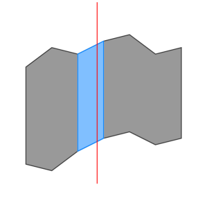
Figure 12. In this picture the grey region is $C_{{\boldsymbol{e}},\varepsilon}$, the red line is $\{x=x_{i}\}$ and the blue region is $V_{x_{i},\varepsilon}$.

Similarly, for each $\varepsilon>0$ and each integer $1<i\leq n$ define the set

$$R_{x_{i},\varepsilon}=:C_{{\boldsymbol{e}},\varepsilon}\cap\{x_{k_{(i-1),\varepsilon},\varepsilon}\leq x\leq x_{j_{i,\varepsilon},\varepsilon}\}$$

where $j_{i,\varepsilon}$ and $k_{i,\varepsilon}$ are defined as before. Then the set $R_{x_{i},\varepsilon}$ is the part of $C_{{\boldsymbol{e}},\varepsilon}$ which lies between $V_{x_{i-1},\varepsilon}$ and $V_{x_{i},\varepsilon}$.

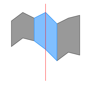
Figure 13. The region $V_{x_{i},\varepsilon}$ may be a hexagon if the line $\{x=x_{i}\}$ occurs at a vertex of $C_{{\boldsymbol{e}},\varepsilon}$.

Dividing $C_{{\boldsymbol{e}},0}$ among the sets $R_{x_{i},0}$ and recalling that these sets overlap on $V_{x_{i},0}$ we see that

$$N^{C_{{\boldsymbol{e}},0}}=\sum_{i=1}^{n}N^{R_{x_{i},0}}-\sum_{i=1}^{n-1}N^{V_{x_{i},0}}$$ (5.7)

Dividing $C_{{\boldsymbol{e}},\varepsilon}$ among the sets $R_{x_{i},\varepsilon}$ and the sets $V_{x_{i},\varepsilon}$ we see that

$$N^{C_{{\boldsymbol{e}},\varepsilon}}=\sum_{i=1}^{n}N^{R_{x_{i},\varepsilon}}+\sum_{i=1}^{n-1}N^{V_{x_{i},\varepsilon}}-\sum_{i=1}^{n-1}N^{R_{x_{i},\varepsilon}\cap V_{x_{i},\varepsilon}}-\sum_{i=1}^{n-1}N^{V_{x_{i},\varepsilon}\cap R_{x_{i+1},\varepsilon}}$$ (5.8)

Although (5.8) looks considerably more complicated than (5.7) note that (5.8) will converge to (5.7) if the following three equations are true:

$$\lim_{\varepsilon\searrow 0}N^{R_{x_{i},\varepsilon}}=N^{R_{x_{i},0}}$$ (5.9a)

$$\lim_{\varepsilon\searrow 0}N^{V_{x_{i},\varepsilon}}=N^{V_{x_{i},0}}$$ (5.9b)

$$\lim_{\varepsilon\searrow 0}N^{R_{x_{i},\varepsilon}\cap V_{x_{i},\varepsilon}}=\lim_{\varepsilon\searrow 0}N^{V_{x_{i},\varepsilon}\cap R_{x_{i+1},\varepsilon}}=N^{V_{x_{i},0}}$$ (5.9c)

We will prove these equations in reverse order.

Proof of (5.9c). We start by proving

$$\lim_{\varepsilon\searrow 0}N^{R_{x_{i},\varepsilon}\cap V_{x_{i},\varepsilon}}=N^{V_{x_{i},0}}$$

Note that the intersection of $R_{x_{i},\varepsilon}$ and $V_{x_{i},\varepsilon}$ is a line segment. The set $V_{x_{i},0}$ is also a line segment, so to prove the convergence of normal cycles we can use Lemma 5.6. For sufficiently small $\varepsilon$ we can assume that no vertex of $S$ occurs in between $R_{x_{i},\varepsilon}\cap V_{x_{i},\varepsilon}$ and $V_{x_{i},0}$. Then the top vertex of $R_{x_{i},\varepsilon}\cap V_{x_{i},\varepsilon}$ will differ in $x$-coordinate from the top vertex of $V_{x_{i},0}$ by at most the width of a line segment in $C_{{\boldsymbol{e}},\varepsilon}$ and differ in $y$-coordinate by a number proportional to the width of the line segment. This means that the distance from the top vertex of $R_{x_{i},\varepsilon}\cap V_{x_{i},\varepsilon}$ to the top vertex of $V_{x_{i},0}$ is $O(\varepsilon\sigma(\varepsilon))$. The same is true of the bottom vertices. Therefore Lemma 5.6 implies that

$$\lim_{\varepsilon\searrow 0}N^{R_{x_{i},\varepsilon}\cap V_{x_{i},\varepsilon}}=N^{V_{x_{i},0}}.$$

The above reasoning can be repeated to show that

$$\lim_{\varepsilon\searrow 0}N^{V_{x_{i},\varepsilon}\cap R_{x_{i+1},\varepsilon}}=N^{V_{x_{i},0}}$$

which completes the proof of (5.9c).

Proof of (5.9b). We once again make use of the inclusion-exclusion principle satisfied by the Normal Cycle. Divide the set $V_{x_{i},\varepsilon}$ into the following two sets:

$$V_{x_{i},\varepsilon}^{0}:=((\infty,x_{i}]\times\mathbb{R})\cap V_{x_{i},\varepsilon},\;\;V_{x_{i},\varepsilon}^{1}:=([x_{i},\infty)\times\mathbb{R})\cap V_{x_{i},\varepsilon}.$$

Then we have

$$N^{V_{x_{i},\varepsilon}}=N^{V_{x_{i},\varepsilon}^{0}}+N^{V_{x_{i},\varepsilon}^{1}}-N^{V_{x_{i},\varepsilon}^{0}\cap V_{x_{i},\varepsilon}^{1}}$$

so that (5.9b) will hold if $N^{V_{x_{i},\varepsilon}^{0}}$, $N^{V_{x_{i},\varepsilon}^{1}}$ and $N^{V_{x_{i},\varepsilon}^{0}\cap V_{x_{i},\varepsilon}^{1}}$ all converge to $N^{V_{x_{i},0}}$.

Note that the set $V_{x_{i},\varepsilon}^{0}\cap V_{x_{i},\varepsilon}^{1}$ is a line segment. If the top and bottom vertex of $V_{x_{i},\varepsilon}^{0}\cap V_{x_{i},\varepsilon}^{1}$ are sample points of the approximation, then Proposition 2.3 implies that the Hausdorff distance from $V_{x_{i},\varepsilon}^{0}\cap V_{x_{i},\varepsilon}^{1}$ to $V_{x_{i},0}$ is $O(\alpha\varepsilon)$. If the top and bottom vertices of the line segment are not sample points of the approximation, note that they differ in width from a sample point by at most $\varepsilon\sigma(\varepsilon)$. Therefore in all cases the Hausdorff distance from $V_{x_{i},\varepsilon}^{0}\cap V_{x_{i},\varepsilon}^{1}$ to $V_{x_{i},0}$ is $O(\alpha\varepsilon+\alpha\varepsilon\sigma(\varepsilon))$. This vanishes as $\varepsilon\to 0$, so that Lemma 5.6 implies that

$$\lim_{\varepsilon\searrow 0}N^{V_{x_{i},\varepsilon}^{0}\cap V_{x_{i},\varepsilon}^{1}}=N^{V_{x_{i},0}}$$

Note that each set $V_{x_{i},\varepsilon}^{0}$ and $V_{x_{i},\varepsilon}^{1}$ must be a convex quadrilateral. The width of their union $V_{x_{i},\varepsilon}$ is $O(\varepsilon\sigma(\varepsilon))$ by construction. This implies that the widths of each of $V_{x_{i},\varepsilon}^{0}$ and $V_{x_{i},\varepsilon}^{1}$ vanish as $\varepsilon\to 0$. Therefore each set converges to $V_{x_{i},\varepsilon}^{0}\cap V_{x_{i},\varepsilon}^{1}$ in Hausdorff distance as $\varepsilon\to 0$. This implies

$$\lim_{\varepsilon\searrow 0}N^{V_{x_{i},\varepsilon}^{0}}=\lim_{\varepsilon\searrow 0}N^{V_{x_{i},\varepsilon}^{1}}=N^{V_{x_{i},0}}$$

completing the proof of (5.9b).

Proof of (5.9a). The major difficulty in this case is that the regions $R_{x_{i},\varepsilon}$ need not be convex polygons so we cannot apply Lemma 5.6. Thus we must return to proving the three conditions of Theorem 5.5 directly.

Note that each $R_{x_{i},\varepsilon}$ can be considered the PL approximation with spread $\sigma(\varepsilon)$ of the region $R_{x_{i},0}$. The region $R_{x_{i},0}$ is simply an elementary set which lies between two line segments. Theorem 2.11 implies that the distance of the boundary of $R_{x_{i},\varepsilon}$ to the boundary of $R_{x_{i},0}$ is $O(\varepsilon+\varepsilon\sigma(\varepsilon)+(\varepsilon\sigma(\varepsilon))^{2})$. Therefore the sets $R_{x_{i},\varepsilon}$ must all be contained in some compact subset of $\mathbb{R}^{2}$.

Since $R_{x_{i},\varepsilon}$ is the PL approximation of an elementary set with spread $\sigma(\varepsilon)$, Corollary 3.7 implies that the total curvature of its boundary converges to the total curvature of the boundary of $R_{x_{i},0}$. The computations of [20, Chap. 23] show that the mass of a normal cycle of a polygon is equal to the perimeter of the polygon plus the total curvature of its boundary. Therefore the mass of $N^{R_{x_{i},\varepsilon}}$ cannot increase to infinity.

The final condition to prove from Theorem 5.5 is that the Euler characteristic of intersection of $R_{x_{i},\varepsilon}$ with any generic half-plane converges to the Euler characteristic of the intersection of $R_{x_{i},0}$ with the same half-plane. To prove this we will need a technical lemma whose proof we will defer until later.

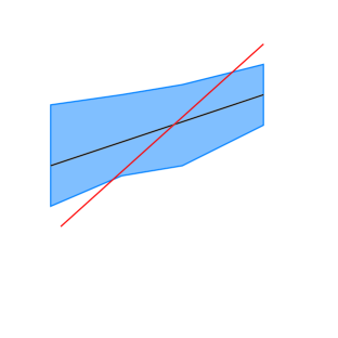
Figure 14. The situation of Lemma 5.7. The red line only intersects the boundary of the blue approximation twice.

Lemma 5.7.

Let $S$ be a single non-vertical line segment and for each $\varepsilon>0$ let $\Xi_{\varepsilon}$ an upper or lower sample of $S$ with spread $\sigma(\varepsilon)$ and for every $\varepsilon$ let $f_{\varepsilon}$ indicate the PL-approximation of $S$ determined by $\Xi_{\varepsilon}$.

Let $\xi\in\operatorname{Hom}(\mathbb{R}_{2},\mathbb{R})$ and suppose that the line $\{\xi=c\}$ is not parallel to $S$ and intersects $S$. Then there exists a $\varepsilon^{*}>0$ depending only on $S$ and $\xi$ such that for $0<\varepsilon<\varepsilon_{0}$, the line $\{\xi=c\}$ intersects the graph of $f_{\varepsilon}$ exactly once. $\hbox to0.0pt{$\sqcap$\hss}\sqcup$

Given this lemma, fix a $c\in\mathbb{R}$ and a $\xi\in\operatorname{Hom}(\mathbb{R}^{2},\mathbb{R})$ such that the line $\{\xi=c\}$ is not parallel to a line segment of $R_{x_{i},0}$. We distinguish two cases.

A. The line $\{\xi=c\}$ does not intersect $R_{x_{i},0}$. Theorem 2.11 implies that for all sufficiently small $\varepsilon$, the line $\{\xi=c\}$ will not intersect $R_{x_{i},\varepsilon}$. Since $R_{x_{i},\varepsilon}$ converges to $R_{x_{i},0}$ in Hausdorff measure, the half-plane will contain $R_{x_{i},\varepsilon}$ for small $\varepsilon$ if and only if it contains $R_{x_{i},0}$. The sets $R_{x_{i},0}$ and $R_{x_{i},\varepsilon}$ both must be contractible since they are regions which lie between the graphs of two piecewise linear functions which do not intersect. Therefore in this case

$$\lim_{\varepsilon\searrow 0}\chi(\{\xi\geq c\}\cap R_{x_{i},\varepsilon})=\chi(\{\xi\geq c\}\cap R_{x_{i},0}).$$

B. The line $\{\xi=c\}$ does intersect the set $R_{x_{i},0}$. Since $R_{x_{i},0}$ is convex, we clearly have

$$\chi(\{\xi\geq c\}\cap R_{x_{i},0})=1.$$

Let $\varepsilon\in(0,\varepsilon^{*}(R_{x_{i},0}))$, where $\varepsilon^{*}(R_{x_{i},0})$ is the constant guaranteed by Lemma 5.7. Then the desired convergence in Euler characteristic is an immediate consequence of the following lemma.

Lemma 5.8.

(a) For any $d\geq c$ the intersection between the line $\{\xi=d\}$ and $R_{x_{i},\varepsilon}$ is either empty or a closed segment (possibly degenerate).

(b) $\chi\bigl{(}\,\{\xi\geq c\}\cap R_{x_{i},\varepsilon}\,\bigr{)}=1.$

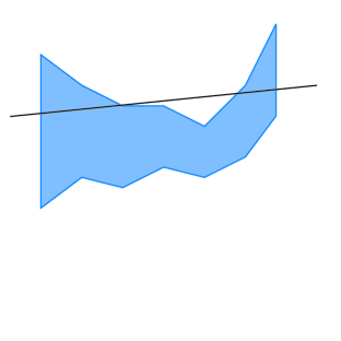
Figure 15. For a line to intersect $R_{x_{i},\varepsilon}$ in a non-connected fashion it must intersect either the upper or the lower boundary multiple times.

Proof.

(a) Assume that the line $\{\xi=d\}$ is the graph of the linear function $\ell(x)=mx+b$. The boundary of $R_{x_{i},\varepsilon}$ has four component: a top, a bottom and two vertical side components. The top and boundary components are graphs of $PL$ functions $T_{\varepsilon}(x)$ and respectively $B_{\varepsilon}(x)$ (see Figure 15). Lemma 5.7 implies that each line $\{\xi=d\}$ intersects each of these components at most once so the intersection between the line $\{\xi=d\}$ and the boundary of $R_{x_{i},\varepsilon}$ consists of at most four points.

We consider the set $\{\xi=d\}\cap R_{x_{i},\varepsilon}$ which is the union of some number of line segments. Let $p_{1},p_{2},\dots p_{n}$, $n\leq 4$, be the endpoints of these line segments arranged increasingly according to their $x$-coordinates. We claim that $n\leq 2$ so that the intersection between $\{\xi=d\}$ and $R_{x_{i},\varepsilon}$ is a (possibly degenerate) line segment. To prove this we argue by contradiction.

Suppose that the intersection consists of at least three points $p_{1},p_{2},p_{3}$. Let $(t_{j},u_{j})$ be the coordinates of $p_{j}$, $1\leq j\leq 3$, so that $t_{1}<t_{2}<t_{3}$. Think of the line $\{\xi=d\}$ as the trajectory of a particle moving in the plane with constant velocity

$$x=t,\;\;y=\ell(t)=mt+b.$$

The particle first enters $R_{x_{i},\varepsilon}$ at the moment $t=t_{1}$ and exits at the moment $t=t_{2}$. Note that the corresponding exit point $p_{2}$ cannot be on either one of the vertical components of the boundary of $R_{x_{i},\varepsilon}$ so it must be either on the top part or on the bottom of the boundary. Assume that $p_{2}$ is on the top part of the boundary. (The case when $p_{2}$ is on the bottom is dealt with in a similar fashion.)

Lemma 5.7 implies that the particle will never intersect the top part of the boundary ever again so that

$$\ell(t)>T_{\varepsilon}(t)\geq B_{\varepsilon}(t),\;\;\forall t>t_{2}.$$

This implies that at the moment $t_{3}$ when the particle enters $R_{x_{i},\varepsilon}$ again, it must do so through one of the vertical portions of the boundary of $R_{x_{i},\varepsilon}$. On the other hand at that moment we have

$$u_{3}=\ell(t_{3})>T_{\varepsilon}(t_{3})\geq B_{\varepsilon}(t_{3}).$$

so the point $p_{3}$ cannot lie on the vertical segment

$$\bigl{\{}(t_{3},y);B_{\varepsilon}(t_{3})\leq y\leq T_{\varepsilon}(t_{3})\,\bigr{\}}$$

which the rightmost part of the boundary of $R_{x_{i},\varepsilon}$.

(b) Set for simplicity

$$R_{x_{i},\varepsilon}^{\xi\geq c}:=\bigl{\{}\xi\geq c\}\cap R_{x_{i},\varepsilon}.$$

Observe that the set $I_{c}:=\xi\bigl{(}R_{x_{i},\varepsilon}^{\xi\geq c}\,\bigr{)}\subset\mathbb{R}$ is connected because $\xi(R_{x_{i},\varepsilon})$ is a closed interval and

$$I_{c}=\xi(R_{x_{i},\varepsilon})\cap[c,\infty).$$

The map $\xi$ defines a continuous surjection $\xi:R_{x_{i},\varepsilon}^{\xi\geq c}\rightarrow I_{c}$ with contractible fibers. The Vietoris-Biegle theorem, [23, Thm.15, Chap.6, Sec.9] implies that $R_{x_{i},\varepsilon}^{\xi\geq c}$ has the same coh $\hbox to0.0pt{$\sqcap$\hss}\sqcup$

To complete the proof of (5.9a) (and consequently also prove (5.6b), Lemma 5.4 and the overall Theorem5.1) we need only prove Lemma 5.7

Proof of Lemma 5.7. Let $\alpha$ be the slope of $S$. Suppose that $\xi(x_{1},x_{2})=\xi_{1}x_{1}+\xi_{2}x_{2}$. Then

$$\xi_{1}+\xi_{2}\alpha\neq 0$$

since $S$ is not parallel to $\{\xi=c\}$. The function $f_{\varepsilon}$ is differentiable every where except at a finite number of points. Theorem 2.11 implies that there exists an $\varepsilon_{0}>0$ such that for $0<\varepsilon<\varepsilon_{0}$,

$$\xi_{1}+f_{\varepsilon}^{\prime}(x)\xi_{2}$$

is either strictly positive or strictly negative for all $x$ in the domain of $f_{\varepsilon}$ since $f^{\prime}_{\varepsilon}(x)$ must be close to $\alpha$ and $\xi_{1}+\xi_{2}\alpha\neq 0$. We set $\xi|_{f_{\varepsilon}}(x)=\xi_{1}x+\xi_{2}f(x)$. The notation indicates that $\xi|_{f_{\varepsilon}}$ is the restriction of $\xi$ to the graph of $f_{\varepsilon}$. Note that $\xi|_{f_{\varepsilon}}$ is Lipschitz and

$$\frac{d\xi|_{f_{\varepsilon}}}{dx}(x)=\xi_{1}+\xi_{2}f_{\varepsilon}^{\prime}(x),$$

for all but finitely many $x$.

Now suppose that $\{\xi=c\}$ intersects the graph of $f_{\varepsilon}$ at points $(x_{0},y_{0})$ and $(x_{1},y_{1})$. Then note $\xi|_{f_{\varepsilon}}$ is equal to $c$ for $x_{0}$ and $x_{1}$. Thus we have, [24, Prop. 11.12]

$$0=\xi|_{f_{\varepsilon}}(x_{1})-\xi_{\varepsilon}(x_{0})=\int_{x_{0}}^{x_{1}}\frac{d\xi|_{f_{\varepsilon}}}{dx}dx=\int_{x_{0}}^{x_{1}}\bigl{(}\xi_{1}+\xi_{2}f_{\varepsilon}^{\prime}(x)\,\bigr{)}dx.$$

But $\xi_{1}+\xi_{2}f_{\varepsilon}^{\prime}(x)$ is either strictly positive or strictly negative. Therefore the integral

$$\int_{x_{0}}^{x_{1}}\frac{d\xi|_{f_{\varepsilon}}}{dx}dx$$

cannot be 0, contradicting our assumption that $\{\xi=c\}$ intersects the graph of $f_{\varepsilon}$ at two points. This completes the proof of Lemma 5.7 $\hbox to0.0pt{$\sqcap$\hss}\sqcup$

Appendix A The Farey Series and Holes in Pixelations

An unintuitive feature of pixelations is that they do not preserve homotopy type, even for small values of $\varepsilon$. The Figure 10 in Section 4 gives an example of a contractible set whose $\varepsilon$-pixelations always contain a cycle. In this appendix we wish to expand on the nature of these “holes” as well as show that an arbitrary number of such holes can appear.

We start by defining a convenient class of sets.

Definition A.1.

The angle with slopes $(\alpha,\beta)$, where $\beta>\alpha$ is the set

$$A(\beta,\alpha):=\bigl{\{}\,(x,y)\in\mathbb{R}^{2}:\;\;x\geq 0,\;\;(y-\alpha x)(y-\beta x)=0\,\bigr{\}}.$$

Angles are convenient to work with in the context of pixelations since they have nice self similarity properties. Note that

$$P_{\varepsilon}(A(\beta,\alpha))=\varepsilon P_{1}(A(\beta,\alpha))$$

where the last equality holds because $A(\beta,\alpha)$ does not change under rescalings centered at the origin. This means that different $\varepsilon$-pixelations are simply retractions or expansions of any other $\varepsilon$-pixelation, and are thus topologically equivalent. Therefore if a cycle appears in any $\varepsilon$-pixelation of an angle, it will appear in every $\varepsilon$-pixelation of an angle. We refer to these false cycles in the $\varepsilon$-pixelations as holes.

Figure 16 is an example of a pixelation of an angle that has a hole, and in particular, the pixelation is not contractible, while an angle plainly is.

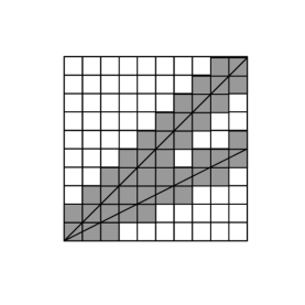
Figure 16. The pixelation of the angle $A\left(1,\frac{1}{2}\right)$ contains 1 hole in the 7th column from the $y$-axis.

When varying the slopes of the angle $A(\beta,\alpha)$ several things become apparent. First, for a hole to appear either both slopes must be positive or both slopes must be negative. Second, the two lines must have fairly close slopes for holes to appear. Finally, more holes will tend to appear when one of the slopes is close to $1$.

It is beyond the scope of this paper to classify the behavior of holes for general angles. However, an easier situation occurs when the two slopes of the angle are adjacent members of a Farey series.

The $n$-th Farey series $F_{n}$ is the increasing finite sequence consisting of the rational numbers between $0$ and $1$ which have denominator of $n$ or less when written in lowest terms. For example,

$$F_{4}={\frac{0}{1},\frac{1}{4},\frac{1}{3},\frac{1}{2},\frac{2}{3},\frac{3}{4},\frac{1}{1}}$$

An important property of the Farey sequences is that if $\frac{a}{b}$ and $\frac{c}{d}$ are consecutive terms in a Farey series, then $bc-ad=1$, [12, Chap.III]. Using this property, we can prove the following fact.

Proposition A.2.

Suppose $\frac{a}{b}$ and $\frac{c}{d}$ are consecutive terms in a Farey series. Denote by $g(a,b;c,d)$ the number of holes of the $\varepsilon$-pixelation

$$P_{\varepsilon}\left(A\left(\frac{c}{d},\frac{a}{b}\right)\right),$$

and by $X_{a,b,c,d}$ the set of lattice points $(p,q)\in\mathbb{Z}^{2}$ such that

$$0<p\leq d,$$ (A.1)

$$a<q\leq\min(2a,b),$$

$$bd+bc+b+d\leq 1+pb+qd<2bd+bc+b+d.$$

Then

$$g(a,b;c,d):=ad-\#X_{a,b,c,d}$$

Proof.

As noted in the earlier discussion, any $\varepsilon$-pixelation of the angle is topologically equivalent to $P_{1}\left(A\left(\frac{c}{d},\frac{a}{b}\right)\right)$. Therefore we need only to consider the case $\varepsilon=1$. We set

$$m_{1}:=\frac{c}{d},\;\;m_{0}:=\frac{a}{b}.$$

For $j=0,1$ we denote by $\ell_{j}$ the half-line

$$y=m_{j}x,\;\;x\geq 0.$$

For each $i\in\mathbb{Z}_{>0}$ we define (using the notations in Definition 2.1)

$$U_{i}:=B_{1}\left(\ell_{1},\frac{2i-1}{2}\right)=\begin{cases}\left\lfloor m_{1}(i-1)\right\rfloor,&m_{1}(i-1)\not\in\mathbb{Z}\\ &\\ m_{1}(i-1)-1,&m_{1}(i-1)\in\mathbb{Z}\end{cases},$$ (A.2)

$$L_{i}:=T_{1}\left(\ell_{0},\frac{2i-1}{2}\right)=\begin{cases}\left\lceil m_{0}i\right\rceil,&m_{0}i\not\in\mathbb{Z}\\ &\\ m_{0}i+1,&m_{0}i\in\mathbb{Z}\end{cases}.$$ (A.3)

In other words, $U_{i}$ indicates the lowest $y$-value of the $1$-pixelation of the half-line $\ell_{1}$ within the $i$-th column $[i-1,i]\times\mathbb{R}$, and $L_{i}$ indicates the highest $y$-value of the $1$-pixelation of the half-line $\ell_{0}$ in the same column. Set $D_{i}:=U_{i}-L_{i}$ and observe that (A.2) and (A.3) imply

$$D_{i}<(m_{1}-m_{0})i=\frac{i}{bd}.$$ (A.4)

Note also that

$$D_{1}=-2,\;\;D_{2}\in\{-1,-2\}.$$ (A.5)

More generally, (A.4) implies that

$$D_{i}\leq 0,\;\;\forall i=1,\dotsc,bd.$$ (A.6)

The quantities $U_{i}$ and $L_{i}$ are useful because they allow us to easily state when there is a gap in a column or on the edge of a column. The $i$-th columns of the pixelations of the upper and lower half-lines overlap if and only if

$$U_{i}\leq L_{i}$$

and the two pixelations overlap on the right side of the $i$-th column if and only if

$$U_{i}\leq L_{i+1}$$

A hole is a gap which is closed on both sides. In particular, it is closed on the right side. This means in each hole there is a column where the pixelations of $\ell_{0}$ and $\ell_{1}$ do not overlap on the interior of the column, but do overlap on the right side of the column. In terms of $U_{i}$ and $L_{i}$ this is equivalent to the condition

$$L_{i}<U_{i}\leq L_{i+1}$$ (A.7)

Note that this condition only occurs when $L_{i+1}>L_{i}$. Since $\frac{a}{b}\leq 1$ we have

$$L_{i+1}\leq L_{i}+1$$

This means that the condition $L_{i+1}>L_{i}$ is equivalent to the condition $L_{i+1}=L_{i}+1$.

Suppose that $U_{i}-L_{i}=2$. Then it is impossible that $U_{i}\leq L_{i+1}$ since that would imply that the lower line increased by at least the length of a pixel in the amount of time that the upper line increased by less than the length of a pixel. Therefore for (A.7) to occur, it must be true that $U_{i}-L_{i}=1$. Combining this fact with the above discussion about $L_{i}$ and $L_{i+1}$, we find that (A.7) is equivalent to the condition

$$U_{i}-L_{i}=1\text{ and }L_{i+1}=L_{i}+1.$$ (A.8)

Note that $L_{i}$ increases by $c$ every $d$ columns since $\ell_{1}$ has slope $\frac{c}{d}$. Hence

$$U_{i+d}=U_{i}+c,$$

and similarly

$$L_{i+b}=L_{i}+a.$$

Therefore

$$U_{i+bd}-L_{i+bd}=U_{i}+bc-(L_{i}+ad)=U_{i}-L_{i}+(bc-ad)=U_{i}-L_{i}+1,$$

so that

$$D_{i+bd}=D_{i}+1.$$ (A.9)

We set

$$k_{1}:=\min\{k\in\mathbb{Z}_{>0};\;\;D_{k}=1\,\bigr{\}}.$$

We know that $k_{1}$ exists since (A.9) and (A.5) imply that $D_{i}$ takes on every integer value greater than or equal to $1$. Note that (A.4) implies that, if $k_{1}$ exists, then $k_{1}>bd$. To finish the proof we will need a variety of facts about $k_{1}$.

Lemma A.3.

(a) $k_{1}:=(a+1)d+b+1+bd=bd+bc+b+d$.

(b) For any $i\in[k_{1},k_{1}+bd)\cap\mathbb{Z}$ we have

$$0\leq D_{i}<2$$ (A.10)

(c) For any $i\geq k_{1}+bd$ we have $D_{i}>0$.

Proof.

(a) The inequality (A.4) implies that $k_{1}>bd$ so that

$$k_{0}:=k_{1}-bd>0$$

and

$$D_{k_{0}}=0.$$

Moreover, the minimality of $k_{1}$ coupled with (A.9) implies that

$$k_{0}=\min\{i>0;\;\;D_{i}=0\,\}.$$

If $D_{i}=0$ then there exists a positive integer $\ell$ such that

$$\ell-1\leq m_{0}(i-1)<m_{0}i<\ell.$$ (A.11a)

$$\ell<m_{1}(i-1)\leq\ell+1$$ (A.11b)

When these conditions are satisfied we have $U_{i}=L_{i}=\ell$. The lattice point $(i-1,\ell)$ is in the interior of the angle $A(m_{1},m_{0})$ spanned by the vectors

$$\vec{u}_{1}=(b,a),\;\;\vec{u}_{2}=(d,c).$$

Since $bc-ad=1$ we deduce that the vectors $\vec{u}_{1},\vec{u_{2}}$ form an integral basis of the lattice $\mathbb{Z}^{2}$. We deduce that there exist two positive integers $p,q$ such that

$$(i-1,\ell)=p\vec{u}_{1}+q\vec{u_{2}},\;\;\mbox{i.e.,}\;\;i-1=pb+qd,\;\;\ell=pa+qc.$$

Observe that

$$m_{0}(i-1)=\frac{a}{b}(pb+qd)=ap+q\frac{ad}{b}=ap+q\frac{bc-1}{b}=ap+qc-\frac{q}{b}=\ell-\frac{q}{b}.$$

Hence (A.11a) is satisfied if and only if

$$a<q\leq b.$$ (A.12)

On the other hand,

$$m_{1}(i-1)=\frac{c}{d}(pb+qd)=p\frac{bc}{d}+qc=p\frac{ad+1}{d}+qc=pa+qc+\frac{p}{d}=\ell+\frac{p}{d}.$$

Hence (A.11b) is satisfied when

$$0<p\leq d.$$ (A.13)

From the equality

$$i=1+pb+qd$$

we deduce that

$$\min\{i>0;D_{i}=0\}=\min\{1+pb+qd;\;\;0<p\leq d,\;\;a<q\leq b\,\}=1+b+(a+1)d.$$

This proves (a).

(b) To prove the upper estimate in (A.10) we use (A.4). For $i<k_{1}+bd$ we have

$$D_{i}<1+\frac{k_{1}}{bd}=1+\frac{(a+1)d+b+1}{bd}=1+\frac{a+1}{b}+\frac{b+1}{bd}<3.$$

Thus $D_{i}\leq 2$ for all $i\in[k_{1},k_{1}+bd)\cap\mathbb{Z}$. If $D_{i}=2$ for some $i$ in this range then $D_{i-bd}=1$, contradicting the minimality of $k_{1}$.

To prove the lower estimate part of (A.10) we recall that

$$k_{0}=k_{1}-bd=\min\{\,k>0;\;\;D_{k}=0\,\}.$$

Let us observe that

$$D_{i}\geq-1,\;\;\forall i\geq k_{0}.$$

Indeed the inequality $D_{i}<-1$ takes place only if $m_{0}i\geq\ell\in\mathbb{Z}$ and $m_{1}(i-1)\leq\ell$. This implies

$$m_{1}(i-1)\leq m_{0}i\Longleftrightarrow\frac{i}{bd}\leq\frac{c}{d}\Longleftrightarrow i\leq bc=ad+1<k_{0}.$$

Hence, for any $i\geq k_{0}+bd$ we have $D_{i}\geq 0$ proving part (b). Part (c) follows from (b) and (A.9). $\hbox to0.0pt{$\sqcap$\hss}\sqcup$

This lemma narrows down the possible locations of holes. In particular, property (c) implies that holes can only occur in columns in the interval $[k_{1},k_{1}+bd)$. Recall that for a hole to appear, we need $L_{i+1}=L_{i}+1$ and $D_{i}=1$. In most cases when $L_{i}$ increases in this interval $D_{i}$ will also be equal to $1$. However, if $U_{i+1}=U_{i}+1$, $L_{i+1}=L_{i}+1$ and $D_{i}=0$, then no hole appears. We want to count these instances where an increase in $L_{i}$ does not indicate the presence of a hole through the use of the set $X_{a,b,c,d}$. We do this through a series of lemmas.

Define a map

$$\Phi:X_{a,b,c,d}\rightarrow\mathbb{Z},\;\;(p,q)\mapsto 1+pb+qd.$$

Lemma A.4.

The map $\Phi$ is injective.

Proof.

Indeed if $\Phi(p,q)=\Phi(p^{\prime},q^{\prime})$ then $(p-p^{\prime})b=(q^{\prime}-q)d$. Since $b$ and $d$ are coprime we deduce that $(p-p^{\prime})$ must be a multiple of $d$. Since $0<p,p^{\prime}\leq d$ this happens if and only if $p=p^{\prime}$. It automatically follows that $q=q^{\prime}$. $\hbox to0.0pt{$\sqcap$\hss}\sqcup$

We denote by $I_{a,b,c,d}$ the range of $\Phi$. From the definition of $X_{a,b,c,d}$ we deduce that

$$I_{a,b,c,d}\subset[k_{1},k_{1}+bd).$$

Lemma A.5.

The following statements are equivalent.

(a) $i\in[k_{1},k_{1}+bd)\cap\mathbb{Z}$, $U_{i}=L_{i}$ and $L_{i+1}=L_{i}$.

(b) $i\in I_{a,b,c,d}$

Proof.

Let $i\in[k_{1},k_{1}+bd)\cap\mathbb{Z}$ such that $L_{i+1}=L_{i}+1$ and $D_{i}=0$. Using the notation and the terminology employed in the proof of Lemma A.10(a) we deduce that the condition $D_{i}=0$ holds if and only if that there exist positive an integer $\ell$ such that (A.11a) and (A.11b) hold. Moreover

$$i=1+pb+qd,$$

where $q$ and $p$ are constrained by (A.12) and (A.13). Once the condition $D_{i}=0$ is satisfied the condition $L_{i+1}=L_{i}+1=\ell+1$ is equivalent to

$$\ell\leq m_{0}(i+1)<\ell+1.$$

$$m_{0}(i+1)=m_{0}(i-1)+2m_{0}=\ell+\frac{2a-q}{b}\geq\ell.$$

Hence $a<q\leq\min(b,2a)$, $0<p\leq d$, and $i=\Phi(p,q)$, $(p,q)\in X_{a,b,c,d}$, i.e., $i\in I_{a,b,c,d}$. $\hbox to0.0pt{$\sqcap$\hss}\sqcup$

Lemma A.10(c) shows that the conditions of (A.8) cannot be met in the $(k+bd)$-th column and beyond. Therefore, the right edge of any hole must occur between the $k$-th column and the $(k+bd)$-th column. Therefore the pixelation of the angle contains a hole for each time that $U_{i}-L_{i}=1$ and $L_{i}$ increases between the $k$-th and $(k+bd)$-th column (including $k$ but not $(k+bd)$.) and This is a total of $bd$ columns, and $L_{i}$ increases by $a$ every $b$ columns. Hence $L_{i}$ will increase $ad$ times in this range. On the other hand if $i\in I_{a,b,c,d}$ the $L_{i}$ increases yet $U_{i}=L_{i}$. Therefore $P_{\varepsilon}\left(A\left(\frac{c}{d},\frac{a}{b}\right)\right)$ contains $ad-\#I_{a,b,c,d}$ holes. The conclusion of the proposition follows from the injectivity of $\Phi$. $\hbox to0.0pt{$\sqcap$\hss}\sqcup$

Remark A.6.

The proof of Proposition A.2 gives us a simple algorithm for computing $g(a,b;c,d)$ that is easily implementable numerically. More precisely we have

$$g(a,b;c,d)=\sum_{i=k_{1}}^{k_{1}+bd-1}(U_{i}-L_{i})(L_{i+1}-L_{i}). \hbox to0.0pt{$\sqcap$\hss}\sqcup$$

Corollary A.7.

$$g(n,2n+1;1,2)=2n. \hbox to0.0pt{$\sqcap$\hss}\sqcup$$

Proof.

In this case the set $X_{n,2n+1,1,2}$ is empty and the above equality follows immediately from Proposition A.2. $\hbox to0.0pt{$\sqcap$\hss}\sqcup$

The above corollary shows that the pixelation of even a very simple set can have a complicated homotopy type.

Example A.8.

Let us consider the following situation

$$\frac{c}{d}=\frac{1}{2},\;\;\frac{a}{b}=\frac{2}{5}.$$

Then

$$U_{i+2}=U_{i}+1,\;\;L_{j+5}=L_{j}+2,\;\;D_{i+10}=D_{i}+1.$$

Using (A.2), (A.3) and the above equalities we get

$$i$$

Using this table and (A.9) we deduce that $k=22$. Next, using the above table and the equalities

$$U_{i+20}=U_{i}+10,\;\;L_{i+20}=L_{i}+8$$

we obtain the following table

$$i$$

In this case there are five holes. Two holes are immediately apparent, since in the $23$rd and $25$th column a distance of $1$ is followed by a distance of $0$. However note that in the $26$th column we have $D_{26}$ of $1$ and then $U_{26}=L_{27}$. This indicates that a hole is formed merely because the pixelations of the upper and lower lines touch at a corner (compare to the case of Figure 16.) Similar holes exist in the $27$th column and the $29$th column. No holes exist past this point, since Lemma A.10 implies that past this point $D_{i}>0$. $\hbox to0.0pt{$\sqcap$\hss}\sqcup$

Appendix B Subanalytic Currents

In this appendix we gather without proofs a few facts about the subanalytic currents introduced by R. Hardt in [10, 11]. Our terminology concerning currents closely follows that of Federer [5] (see also the more accessible [16, 20]). However, we changed some notations to better resemble notations used in algebraic topology. First we need to define the subanalytic sets.

An $\mathbb{R}$-structure is a collection $\mathcal{S}=\bigl{\{}\,\mathcal{S}^{n}\,\bigr{\}}_{n\geq 1}$, $\mathcal{S}^{n}\subset\mathcal{P}(\mathbb{R}^{n})$, with the following properties.

${\bf E}_{1}.$:

$\mathcal{S}^{n}$ contains all the real algebraic subvarieties of $\mathbb{R}^{n}$, i.e., the zero sets of finite collections of polynomial in $n$ real variables.

${\bf E}_{2}.$:

For every linear map $L:\mathbb{R}^{n}\rightarrow\mathbb{R}$, the half-plane $\{\vec{x}\in\mathbb{R}^{n};\;\;L(x)\geq 0\}$ belongs to $\mathcal{S}^{n}$.

${\bf P}_{1}.$:

For every $n\geq 1$, the family $\mathcal{S}^{n}$ is closed under boolean operations, $\cup$, $\cap$ and complement.

${\bf P}_{2}.$:

If $A\in\mathcal{S}^{m}$, and $B\in\mathcal{S}^{n}$, then $A\times B\in\mathcal{S}^{m+n}$.

${\bf P}_{3}.$:

If $A\in\mathcal{S}^{m}$, and $T:\mathbb{R}^{m}\rightarrow\mathbb{R}^{n}$ is an affine map, then $T(A)\in\mathcal{S}^{n}$.

Example B.1 (Semialgebraic sets).

Denote by $\mathbb{R}_{alg}$ the collection of real semialgebraic sets. Thus, $A\in\mathbb{R}^{n}_{alg}$ if and only if $A$ is a finite union of sets, each of which is described by finitely many polynomial equalities and inequalities. The celebrated Tarski-Seidenberg theorem states that $\mathcal{S}_{alg}$ is a structure. $\hbox to0.0pt{$\sqcap$\hss}\sqcup$

Let $\mathcal{S}$ be an $\mathbb{R}$-structure. Then a set that belongs to one of the $\mathcal{S}^{n}$-s is called $\mathcal{S}$-definable. If $A,B$ are $\mathcal{S}$-definable, then a function $f:A\rightarrow B$ is called $\mathcal{S}$-definable if its graph $\Gamma_{f}:=\bigl{\{}\,(a,b)\in A\times B;\;\;b=f(a)\,\bigr{\}}$ is $\mathcal{S}$-definable.

Given a collection $\mathcal{A}=(\mathcal{A}_{n})_{n\geq 1}$, $\mathcal{A}_{n}\subset\mathcal{P}(\mathbb{R}^{n})$, we can form a new structure $\mathcal{S}(\mathcal{A})$, which is the smallest structure containing $\mathcal{S}$ and the sets in $\mathcal{A}_{n}$. We say that $\mathcal{S}(\mathcal{A})$ is obtained from $\mathcal{S}$ by adjoining the collection $\mathcal{A}$.

Definition B.2.

An $\mathbb{R}$-structure is called $o$-minimal (order minimal) or tame if it satisfies the property

T:

Any set $A\in\mathcal{S}^{1}$ is a finite union of open intervals $(a,b)$, $-\infty\leq a<b\leq\infty$, and singletons $\{r\}$. $\hbox to0.0pt{$\sqcap$\hss}\sqcup$

Example B.3.

(a) (Tarski-Seidenberg) The collection $\mathbb{R}_{alg}$ of real semialgebraic sets is a tame structure.

(b) (A. Gabrielov, R. Hardt, H. Hironaka, [8, 11, 13]) A restricted real analytic function is a function $f:\mathbb{R}^{n}\rightarrow\mathbb{R}$ with the property that there exists a real analytic function $\tilde{f}$ defined in an open neighborhood $U$ of the cube $C_{n}:=[-1,1]^{n}$ such that

$$f(x)=\begin{cases}\tilde{f}(x)&x\in C_{n}\\ 0&x\in\mathbb{R}^{n}\setminus C_{n}.\end{cases}$$

we denote by $\mathbb{R}_{an}$ the structure obtained from $\mathcal{S}_{alg}$ by adjoining the graphs of all the restricted real analytic functions. Then $\mathbb{R}_{an}$ is a tame structure, and the $\mathbb{R}_{an}$-definable sets are called (globally) subanalytic sets. $\hbox to0.0pt{$\sqcap$\hss}\sqcup$

The definable sets and function of a tame structure have rather remarkable tame behavior which prohibits many pathologies. It is perhaps instructive to give an example of function which is not definable in any tame structure. For example, the function $x\mapsto\sin x$ is not definable in a tame structure because the intersection of its graph with the horizontal axis is the countable set $\pi\mathbb{Z}$ which violates the tameness condition ${\bf T}$.

We list below some of the nice properties of the sets and function definable in a fixed tame structure $\mathcal{S}$. Their proofs can be found in [3, 25]. We will interchangeably refer to sets or functions definable in a given tame structure $\mathcal{S}$ as definable, constructible or tame.

➣ (Piecewise smoothness of tame functions.) Suppose $A$ is a definable set, $p$ is a positive integer, and $f:A\rightarrow\mathbb{R}$ is a definable function. Then $A$ can be partitioned into finitely many definable sets $S_{1},\dotsc,S_{k}$, such that each $S_{i}$ is a $C^{p}$-manifold, and each of the restrictions $f|_{S_{i}}$ is a $C^{p}$-function.

➣ (Triangulability.) For every compact definable set $A$, and any finite collection of definable subsets $\{S_{1},\dotsc,S_{k}\}$, there exists a compact simplicial complex $K$, and a definable homeomorphism $\Phi:|K|\rightarrow A$ such that all the sets $\Phi^{-1}(S_{i})$ are unions of relative interiors of faces of $K$.

➣ (Dimension.) The dimension of a definable set $A\subset\mathbb{R}^{n}$ is the supremum over all the nonnegative integers $d$ such that there exists a $C^{1}$ submanifold of $\mathbb{R}^{n}$ of dimension $d$ contained in $A$. Then $\dim A<\infty$, and $\dim(\operatorname{cl}(A)\setminus A)<\dim A$.

➣(Definable selection.) Any tame map $f:A\rightarrow B$ (not necessarily continuous) admits a tame section, i.e., a tame map $s:B\rightarrow A$ such that $s(b)\in f^{-1}(b)$, $\forall b\in B$.

➣ (Local triviality of tame maps) If $f:A\rightarrow B$ is a tame continuous map, then there exists a tame triangulation of $B$ such that over the relative interior of any face the map $f$ is a locally trivial fibration.

➣ (The $o$-minimal Euler characteristic) There exists a function $\chi_{o}:\mathcal{S}\rightarrow\mathbb{Z}$ uniquely characterized by the following conditions.

• $\chi_{o}(X\cup Y)=\chi_{o}(X)+\chi_{o}(Y)-\chi_{o}(X\cap Y)$, $\forall X,Y\in\mathcal{S}$.

• If $X\in\mathcal{S}$ is compact, then $\chi_{o}(X)$ is the usual Euler characteristic of $X$.

➣ (Finite volume.) Any compact $k$-dimensional tame set has finite $k$-dimensional Hausdorff measure $\mathcal{H}^{k}$.

➣ (Uniform volume bounds.) If $f:A\rightarrow B$ is a proper, continuous definable map such that all the fibers have dimensions $\leq k$, then there exists $C>0$ such that

$$\mathcal{H}^{k}\bigl{(}\,f^{-1}(b)\,\bigr{)}<C,\;\;\forall b\in B.$$

$\hbox to0.0pt{$\sqcap$\hss}\sqcup$

Suppose $X$ is a $C^{2}$, oriented Riemann manifold of dimension $n$. We denote by $\Omega_{k}(X)$ the space of $k$-dimensional currents in $X$, i.e., the topological dual space of the space $\Omega^{k}_{cpt}(X)$ of smooth, compactly supported $k$-forms on $X$. We will denote by

$$\langle\bullet,\bullet\rangle:\Omega^{k}_{cpt}(X)\times\Omega_{k}(X)\rightarrow\mathbb{R}$$

the natural pairing. The boundary of a current $T\in\Omega_{k}(X)$ is the $(k-1)$-current defined via the Stokes formula

$$\langle\alpha,\partial T\rangle:=\langle d\alpha,T\rangle,\;\;\forall\alpha\in\Omega^{k-1}_{cpt}(X).$$

For every $\alpha\in\Omega^{k}(X)$, $T\in\Omega_{m}(X)$, $k\leq m$ define $\alpha\cap T\in\Omega_{m-k}(X)$ by

$$\langle\beta,\alpha\cap T\rangle=\langle\alpha\wedge\beta,T\rangle,\;\;\forall\beta\in\Omega^{n-m+k}_{cpt}(X).$$

We have

$$\langle\beta,\partial(\alpha\cap T)\rangle=\langle\,d\beta,(\alpha\cap T),\rangle=\langle\alpha\wedge d\beta,T\rangle$$

$$=(-1)^{k}\langle d(\alpha\wedge\beta)-d\alpha\wedge\beta,T\rangle=(-1)^{k}\langle\beta,\alpha\cap\partial T\rangle+(-1)^{k+1}\langle\beta,d\alpha\cap T\rangle$$

which yields the homotopy formula

$$\partial(\alpha\cap T)=(-1)^{\deg\alpha}\bigl{(}\,\alpha\cap\partial T-(d\alpha)\cap T\,\bigr{)}.$$ (B.1)

We say that a set $S\subset\mathbb{R}^{n}$ is locally subanalytic if for any $p\in\mathbb{R}^{n}$ we can find an open ball $B$ centered at $p$ such that $B\cap S$ is globally subanalytic.

Remark B.4.

There is a rather subtle distinction between globally subanalytic and locally subanalytic sets. For example, the graph of the function $y=\sin(x)$ is a locally subanalytic subset of $\mathbb{R}^{2}$, but it is not a globally subanalytic set. Note that a compact, locally subanalytic set is globally subanalytic. $\hbox to0.0pt{$\sqcap$\hss}\sqcup$

If $S\subset\mathbb{R}^{n}$ is an orientable, locally subanalytic, $C^{1}$ submanifold of $\mathbb{R}^{n}$ of dimension $k$, then any orientation $\operatorname{or}_{S}$ on $S$ determines a $k$-dimensional current $[S,\operatorname{or}_{S}]$ via the equality

$$\langle\alpha,[S,\operatorname{or}_{S}]\rangle:=\int_{S}\alpha,\;\;\forall\alpha\in\Omega^{k}_{cpt}(\mathbb{R}^{n}).$$

The integral in the right-hand side is well defined because any bounded, $k$-dimensional globally subanalytic set has finite $k$-dimensional Hausdorff measure. For any open, locally subanalytic subset $U\subset\mathbb{R}^{n}$ we denote by $[S,\operatorname{or}_{S}]\cap U$ the current $[S\cap U,\operatorname{or}_{S}]$.

For any locally subanalytic subset $X\subset\mathbb{R}^{n}$ we denote by $\mathcal{C}_{k}(X)$ the Abelian subgroup of $\Omega_{k}(\mathbb{R}^{n})$ generated by currents of the form $[S,\operatorname{or}_{S}]$, as above, where $\operatorname{cl}(S)\subset X$. The above operation $[S,\operatorname{or}_{S}]\cap U$, $U$ open subanalytic extends to a morphism of Abelian groups

$$\mathcal{C}_{k}(X)\ni T\mapsto T\cap U\in\mathcal{C}_{k}(X\cap U).$$

We will refer to the elements of $\mathcal{C}_{k}(X)$ as subanalytic (integral) $k$-chains in $X$.

Given compact subanalytic sets $A\subset X\subset\mathbb{R}^{n}$ we set

$$\mathcal{Z}_{k}(X,A)=\bigl{\{}T\in\mathcal{C}_{k}(\mathbb{R}^{n});\;\;\operatorname{supp}T\subset X,\;\;\operatorname{supp}\partial T\subset A\,\bigr{\}},$$

and

$$\mathcal{B}_{k}(X,A)=\bigl{\{}\partial T+S;\;\;T\in\mathcal{Z}_{k+1}(X,A)),\;\;S\in\mathcal{Z}_{k}(A)\,\bigr{\}}.$$

We set

$$\mathcal{H}_{k}(X,A):=\mathcal{Z}_{k}(X,A)/\mathcal{B}_{k}(X,A).$$

R. Hardt has proved in [11] that the assignment

$$(X,A)\longmapsto\mathcal{H}_{\bullet}(X,A)$$

satisfies the Eilenberg-Steenrod homology axioms with $\mathbb{Z}$-coefficients. This implies that $\mathcal{H}_{\bullet}(X,A)$ is naturally isomorphic with the integral homology of the pair.

To describe the intersection theory of subanalytic chains we need to recall a fundamental result of R. Hardt, [10, Theorem 4.3]. Suppose $E_{0},E_{1}$ are two oriented real Euclidean spaces of dimensions $n_{0}$ and respectively $n_{1}$, $f:E_{0}\rightarrow E_{1}$ is a real analytic map, and $T\in\mathcal{C}_{n_{0}-c}(E_{0})$ a subanalytic current of codimension $c$. If $y$ is a regular value of $f$, then the fiber $f^{-1}(y)$ is a submanifold equipped with a natural coorientation and thus defines a subanalytic current $[f^{-1}(y)]$ in $E_{0}$ of codimension $n_{1}$, i.e., $[f^{-1}(y)]]\in\mathcal{C}_{d_{0}-d_{1}}(E_{0})$. We would like to define the intersection of $T$ and $[f^{-1}(y)]$ as a subanalytic current $\langle T,f,y\rangle\in\mathcal{C}_{n_{0}-c-n_{1}}(E_{0})$. It turns out that this is possibly quite often, even in cases when $y$ is not a regular value.

Theorem B.5 (Slicing Theorem).

Let $E_{0}$, $E_{1}$, $T$ and $f$ be as above, denote by $dV_{E_{1}}$ the Euclidean volume form on $E_{1}$, by ${\boldsymbol{\omega}}_{n_{1}}$ the volume of the unit ball in $E_{1}$, and set

$$\mathcal{R}_{f}(T):=\bigl{\{}y\in E_{1};\;\operatorname{codim}(\operatorname{supp}T)\cap f^{-1}(y)\geq c+n_{1},\;\operatorname{codim}(\operatorname{supp}\partial T)\cap f^{-1}(y)\geq c+n_{1}+1\,\bigr{\}}.$$

For every $\varepsilon>0$ and $y\in E_{1}$ we define $T\bullet_{\varepsilon}f^{-1}(y)\in\Omega_{n_{0}-c-n_{1}}(E_{0})$ by

$$\bigl{\langle}\,\alpha,T\bullet_{\varepsilon}f^{-1}(y)\,\bigr{\rangle}:=\frac{1}{{\boldsymbol{\omega}}_{n_{1}}\varepsilon^{n_{1}}}\bigl{\langle}\,(f^{*}dV_{E_{1}})\wedge\alpha,T\cap\bigl{(}\,f^{-1}(B_{\varepsilon}(y)\,\bigr{)}\,\bigr{\rangle},\;\;\forall\alpha\in\Omega^{n_{0}-c-n_{1}}_{cpt}(E_{0}).$$

Then for every $y\in\mathcal{R}_{f}(T)$, the currents $T\bullet_{\varepsilon}f^{-1}(y)$ converge weakly as $\varepsilon>0$ to a subanalytic current $\langle T,f,y\rangle\in\mathcal{C}_{n_{0}-c-n_{1}}(E_{0})$ called the $f$-slice of $T$ over $y$. Moreover, the map

$$\mathcal{R}_{f}\ni y\mapsto\langle T,f,y\rangle\in\mathcal{C}_{d_{0}-c-d_{1}}(\mathbb{R}^{n})$$

is continuous in the locally flat topology. $\hbox to0.0pt{$\sqcap$\hss}\sqcup$

Appendix C Normal cycles of subanalytic sets

We follow the presentation in [21]. Let $\boldsymbol{V}$ be an oriented real Euclidean vector space of dimension $n$. Denote by $\boldsymbol{V}{{}^{\vee}{}}$ its dual, and by $\Sigma{{}^{\vee}{}}$ the unit sphere in $\boldsymbol{V}{{}^{\vee}{}}$. We identify the cotangent bundle $T^{*}\boldsymbol{V}$ with the product $\boldsymbol{V}{{}^{\vee}{}}\times\boldsymbol{V}$. We have two canonical projections

$$p:\boldsymbol{V}{{}^{\vee}{}}\times\boldsymbol{V}\rightarrow\boldsymbol{V}{{}^{\vee}{}},\;\;\pi:\boldsymbol{V}{{}^{\vee}{}}\times\boldsymbol{V}\rightarrow\boldsymbol{V}.$$

Let $\langle-,-\rangle:\boldsymbol{V}{{}^{\vee}{}}\times\boldsymbol{V}\rightarrow\mathbb{R}$ denote the canonical pairing

$$\boldsymbol{V}{{}^{\vee}{}}\times\boldsymbol{V}\ni(\xi,x)\mapsto\langle\xi,x\rangle:=\xi(x)\in\mathbb{R}.$$

The Euclidean metric $(-,-)$ on $\boldsymbol{V}$ defines isometries (the classical lowering/raising the indices operations)

$$\boldsymbol{V}\ni x\mapsto x_{\dagger}\in\boldsymbol{V}{{}^{\vee}{}},\;\;\boldsymbol{V}{{}^{\vee}{}}\ni\xi\mapsto\xi^{\dagger}\in\boldsymbol{V},$$

$$\langle x_{\dagger},y\rangle=(x,y),\;\;\langle\xi,y\rangle=(\xi^{\dagger},y),\;\;\forall x,y\in\boldsymbol{V},\;\;\xi\in\boldsymbol{V}{{}^{\vee}{}}.$$

Let $\alpha\in\Omega^{1}(T^{*}\boldsymbol{V})$ denote the canonical $1$-form on the cotangent bundle. More explicitly, if $x^{1},\dotsc,x^{n}$ are Euclidean coordinates on $\boldsymbol{V}$, and $\xi_{1},\dotsc,\xi_{n}$ denote the induced Euclidean coordinates on $\boldsymbol{V}{{}^{\vee}{}}$, then

$$\alpha=\sum_{i}\xi_{i}dx^{i}.$$

We denote by $\omega\in\Omega^{2}(T^{*}\boldsymbol{V})$ the associated symplectic form

$$\omega=-d\alpha=\sum_{i}dx^{i}\wedge d\xi_{i}.$$

For any closed subanalytic subset $X\subset\boldsymbol{V}{{}^{\vee}{}}\times\boldsymbol{V}$ we denote by $\mathcal{C}_{k}(X)$ the Abelian group of subanalytic, $k$-dimensional currents with support on $X$; see Appendix B. If $S\in\mathcal{C}_{k}(\Sigma{{}^{\vee}{}}\times\boldsymbol{V})$, and $\xi\in\Sigma{{}^{\vee}{}}$, we denote by $S_{\xi}$ the $p$-slice of $S$ over $\xi$,

$$S_{\xi}:=\langle S,p,\xi\rangle\in\mathcal{C}_{k-\dim\Sigma{{}^{\vee}{}}}(\Sigma{{}^{\vee}{}}\times\boldsymbol{V})$$

As explained in Appendix B, the slice $S_{\xi}$ exists for all $\xi$ outside a codimension $1$ subanalytic subset of $\Sigma{{}^{\vee}{}}$ and it is supported on the fiber $p^{-1}(\xi)\cap\operatorname{supp}S$. More precisely, $S_{\xi}$ is well defined if the fiber $p^{-1}(\xi)\cap\operatorname{supp}S$ has the expected dimension, $\dim S-\dim\Sigma{{}^{\vee}{}}$.

If $S$ is the current of integration along an oriented $k$-dimensional manifold, then for generic $\xi$ the slice $S_{\xi}$ is the current of integration along the fiber $S\cap p^{-1}(\xi)$ equipped with a canonical orientation. In general, the slice gives a precise meaning as a current to the intersection of $S$ with the fiber $p^{-1}(\xi)$, provided that this intersection has the “correct” dimension.

If $X\subset\boldsymbol{V}$ is a compact subanalytic set, $\xi\in\Sigma{{}^{\vee}{}}$, and $x\in X$ we set

$$X_{\xi>\xi(x)}:=\bigl{\{}y\in X;\;\;\xi(y)>\xi(x)\,\bigr{\}},\;\;i_{X}(\xi,x):=1-\lim_{r\searrow 0}\chi\bigl{(}\,B_{r}(x)\cap X_{\xi>\xi(x)}\,\bigr{)},$$

where $\chi$ denotes the Euler characteristic of a topological space. If $x\in\boldsymbol{V}\setminus X$ we set $i_{X}(\xi,x)=0$. For generic $\xi\in\Sigma{{}^{\vee}{}}$, we have $i_{X}(\xi,x)=0$, for all but finitely many points $x\in X$.

We have the following existence and uniqueness result due to J. Fu, [7, Tm. 3.2].

Theorem C.1.

Let $X$ be a compact subanalytic subset of $\boldsymbol{V}$. Then there exists exactly one subanalytic current $\boldsymbol{N}\in\mathcal{C}_{n-1}(\Sigma{{}^{\vee}{}}\times\boldsymbol{V})$ satisfying the following conditions.

1. The current $\boldsymbol{N}$ is a cycle, i.e., $\partial N=0$.

2. The current $\boldsymbol{N}$ has compact support.

3. The current $\boldsymbol{N}$ is Legendrian, i.e.,

   $$\langle\alpha\cup\eta,\boldsymbol{N}\rangle=0,\;;\forall\eta\in\Omega^{n-2}\bigl{(}\,\Sigma{{}^{\vee}{}}\times\boldsymbol{V}\,\bigr{)}.$$

4. For any smooth function $\varphi\in C^{\infty}(\Sigma{{}^{\vee}{}}\times\boldsymbol{V})$ we have

   $$\langle\varphi dV_{\Sigma{{}^{\vee}{}}},N\rangle=\int_{\Sigma{{}^{\vee}{}}}\Bigl{(}\sum_{x\in X}\varphi(\xi,x)i_{X}(\xi,x)\Bigr{)}\,dV_{\Sigma^{{}^{\vee}{}}}.$$ (C.1)

Remark C.2.

Using [5, Thm. 4.3.2.(1)] we deduce that the equality (iv) is equivalent with the condition

$$\boldsymbol{N}_{\xi}=\sum_{x\in X}i_{X}(\xi,x)\delta_{(\xi,x)},\;\;\mbox{for almost all $\xi\in\Sigma{{}^{\vee}{}}$}, \ast$$ ()

where $\delta_{(\xi,x)}$ denotes the canonical $0$-dimensional current determined by the point $(\xi,x)$. The points $x$ for which $i(x,\xi)\neq 0$ should be viewed as critical points of the function $-\xi:X\rightarrow\mathbb{R}$; see [14, §5.4]. Thus, the slice $N_{\xi}$ records both the collection of critical points of $-\xi|_{X}$ and their Morse indices. $\hbox to0.0pt{$\sqcap$\hss}\sqcup$

Definition C.3.

The cycle $\boldsymbol{N}$ whose existence and uniqueness is postulated by Theorem C.1 is called the normal cycle of the compact subanalytic set $X$ and it is denoted by $\boldsymbol{N}^{X}$. Using the metric identification between the unit sphere in $\boldsymbol{V}{{}^{\vee}{}}$ and the unit sphere $S(\boldsymbol{V})\subset\boldsymbol{V}$ we will think of $\boldsymbol{N}^{X}$ as a $(n-1)$-dimensional cycle on $S(\boldsymbol{V})\times\boldsymbol{V}$. $\hbox to0.0pt{$\sqcap$\hss}\sqcup$

Example C.4.

(a) If $X$ is a compact smooth submanifold of $\boldsymbol{V}$, then $\boldsymbol{N}^{X}$ can be identified with the integration current defined by the total space of the unit sphere bundle associated to the normal bundle of the embedding $X\hookrightarrow\boldsymbol{V}$.

(b) If $X$ is a bounded domain in $\boldsymbol{V}$ with sufficiently regular boundary $\partial X$, then we have a unit outer normal vector field

$$\boldsymbol{n}:\partial X\rightarrow S(\boldsymbol{V})$$

and the normal cycle $\boldsymbol{N}^{X}$ is the integration current defined by the graph of the above map.

(c) If $f:\boldsymbol{V}\rightarrow[0,\infty)$ is a proper, $C^{2}$, subanalytic function, then the normal cycle of of the sublevel set $\{f\leq\varepsilon\}$ converges as $\varepsilon\rightarrow 0$ to the normal cycle of the level set $\{f=0\}$.

(d) For a very intuitive description of the normal cycle of a compact $PL$ subset we refer to [2, 27]. $\hbox to0.0pt{$\sqcap$\hss}\sqcup$

One can show that the map that associates to a compact subanalytic set its normal cycle is injective; see [1, 21]. This means that a compact subanalytic set is completely determined by its normal cycle. The actual reconstruction process is based on a “motivic” Radon transform.

One very useful property of normal cycles is the inclusion-exclusion property, [7, Thm. 4.2], [21, §4]

$$\boldsymbol{N}^{X\cup Y}=\boldsymbol{N}^{X}+\boldsymbol{N}^{Y}-\boldsymbol{N}^{X\cap Y},$$ (C.2)

for any compact subanalytic sets $X$, $Y$.

The notion of normal cycle is closely related to the concept of curvature measure. Let us observe that the cotangent bundle is equipped with several canonical $SO(\boldsymbol{V})$-invariant $n$-forms. To describe them fix an oriented orthonormal basis $({\boldsymbol{e}}_{1},\dotsc,{\boldsymbol{e}}_{n})$ of $\boldsymbol{V}$. Denote by $(x^{1},\dotsc,x^{n})$ the associated Euclidean coordinates, and by $\xi_{1},\dotsc,x_{n}$ the dual coordinates on $\boldsymbol{V}{{}^{\vee}{}}$. For $t>0$ we define

$${\boldsymbol{\Omega}}_{\boldsymbol{V},t}=(dx^{1}+d\xi_{1})\wedge\cdots\wedge(dx^{n}+td\xi_{n})\in\Omega^{n}(\boldsymbol{V}{{}^{\vee}{}}\times\boldsymbol{V}).$$

Set

$$\rho:=\sqrt{\xi_{1}^{2}+\cdots+\xi_{n}^{2}}$$

and denote by $\partial_{\rho}$ the radial vector field on $(\boldsymbol{V}{{}^{\vee}{}}\setminus 0)\times\boldsymbol{V}$

$$\partial_{\rho}=\frac{1}{\rho}\sum_{j}\xi_{j}\partial_{\xi_{j}}.$$

We set

$$s_{k}=\partial_{\rho}\xi_{k}=\partial_{\rho}\mathbin{\hbox to6.0pt{\vrule height=0.4pt,width=5.0pt,depth=0.0pt\kern-0.4pt\vrule height=6.0pt,width=0.4pt,depth=0.0pt\hss}}ds_{k},\;\;k=1,\dotsc,n.$$

On $(\boldsymbol{V}{{}^{\vee}{}}\setminus 0)\times\boldsymbol{V}$ we have

$$\frac{1}{t}\partial_{\rho}\mathbin{\hbox to6.0pt{\vrule height=0.4pt,width=5.0pt,depth=0.0pt\kern-0.4pt\vrule height=6.0pt,width=0.4pt,depth=0.0pt\hss}}{\boldsymbol{\Omega}}_{\boldsymbol{V},t}=\partial_{\rho}\mathbin{\hbox to6.0pt{\vrule height=0.4pt,width=5.0pt,depth=0.0pt\kern-0.4pt\vrule height=6.0pt,width=0.4pt,depth=0.0pt\hss}}\bigwedge_{j=1}^{n}(dx^{j}+td\xi_{j})=\partial_{\rho}\mathbin{\hbox to6.0pt{\vrule height=0.4pt,width=5.0pt,depth=0.0pt\kern-0.4pt\vrule height=6.0pt,width=0.4pt,depth=0.0pt\hss}}\bigwedge_{j=1}^{n}\bigl{(}\,dx^{j}+td(\rho s_{j})\,\bigr{)}$$

$$=\sum_{k}(-1)^{k-1}s_{k}\bigwedge_{j\neq k}(dx^{j}+td\xi_{j})=\sum_{k}(-1)^{k-1}s_{k}\bigwedge_{j\neq k}(dx^{j}+t\rho ds_{j}+ts_{j}d\rho)$$

We denote by $\eta_{\boldsymbol{V},t}$ the restriction of $\frac{1}{t}\partial_{\rho}\mathbin{\hbox to6.0pt{\vrule height=0.4pt,width=5.0pt,depth=0.0pt\kern-0.4pt\vrule height=6.0pt,width=0.4pt,depth=0.0pt\hss}}{\boldsymbol{\Omega}}_{\boldsymbol{V},t}$ to $\Sigma{{}^{\vee}{}}\times\boldsymbol{V}$. Along this manifold we have $\rho=1$ and we deduce

$$\eta_{\boldsymbol{V},t}=\sum_{k}(-1)^{k-1}s_{k}\bigwedge_{j\neq k}\bigl{(}\,dx^{j}+tds_{j}\bigr{)}=:\sum_{j=0}^{n-1}t^{j}\eta_{n-1-j}$$

We denote by ${\boldsymbol{\omega}}_{k}$ the volume of the unit $k$-dimensional ball, and by ${\boldsymbol{\sigma}}_{k-1}$ the area of its boundary. Then

$${\boldsymbol{\omega}}_{k}=\frac{\pi^{\frac{k}{2}}}{\Gamma\bigl{(}\frac{k}{2}+1\bigr{)}},\;\;{\boldsymbol{\sigma}}_{k-1}=k{\boldsymbol{\omega}}_{k}.$$ (C.3)

We set

$$\hat{\eta}_{k}:=\frac{1}{{\boldsymbol{\sigma}}_{n-1-k}}\eta_{k},\;\;k=0,\dotsc,n-1$$

Using the metric identification between $\boldsymbol{V}$ and $\boldsymbol{V}{{}^{\vee}{}}$ we will think of the forms $\hat{\eta}_{k}$ as forms on $S(\boldsymbol{V})\times\boldsymbol{V}$, the unit sphere bundle associated to the tangent bundle of $\boldsymbol{V}$.

If $X$ is compact subanalytic set, then the quantities

$$\lambda_{k}(X):=\langle\hat{\eta}_{k},\boldsymbol{N}^{X}\rangle$$

are called the curvature measures of $X$. We have the celebrated Weyl tube formula, [26].

Theorem C.5.

If $X\subset\boldsymbol{V}$ is a smooth compact submanifold of $\boldsymbol{V}$ of dimension $m$ and $T_{r}(X)$ denotes the tube of radius $r$ around $X$,

$$T_{r}(X):=\bigl{\{}\,v\in\boldsymbol{V};\;\;\operatorname{dist}(v,X)\leq r\,\bigr{\}}$$

then

$$\begin{split}{\rm vol}\,(T_{r}(X))&=\sum_{k=0}^{m}\lambda_{k}(X){\boldsymbol{\omega}}_{n-k}r^{n-k}\\ &=\lambda_{m}(X){\boldsymbol{\omega}}_{n-m}r^{n-m}+\lambda_{m-1}(X){\boldsymbol{\omega}}_{n-m+1}r^{n-m+1}+\cdots.\end{split}$$

Moreover

$$\lambda_{m}(X)={\rm vol}\,(X),\;\;\lambda_{0}(X)=\chi(X).$$

In general, $\lambda_{m-2k-1}(X)=0$, while $\lambda_{m-2k}(X)$ can be expressed as the integral with respect to the Riemannian volume on $X$ of an universal polynomial of degree $k$ in the curvature of the induced metric on $X$. $\hbox to0.0pt{$\sqcap$\hss}\sqcup$

In general, for any compact subanalytic set $X$ we have

$$\lambda_{0}(X)=\chi(X).$$

Example C.6.

Suppose $\dim\boldsymbol{V}=2$. Using polar coordinates $\rho,\theta$ in the plane $\boldsymbol{V}{{}^{\vee}{}}$ we have

$$\xi_{1}=\rho\cos\theta,\;\;\xi_{2}=\rho\sin\theta$$

$$d\xi_{1}=\cos\theta d\rho-\rho\sin\theta d\theta,\;\;d\xi_{2}=\sin\theta d\rho+\rho\cos\theta d\theta,$$

$${\boldsymbol{\Omega}}_{\boldsymbol{V},t}=(dx^{1}+t\cos\theta d\rho-t\rho\sin\theta d\theta)\wedge(dx^{2}+t\sin\theta d\rho+t\rho\cos\theta d\theta)$$

$$=dx^{1}\wedge dx^{2}+t(\cos\theta d\rho-\rho\sin\theta d\theta)\wedge dx^{2}+tdx^{1}\wedge(\sin\theta d\rho+\rho\cos\theta d\theta)+t^{2}\rho d\rho\wedge d\theta,$$

$$\frac{1}{t}\partial_{\rho}{\boldsymbol{\Omega}}_{\boldsymbol{V},t}=\cos\theta dx^{2}-\sin\theta dx^{1}+t\rho d\theta,$$

$$\eta_{\boldsymbol{V},t}:=\cos\theta dx^{2}-\sin\theta dx^{1}+td\theta,$$

$$\eta_{0}=d\theta,\;\;\hat{\eta}_{0}=\frac{1}{{\boldsymbol{\sigma}}_{1}}d\theta=\frac{1}{2\pi}d\theta,$$

$$\eta_{1}=\cos\theta dx^{2}-\sin\theta dx^{1},\;\;\hat{\eta}_{1}=\frac{1}{{\boldsymbol{\sigma}}_{0}}\eta_{1}=\frac{1}{2}\bigl{(}\,\cos\theta dx^{2}-\sin\theta dx^{1}\,\bigr{)}.$$

Suppose now that $X$ is a compact smooth domain with connected boundary. We orient the boundary using the outer-normal-first convention and we fix an arc length parametrization of the boundary compatible with this orientation

$$x_{1}=x_{1}(s),\;\;x_{2}=x_{2}(s),\;\;s\in[0,L],$$

where $L$ is the length of the boundary. Denote by $\tau(s)$ the unit tangent vector

$${\boldsymbol{\tau}}(s)=\bigl{(}\,x_{1}^{\prime}(s),x_{2}^{\prime}(s)\,\bigr{)}$$

and by $\boldsymbol{n}(s)$ the unit outer normal. The frame $(\boldsymbol{n}(s),{\boldsymbol{\tau}}(s))$ and, using polar coordinates, we can write

$$\boldsymbol{n}(s)=\bigl{(}\cos\theta(s),\sin\theta(s)\,\bigr{)}.$$

The normal cycle of $X$ is the current of integration given by the oriented, closed path

$$[0,L]\ni s\stackrel{{\scriptstyle\Phi}}{{\longmapsto}}\bigl{(}\cos\theta(s),\sin\theta(s);\;x_{1}(s),x_{2}(s)\,\bigr{)}\in S(\boldsymbol{V})\times\boldsymbol{V}.$$

Since frame $(\boldsymbol{n}(s),{\boldsymbol{\tau}}(s))$ is positively oriented we deduce that ${\boldsymbol{\tau}}9s)$ is obtained from $\boldsymbol{n}(s)$ via a counterclockwise rotation by $\frac{\pi}{2}$. This implies that

$$x_{1}^{\prime}(s)=-\sin\theta(s),x_{2}^{\prime}(s)=\cos\theta(s).$$

Hence

$$\langle\hat{\eta}_{1},\boldsymbol{N}^{X}\rangle=\int_{0}^{L}\Phi^{*}\hat{\eta}_{1}=\frac{1}{2}\int_{0}^{L}\bigl{(}\,(x_{1}^{\prime}(s)^{2}+(x_{2}^{\prime}(s))^{2}\,\bigr{)}=\frac{1}{2}L=\frac{1}{2}\times\mbox{perimeter of $X$}.$$

$\hbox to0.0pt{$\sqcap$\hss}\sqcup$

Appendix D The Approximation Algorithm

In this section we describe Algorithm 4.12 loosely in terms of a computer program. The input for this algorithm is a pixelation $P_{\varepsilon}(S)$, where $S$ is a compact set. Since $P_{\varepsilon}(S)$ is compact, it is contained within some $m\times m$ rectangle of $\varepsilon$-pixels in the plane. Associate to each pixel a value in $[1,m]\cap\mathbb{Z}\times[1,m]\cap\mathbb{Z}$ indexed as a matrix (see Figure 17). Using this labeling we can encode $P_{\varepsilon}(S)$ as a $m\times m$ matrix $A$ where the entry $a_{ij}=1$ if and only if the pixel associated to $(i,j)$ lies in $P_{\varepsilon}(S)$, and is $0$ otherwise. Throughout the algorithm we will refer to the matrix $A$ constructed in this manner. The notation $C[i,j]$ will indicate the center of the pixel (in $P_{\varepsilon}(S)$) corresponding to the entry $a_{ij}$.

Figure 17. A $5\times 5$ grid of pixels properly indexed.

The algorithm requires a choice of spread to function. Set

$$\sigma(\varepsilon)=\lfloor m^{r}\rfloor,$$

where $r$ is a fixed rational number $r\in(\frac{1}{2},1)$. Note that

$$\lim_{\varepsilon\searrow 0}\varepsilon(\sigma(\varepsilon))^{2}=\infty,\;\;\lim_{\varepsilon\searrow 0}\varepsilon\sigma(\varepsilon)=0.$$ (D.1)

The output of the algorithm will be a $PL$ set $S_{\varepsilon}$ that decomposes in a canonical fashion as a finite union of trapezoids with vertical bases. We will refer to such regions as polytrapezoids. We allow for degenerate trapezoids, such as points, segments, or triangles.

The algorithm uses several basic subroutines. The first one is the the subroutine $\operatorname{\textsf{stack}}$. Its input is a list

$$C=C_{1},\dotsc,C_{m},\;\;C_{i}=0,1,$$

which will be a column from $A$. The output of $\operatorname{\textsf{stack}}$ is a list of nonnegative integers

$$\boldsymbol{n}(C);\;\;b_{1}\leq t_{1}<b_{2}\leq t_{2}<\cdots<b_{\boldsymbol{n}(C)}\leq t_{\boldsymbol{n}(C)},$$

where $\boldsymbol{n}(C)$ is the number of stacks in the column encoded by $C$, and the location of the bottom and top pixel in the $j$-th stack is determined by the integers $b_{j},t_{j}$. More formally

$$C_{k}=1\Longleftrightarrow\exists 1\leq j\leq\boldsymbol{n}(C):\;\;b_{j}\leq k\leq t_{j}.$$

If $C=C_{i}$, the $i$-th column of $A$, i.e.,

$$C_{i}=a_{i,1},\dotsc,a_{i,m}$$

then we will denote the output $\operatorname{\textsf{stack}}(C_{i})$ by

$$\boldsymbol{n}_{i},\;\;b_{i,1}\leq t_{i,1}<\cdots<b_{i,\boldsymbol{n}_{i}}\leq t_{i,\boldsymbol{n}_{i}}.$$

A number $1\leq i\leq m-1$ is called a jump point if

$$\boldsymbol{n}_{i}\neq\boldsymbol{n}_{i+1}.$$

The next subroutine that we need is called $\operatorname{\textsf{jump}}$. Its input is an integer $k\in[1,m)$ and the output is an integer $j_{k}=\operatorname{\textsf{jump}}(k)$ defined by as follows. If

$$\bigl{\{}i\in[k,m)\cap\mathbb{Z};\;\;i\;\mbox{is a jump point}\,\bigr{\}}=\emptyset,$$

then we set

$$\operatorname{\textsf{jump}}(k):=m+1.$$

Otherwise

$$\operatorname{\textsf{jump}}(k)=\min\bigl{\{}i\in[k,m)\cap\mathbb{Z};\;\;i\;\mbox{is a jump point}\,\bigr{\}}.$$

The noise region is determined by a finite collection of intervals

$$[\ell_{1},r_{1}],\dotsc,[\ell_{\alpha},r_{\alpha}]\subset[1,m]$$

where the integers $\ell_{k},r_{k}$ are determined inductively as follows.

$$\ell_{1}=\max\bigl{(}\,\operatorname{\textsf{jump}}(1)-2\sigma(\varepsilon),1\,\bigr{)},$$

$$r_{1}=\min\bigl{(}\,m,\operatorname{\textsf{jump}}(1)+2\sigma(\varepsilon)\,\bigr{)}.$$

Suppose that $\ell_{1},r_{1},\dotsc,\ell_{j},r_{j}$ are determined. If $\operatorname{\textsf{jump}}(r_{j})>m$ we stop. Otherwise we set

$$\ell_{j+1}=\max\bigl{(}\,\operatorname{\textsf{jump}}(r_{j})-2\sigma(\varepsilon),1\,\bigr{)},$$

$$r_{j+1}=\min\bigl{(}\,m,\operatorname{\textsf{jump}}(r_{j})+2\sigma(\varepsilon)\,\bigr{)}.$$

The intervals $[\ell_{1},r_{1}],\dotsc,[\ell_{\alpha},r_{\alpha}]$ may not be disjoint, but their union is a disjoint union of intervals

$$[a_{1},b_{1}],\dotsc,[a_{J},b_{J}],\;\;b_{i}<a_{i+1}.$$

The intervals $[a_{j},b_{j}],1\leq j\leq J$ are the noise intervals. The intervals

$$[1,a_{1}],[b_{1},a_{2}],\dotsc,[b_{J-1},a_{J}],[b_{J},m]$$

are the regular intervals.

The heart of the algorithm consists of two procedures, one for dealing with the noise intervals and and the other for dealing with the regular intervals. These procedures will return a number of polytrapezoids,

First some notation. Given a collection of points

$$B_{0},T_{0},\dotsc,B_{N},T_{N}\in\mathbb{R}^{2}$$

such that

$$x(B_{i})=x(T_{i}),\;\;y(B_{i})\leq y(T_{i}),\;\;\forall i=0,\dotsc,N,$$

$$x(B_{j-1})<x(B_{j}),\;\;\forall 1\leq j\leq N,$$

we denote by $\operatorname{\textsf{polygon}}(B_{0},T_{0},\dotsc,B_{N},T_{N})$ the region surrounded by the simple closed $PL$-curve obtained as the union of line segments

$$[B_{0},B_{1}],\dotsc,[B_{N-1},B_{N}],$$

$$[B_{N},T_{N}],\dotsc,[T_{1},T_{0}],[T_{0},B_{0}].$$

Note that each of the quadrilaterals $B_{i-1}B_{i}TIT_{i-1}$ is a (possibly degenerate) trapezoid with vertical bases.

Consider first the regular intervals. Given a regular interval $I:=[p,q]$ we observe that the number of stacks $\boldsymbol{n}_{i}$ is independent of $i\in[p,q]$. We denote this shared number by $\boldsymbol{n}=\boldsymbol{n}(I)$.

We construct inductively a sequence of numbers $i_{0}<\cdots<i_{N}$ as follows:

• We set $i_{0}=p$.

• If $q-p<2\sigma(\varepsilon)$ we set $N=1$ and $i_{1}=q$.

• If $i_{0},\dotsc,i_{k}$ are already constructed, then, if $q-i_{k}<2\sigma(\varepsilon)$ we set $N=k+1$ and $i_{k+1}=q$, else $i_{k+1}=i_{k}+\sigma(\varepsilon)$.

Note that if $q-p>\sigma(\varepsilon)$, then $N\geq 1$, $i_{0}=p$, $i_{N}=q$ and

$$N=1\;\;\mbox{if}\;\;q-p<\sigma(\varepsilon).$$

We have

$$\operatorname{\textsf{stack}}(C_{i_{k}})=\boldsymbol{n},\;\;b_{i_{k},1},t_{i_{k},1},\dotsc,b_{i_{k},\boldsymbol{n}},t_{i_{k},\boldsymbol{n}}.$$

For $j=1,\dotsc,\boldsymbol{n}$, and $k=0,\dotsc,N$ we denote by $B_{k,j}$ the center of the $\varepsilon$-pixel corresponding to the element entry $b_{i_{k},j}$ in the column $C_{i_{k}}$. Similarly we denote by $T_{k,j}$ the center of the pixel corresponding to the entry $t_{i_{k},j}$ of the column $C_{i_{k}}$. For $1\leq j\leq\boldsymbol{n}(I),$ we set

$$\mathcal{P}_{j}(I):=\operatorname{\textsf{polygon}}(B_{0,j},T_{0,j},\dotsc,B_{N,j},T_{N,j}).$$

Define

$$\mathcal{P}(I)=\bigcup_{j=1}^{\boldsymbol{n}(I)}P_{j}(I),\;\;\mathcal{P}_{\mathrm{reg}}:=\bigcup_{I\;\mathrm{regular\;interval}}P(I).$$

Suppose now that $I=[p,q]$ is a noise interval. We modify the column

$$C_{p}=a_{p,1},\dotsc,a_{p,m}$$

to a column

$$C^{\prime}_{p}=a^{\prime}_{p,1},\dotsc,a^{\prime}_{p,m},$$

by setting

$$a^{\prime}_{p,k}:=\begin{cases}1,&\mbox{if}\;\sum_{i=p}^{q}a_{i,k}>0\\ &\\ 0,&\mbox{if}\;\sum_{i=p}^{q}a_{i,k}>0.\end{cases}$$

We apply the subroutine $\operatorname{\textsf{stack}}$ to the new column $C^{\prime}_{p}$and the output is

$$\operatorname{\textsf{stack}}(C^{\prime}_{p})=\boldsymbol{n}(I),\;\;b_{1}\leq t_{1}<\cdots<b_{n}\leq t_{n}.$$

For $j=1,\dotsc,\boldsymbol{n}(I)$ we set

$$B_{0,j}:=C[p,b_{j}],\;\;T_{0,j}:=C[p,t_{j}],$$

$$B_{1,j}:=C[q,b_{j}],\;\;T_{0,j}:=C[q,t_{j}],$$

(recall that $C[i,j]$ is defined as the center of the pixel associated to $(i,j)$). Next, for $j=1,\dotsc,\boldsymbol{n}(I)$ we define the rectangle

$$\mathcal{R}_{j}(I):=\operatorname{\textsf{polygon}}(B_{0,j},T_{0,j},B_{1,j},T_{1,j}),$$

and we set

$$\mathcal{R}(I)=\bigcup_{j=1}^{\boldsymbol{n}(I)}\mathcal{R}_{j}(I),\;\;\mathcal{P}_{\rm noise}:=\bigcup_{I\;\mathrm{noise\;interval}}R(I).$$

The output of the algorithm is the polytrapezoid

$$\mathcal{P}_{\varepsilon}(A):=\mathcal{P}_{\rm regular}\cup\mathcal{P}_{\rm noise}.$$

References

- [1] A. Bernig: The normal cycle of compact definable sets, Israel J. Math., 159(2007), 373-411.
- [2] J. Cheeger, W. Müller, R. Schrader: Kinematic and tube fromulas for piecewise linear spaces, Indian Univ. Math. J., 35(1986), 737-754.
- [3] M. Coste: An Introduction to -minimal Geometry, Real Algebraic and Analytic Geometry Network.
- [4] H. Edelsbrunner, J. Harer: Computational Topology. An Introduction, Amer. Math. Soc., 2010.
- [5] by same author: Geometric Measure Theory, Springer Verlag, 1969.
- [6] J. Fu: Convergence of curvatures in secant approximations, J. Diff. Geom. 37(1993), 177-190.
- [7] J. Fu: Curvature measures of subanalytic sets, Am. J. Math. 116(1994), 819-890.
- [8] A.M. Gabrielov: Projections of semianalytic sets, Funct. Anal. Appl. 2(1968), 282-291.
- [9] M. Gorseky, R. MacPherson: Stratified Morse Theory, Springer Verlag, 1988.
- [10] R. Hardt: Slicing and intersection theory for chains associated with real analytic varieties, Acta Math., 129(1971), 57-136.
- [11] R. Hardt : Topological properties of subanalytic sets. Trans. Amer. Math. Soc., 211(1975), 57-70.
- [12] G.H. Hardy, E.M, Wright: An Introduction to the Theory of Numbers, Oxford University Press, 1980.
- [13] H. Hironaka: Subanalytic sets, Number Theory, algebr. Geom., commut. Algebra, in Honor of Yasuo Akizuki, 453-493 (1973).
- [14] M. Kashiwara, P. Schapira: Sheaves on Manifolds, Gründlehren der mathematischen Wissenschaften,vol. 292, Springer Verlag, 1990.
- [15] D.A. Klain, G.-C. Rota: Introduction to Geometric Probability, Cambridge University Press, 1997.
- [16] S.G. Krantz: Geometric Integration Theory, Birkhäuser, 2008.
- [17] C. Miller, L. van den Dries: Geometric categories and -minimal structures, Duke Math. J., 84(1996), 497-540.
- [18] J.W. Milnor: On the total curvature of knots, Ann. Math., 52(1950), 248-257.
- [19] F. Morgan: Geometric Measure Theory: A Beginner’s Guide, Elsevier, 2009.
- [20] J.M. Morvan: Generalized Curvatures, Springer Verlag, 2008.
- [21] L. Nicolaescu On the Normal Cycles of Subanalytic Sets, Ann. Glob. Anal. Geom., 39(2011), 427-454.
- [22] G. Reeb: Sur les points singuliers d’une forme de Pfaff complètement intégrable ou d’une fonction numérique, C. R. Acad. Sci. Paris 222(1946), 847-849.
- [23] E.H. Spanier: Algebraic Topology, Springer Verlag, 1966.
- [24] M.E. Taylor: Measure Theory and Integration Grad. Studies in Math., vol. 76, Amer. Math. Soc., 2006.
- [25] L. van den Dries: Tame Topology and -minimal Structures, London Math. Soc. Lectures Notes Series, vol. 248, Cambridge University Press, 1998.
- [26] H. Weyl: On the volume of tubes, Amer. J. Math, 61(1939), 461-472.
- [27] P. Wintgen: Normal cycle and integral curvature for polyhedra in Riemannian manifolds , Colloquia Mathematica Societatis Janos Bolyai 31(1979), In “Differential Geomatery”, (.G Soos & J. Szente Eds), North Holland, Amsterdam, 1982.