Fermionic Chern-Simons Theory of SU(4) Fractional Quantum Hall Effect

Abstract

We develop a Fermionic Chern-Simons (CS) theory for the fractional quantum Hall effect in monolayer graphene with SU(4) symmetry, arising from the spin and the valley degrees of freedom, which involves four distinct CS gauge fields. We choose the corresponding elements of the CS coupling matrix such that an even number of spin and valley quantum number dependent flux quanta is attached to all electrons and that any electron with a given spin and valley quantum number sees an integer number of flux attached to other electrons with different (spin and valley) quantum numbers. Using this CS matrix, we obtain a list of possible fractional quantum Hall states that might occur in graphene and propose wavefunctions for those states. Our analysis also applies to fractional quantum Hall states of both bilayer quantum Hall systems without spin polarization and bilayer spin polarized graphene.

I Introduction

The strong correlation arising out of a complete quench of the kinetic energy of the electrons in a two dimensional (2D) system in the presence of a strong perpendicular magnetic field $B$ leads to the striking phenomenon called fractional quantum Hall effect (FQHE)Tsui . In the fractional quantum Hall regime, the applied magnetic field is strong enough to make the lowest Landau level have more states than the number of electrons in the system leading to a huge degeneracy which is lifted only by the electron-electron interaction leading to the fractional quantum Hall states (FQHS) laughlin1 . A way to understanding the nature of these states is provided by the composite Fermion(CF) theory Jain in which the state of the system is described in terms of CFs which correspond to electrons bound to an even number $(2k)$ of vortices of flux quantum $\phi_{0}=hc/e$. These CFs are weakly interacting and experience a reduced effective magnetic field $B^{*}=B-2k\phi_{0}\rho$, where $\rho$ is the electron density. The integer quantum Hall effect (IQHE) of CFs with filling factor $\nu^{*}=p$, where $p$ is an integer, can be shown to describe FQHE of electrons with filling factor $\nu=p/(2kp\pm 1)$.

The CFs posses topological character due to the attached quantized vortices. This feature of the CF theory can also be understood by carrying out Chern-Simon (CS) transformation on the electron field operators. Such a transformation LF1 ; HLR leads to the introduction of a topological CS vector potential $\bm{a}$ which produces CS magnetic field, $b(\bm{r})\equiv(1/e)\bm{\nabla}\times\bm{a}=2k\phi_{0}\rho(\bm{r})$, proportional to the electron density $\rho(\bm{r})$. The factor $2k$ ensures that the statistics of the quasiparticles remain Fermionic. The main difference between the CS quasiparticles and CFs is that the flux attachment for the former is singular at the electron’s position while the vortex associated with a CF has finite size and is hence free from any such singularity. To distinguish CFs from these quasiparticles, we shall refer to them as CS-CFs in the rest of this work. We note that in spite of the difference mentioned above, the effective magnetic field seen by CS-CFs is $B^{*}$ as in the case of CFs and the IQHE of CS-CFs also reproduce FQHE of electrons with $\nu=p/(2kp\pm 1)$ in the lowest Landau level (LLL). The Fermionic CS theory has also been applied to systems with SU(2) symmetry MR ; LF2 . For example, the FQHS in LLL of a single layer system with spin degree of freedom MR and a double layer system LF2 with frozen spin has been described using such an analysis. It is well-known that the CS method correctly describes spin (layer) polarizations for FQHS for a single layer system with spin degree of freedom (bilayer system with frozen spin).

More recently, both IQHE IQHE1 ; IQHE2 and FQHE FQHE1 ; FQHE2 ; FQHE3 have been observed in single layer graphene whose effective low-energy theory is described in terms of Dirac-like quasiparticles neto1 . These Dirac quasiparticles are centered around the edges of the hexagonal Brillouin zone of graphene which hosts the Dirac cones. There are six such cones; however only two of them turn out be inequivalent since the rest of the cones differ from one of these by reciprocal lattice vectors. This leads to two inequivalent species of Dirac quasiparticles in graphene. These quasiparticles, apart from their physical spin, carries an additional quantum number which specifies their location in the graphene Brillouin zone. This is commonly known as the valley quantum number. The valley degree of freedom thus acts like a fictitious spin providing an additional internal symmetry to these quasiparticles. In the presence of physical spin and in the absence of any symmetry breaking interactions, the internal symmetry of these quasiparticles is thus SU(4). This is manifested in the Hall conductivity for IQHE in graphene, $\sigma_{xy}=4(n+1/2)e^{2}/h$ for integer $n$, where the factor $4$ arises due to the spin and the valley degrees of freedom.

FQHE in the LLL for graphene has been studied by a number of authors CF1 ; TC ; CF2 ; Regnault ; Khv . In Refs. CF1, ; TC, ; CF2, , FQHS for spin-polarized electrons, i.e., when the FQHS are SU(2) symmetric due to the valley degrees of freedom, has been studied. However, given that the Zeeman energy in graphene is small compared to the Landau level splitting (the ratio of the two is approximately $10^{-4}$ for $B\sim 1T$), a full SU(4) symmetric FQHE seems to be more relevant in graphene. Such SU(4) symmetric FQHS has been studied using SU(4) generalized CF wave functions CF2 and Halperin-like wave functions Regnault . The former CF2 described a restricted class of filling factor which arises from equal even integral flux $2k$ attached to each species of Dirac quasiparticles leading to $\nu=(\nu_{1}+\nu_{2}+\nu_{3}+\nu_{4})/[2k(\nu_{1}+\nu_{2}+\nu_{3}+\nu_{4})\pm 1]$ with $\nu_{1},\nu_{2},\nu_{3},\nu_{4}$ being the effective integer filling factors of four different species of CFs. In this scheme, one obtains the spin and the valley polarizations of the FQHS for a given $\nu$ depending on the individual values of $\nu_{i}$’s (keeping their sum fixed). For example, the CF scheme describes $\nu=4/(8k+1)$ with zero spin and valley polarizations for $\nu_{1}=\nu_{2}=\nu_{3}=\nu_{4}=1$ which corresponds to intra-species exponent $2k+1$ and inter-species exponent $2k$ in the Jastrow form of the corresponding CF wave functions CF2 . In contrast, the work of Ref. Regnault, computes the spin and the valley polarization directly from the proposed Halperin-like wave functions. Interestingly, Ref. Regnault, describes some FQHS which does not have definite spin, valley or mixed polarizations. These states do not feature in Ref. CF2, . This contradiction, to the best of our knowledge, has not been yet resolved in the sense that there is no uniform formalism which reproduces all FQHS obtained from both these methods. Finally, Ref. Khv, computes Hall conductivity using a SU(4) symmetric CS action, but does not aim to analyze the details of the several possible FQHS.

In this paper, we develop a CS theory for SU(4) FQHE which is relevant for monolayer graphene. The central point of our work is to introduce a general flux attachment scheme by using a CS coupling matrix. We choose the corresponding elements of this coupling matrix such that an even number of flux quanta, which may depend on the spin and valley quantum numbers, is attached to all electrons and that any electron with a given spin and valley quantum number sees an integer number of flux attached to other electrons with different (spin and valley) quantum numbers. Using this CS matrix, we obtain a list of possible FQHS that might occur in graphene and also propose wave function for those states. We show that our formalism not only reproduces the FQHS obtained in Ref. CF2, ; Regnault, and thus resolves the contradiction mentioned above, but also provides an exhaustive list of other possible FQHS in this system including those which do not have any SU(2) analogues. We provide an exhaustive chart of these FQHS for several filling factors along with various polarizations (valley, spin and mixed) for each of them. Finally, we note that our analysis is directly relevant for FQHS in both spin-polarized bilayer graphene (with layer and valley degrees of freedom providing the SU(4) symmetry) and conventional bilayer quantum Hall systems (with layer and spin degrees of freedom providing the SU(4) symmetry).

The organization of the rest of the paper is as follows. In Sec. II, we develop the SU(4) CS theory, derive equations for the filling factor $\nu$, the spin (S), the valley (V) and the mixed (M) polarizations using this theory, and propose wavefunctions which describes the obtained FQHS. This is followed by Sec. III, where we analyze these equations to provide an exhaustive list of possible FQHS for monolayer graphene. Finally, we summarize our results and conclude in Sec. IV.

II Chern-Simons Formalism

The low-energy states in graphene can be described by an effective Dirac-like Hamiltonian

$${\cal H} = \int d\bm{r}\psi_{e}^{\dagger}(\bm{r})H\psi_{e}(\bm{r})$$ (1)

$$+ \frac{1}{2}\int d\bm{r}\int d\bm{r^{\prime}}V(\bm{r}-\bm{r^{\prime}}):\hat{\rho}_{e}(\bm{r})\hat{\rho}_{e}(\bm{r}^{\prime}):,$$

where $\psi_{e}$ is the eight component electronic annihilation operator whose components correspond to the sublattice, the valley and the spin degrees of freedom neto1 , $\hat{\rho}_{e}=\psi_{e}^{\dagger}\psi_{e}$ is the density operator, $:..:$ denotes normal ordering, $V(\bf r)$ represents electron-electron interaction whose precise form is unimportant for our purpose, and

$$H=v_{F}\left(\begin{array}[]{cccc}\bm{\sigma}\cdot\bm{\Pi}&0&0&0\\ 0&\bm{\sigma}\cdot\bm{\Pi}&0&0\\ 0&0&(\bm{\sigma}\cdot\bm{\Pi})^{T}&0\\ 0&0&0&(\bm{\sigma}\cdot\bm{\Pi})^{T}\end{array}\right),$$ (2)

with $\bm{\Pi}=-i\bm{\nabla}+e\bm{A}$ and $\bm{\nabla}\times\bm{A}=B\hat{z}$. Here and in the rest of this work, we shall set $\hbar=c=1$. Here $\sigma$’s are Pauli matrices which describe two sublattice in graphene. In the rest of this work, we shall use the shorthand notation $1\equiv(\uparrow\,,\,+)$, $2\equiv(\downarrow\,,\,+)$, $3\equiv(\uparrow\,,\,-)$, and $4\equiv(\downarrow\,,\,-)$, where $\uparrow,\downarrow$ represent the physical spin state and $\pm$ (where $+$ corresponds to an electron in the $K$ valley) represent the valley states of the graphene electron.

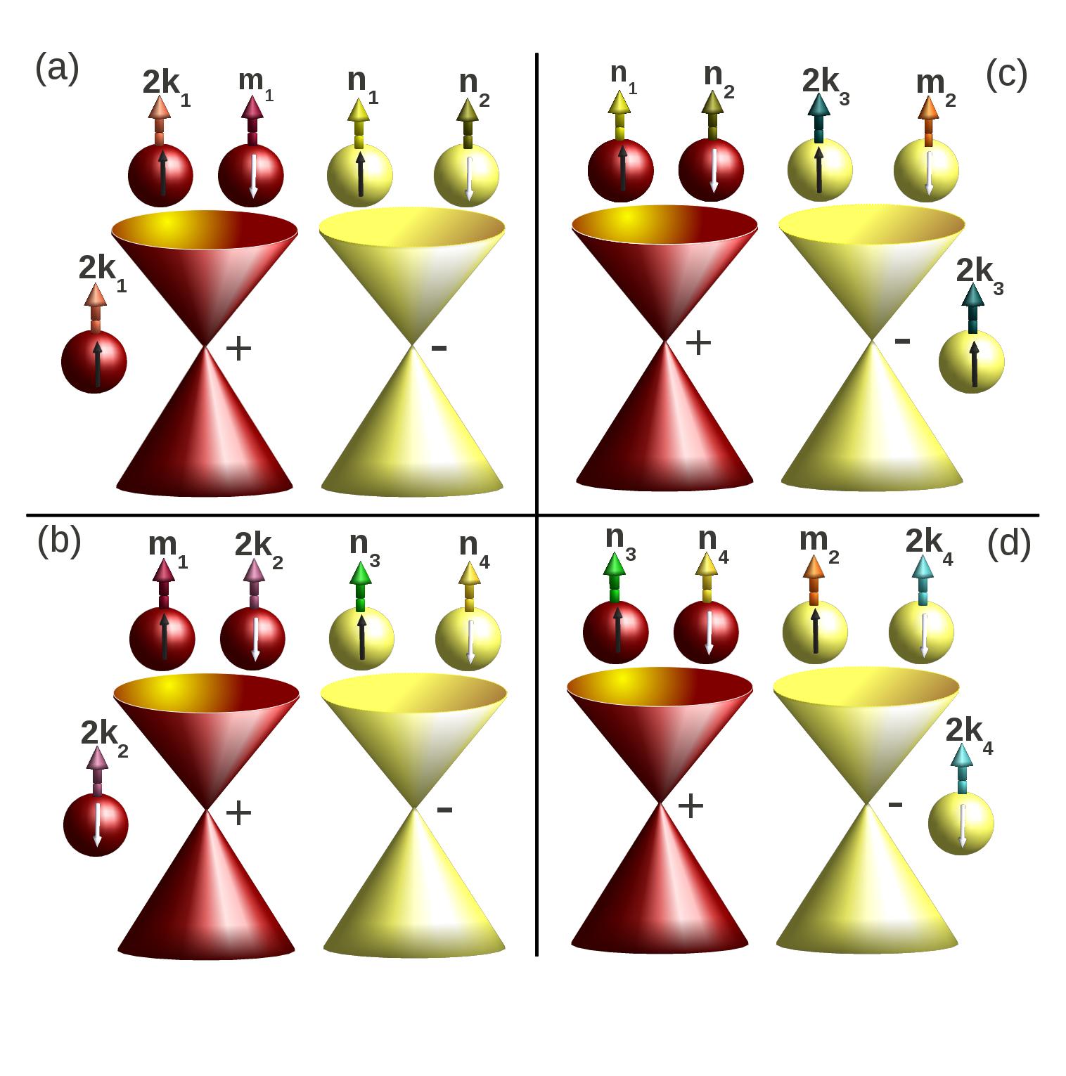
Figure 1: (color online) A pictorial representation of the flux attachment scheme. The two distinct Dirac cones in a single layer graphene are represented as $\pm$ valleys. The spheres represent electrons and their colors (identical to that of the Dirac cones) denote the valleys in which the electrons belong. The arrows pointing up(down) on the surface of the spheres represent the spins of the electrons. The thick arrows represent the flux attached to each electron. The number of flux quanta attached to each CS-CF with respective spin and valley are (a) $2k_{1}$ for $(\uparrow,+)$, (b) $2k_{2}$ for $(\downarrow,+)$, (c) $2k_{3}$ for $(\uparrow,-)$, and (d) $2k_{4}$ for $(\downarrow,-)$. The numbers written above the flux lines in each of the panels represent the number of flux quanta attached to the four different CS-CFs as seen by a (a) $(\uparrow,+)$, (b) $(\downarrow,+)$, (c) $(\uparrow,-)$, and (d) $(\downarrow,-)$ CS-CF.

We now introduce CS-CF quasiparticle creation operator $\psi^{\dagger}(\bm{r})$ in terms of $\psi_{e}^{\dagger}(\bm{r})$:

$$\psi^{\dagger}_{e,\alpha}(\bm{r})\rightarrow\psi_{\alpha}^{\dagger}(\bm{r})\exp\left[-i{\cal K}_{\alpha\beta}\int d\bm{r^{\prime}}\rm{arg}(\bm{r}-\bm{r^{\prime}})\rho_{\beta}(\bm{r^{\prime}})\right],$$ (3)

where the indices $\alpha$ and $\beta$ takes value from $1$ to $4$ described above and thus represents 4-components of the Dirac spinor in the spin and the valley space. Note that the CS transformation is a scalar in the pseudospin space and thus do not mix the sublattice indices of the electrons. Here $\rm{arg}(\bm{r}-\bm{r}^{\prime})$ represents the angle made by the vector $(\bm{r}-\bm{r}^{\prime})$ with x-axis and the explicit form of the matrix $\cal{K}$ is given by

$$\cal{K}=\left(\begin{array}[]{llll}2k_{1}&m_{1}&n_{1}&n_{2}\\ m_{1}&2k_{2}&n_{3}&n_{4}\\ n_{1}&n_{2}&2k_{3}&m_{2}\\ n_{3}&n_{4}&m_{2}&2k_{4}\end{array}\right),$$ (4)

where $k$’s, $m$’s and $n$’s are positive integers including zero. Note that the number of flux quanta attached to a CS-CF of species $\beta$ as seen by CS-CFs of species $\alpha$ is given by the component ${\cal K}_{\alpha\beta}$ (Eq. (4)). This is schematically shown in Fig. 1. The diagonal elements of ${\cal K}$ are chosen to be even integers so as to ensure the Fermionic statistics of the CS-CF quasiparticles.

Such a transformation leads to the effective Hamiltonian for the CS quasiparticles

$${\cal H}_{\rm{qp}} = \int d\bm{r}\psi_{\alpha}^{\dagger}(\bm{r})H_{\rm{eff}}\psi_{\alpha}(\bm{r})$$ (5)

$$+ \frac{1}{2}\int d\bm{r}\int d\bm{r}^{\prime}V(\bm{r}-\bm{r^{\prime}}):\hat{\rho}(\bm{r})\rho(\bm{r}^{\prime}):,$$

with

$$H_{\rm{eff}}=v_{F}\left(\begin{array}[]{cccc}\bm{\sigma}\cdot\bm{\tilde{\Pi}}_{1}&0&0&0\\ 0&\bm{\sigma}\cdot\bm{\tilde{\Pi}}_{2}&0&0\\ 0&0&(\bm{\sigma}\cdot\bm{\tilde{\Pi}}_{3})^{T}&0\\ 0&0&0&(\bm{\sigma}\cdot\bm{\tilde{\Pi}}_{4})^{T}\end{array}\right),$$ (6)

where $\bm{\tilde{\Pi}}_{\alpha}=-i\bm{\nabla}+e\bm{A}-\bm{a}_{\alpha}$. The 4-component CS gauge fields ${\bm{a}}_{\alpha}$ so obtained are given by

$$\bm{a}_{\alpha}={\cal K}_{\alpha\beta}\int d\bm{r}^{\prime}g(\bm{r}-\bm{r^{\prime}})\hat{\rho}_{\beta}(\bm{r^{\prime}}),$$ (7)

where $g(r)=(\hat{z}\times\bm{r})/r^{2}$. The corresponding 4-component CS magnetic fields are then given by

$$b_{\alpha}\equiv(1/e)\bm{\nabla}\times\bm{a}_{\alpha}=\phi_{0}{\cal K}_{\alpha\beta}\,\,\rho_{\beta}(\bm{r}).$$ (8)

Eq. 8 shows that each of the species of the CS-CF will experience different mean effective magnetic fields $B^{\ast}_{\alpha}$. The relation between these mean effective fields and the total applied physical field $B$ is given by

$$B^{*}_{\alpha}=B-\phi_{0}\cal{K}_{\alpha\beta}\,\,\rho_{\beta}.$$ (9)

where $\rho$’s are the mean densities. Note that $B^{*}_{\alpha}$ creates different set of effective Landau levels for the CS-CFs akin to Landau levels for electrons due to $B$. Denoting $\nu_{1}$, $\nu_{2}$, $\nu_{3}$, and $\nu_{4}$ be the number of effective Landau levels completely filled by the respective species of CS-CFs, one obtains the relation MR

$$\frac{\rho_{\alpha}}{\nu_{\alpha}}=\frac{\rho}{\nu}-\cal{K}_{\alpha\beta}\,\,\rho_{\beta}.$$ (10)

By defining the spin ($S$), the valley ($V$), and the mixed ($M$) polarizations respectively as

$$S = (\rho_{1}+\rho_{3}-\rho_{2}-\rho_{4})/\rho,$$

$$V = (\rho_{1}+\rho_{2}-\rho_{3}-\rho_{4})/\rho,$$

$$M = (\rho_{1}+\rho_{4}-\rho_{2}-\rho_{3})/\rho,$$ (11)

Eq. (10) can be expressed as

$$(1+S+V+M)(2k_{1}+\frac{1}{\nu_{1}})+(1+V-S-M)m_{1}$$

$$+(1-V)(n_{1}+n_{2})+(S-M)(n_{1}-n_{2})=\frac{4}{\nu},$$ (12)

$$(1-S+V-M)(2k_{2}+\frac{1}{\nu_{2}})+(1+V+S+M)m_{1}$$

$$+(1-V)(n_{3}+n_{4})+(S-M)(n_{3}-n_{4})=\frac{4}{\nu},$$ (13)

$$(1+S-V-M)(2k_{3}+\frac{1}{\nu_{3}})+(1-V-S+M)m_{2}$$

$$+(1+V)(n_{1}+n_{2})+(S+M)(n_{1}-n_{2})=\frac{4}{\nu},$$ (14)

$$(1-S-V+M)(2k_{4}+\frac{1}{\nu_{4}})+(1-V+S-M)m_{2}$$

$$+(1+V)(n_{3}+n_{4})+(S+M)(n_{3}-n_{4})=\frac{4}{\nu}.$$ (15)

Eqs. (12)..(15) represent the central result of this work and provide a relation between the total filling factor $\nu$ and the spin ($S$), the valley ($V$), and the mixed ($M$) polarizations of a FQHS in terms of the attached flux numbers $k$’s, $m$’s and $n$’s. The CS theory does not predict these attached flux numbers; however, one can use them as parameters whose variation leads to a list of possible FQHS at the saddle point level for a given $\nu$ with different values of $S$, $V$ and $M$. Thus the CS method do not predict a definite FQHS for a given filling $\nu$; it provides a list of possible FQHS. Moreover, in terms of these flux attachment numbers, one can write down, via a straightforward generalization of methods used in Refs. MR, ; LF2, , a variational wavefunction of these FQHS for the filling factor $\nu$ as

$$\Psi(u,v,w,z)={\cal P}_{L}\Phi_{\nu_{1}}(u_{1},\cdots,u_{N_{1}})\Phi_{\nu_{2}}(v_{1},\cdots,v_{N_{2}})$$

$$\times\Phi_{\nu_{3}}(w_{1},\cdots,w_{N_{3}})\Phi_{\nu_{4}}(z_{1},\cdots,z_{N_{4}})\prod_{i<j}^{N_{1}}(u_{i}-u_{j})^{2k_{1}}$$

$$\times\prod_{i<j}^{N_{2}}(v_{i}-v_{j})^{2k_{2}}\prod_{i<j}^{N_{3}}(w_{i}-w_{j})^{2k_{3}}\prod_{i<j}^{N_{4}}(z_{i}-z_{j})^{2k_{4}}$$

$$\times\prod_{i,j}^{N_{1},N_{2}}(u_{i}-v_{j})^{m_{1}}\prod_{i,j}^{N_{3},N_{4}}(w_{i}-z_{j})^{m_{2}}\prod_{i,j}^{N_{1},N_{3}}(u_{i}-w_{j})^{n_{1}}$$

$$\times\prod_{i,j}^{N_{1},N_{4}}(u_{i}-z_{j})^{n_{2}}\prod_{i,j}^{N_{2},N_{3}}(v_{i}-w_{j})^{n_{3}}\prod_{i,j}^{N_{2},N_{4}}(v_{i}-z_{j})^{n_{4}}$$

(16)

where $u$’s, $v$’s, $w$’s and $z$’s are complex coordinates for the particles of species $1$, $2$, $3$, and $4$ respectively laughlin1 , $N_{\alpha}$ denotes the number of CS-CFs of species $\alpha$, $\Phi_{\nu_{\alpha}}$ represents the IQHE wavefunction for $\nu_{\alpha}$ filled Landau levels of CS-CF belonging to species $\alpha$, and ${\cal P}_{L}$ represents projection into the LLL. We note here that the CS theory alone cannot lead to the wavefunction given in Eq. (16). Whereas the CS formalism does provide the exponents of both the inter- and intra-species Jastrow factors in Eq. (16), both the IQHE wavefunctions and the projection into the LLL receive input from the CF theory Jain . We expect the computation of the interaction energy of the system using Eq. (16) to provide further information about the FQHS in graphene. However, in this paper, instead of undertaking such a calculation, we shall be content to classify the possible FQHS based on Eqs. (12)..(15). We carry out this analysis in the next section.

III Filling factors and polarizations

In this section, we are going to address FQHS corresponding to specific value of the flux attachment parameters $\{k_{1},k_{2},k_{3},k_{4}\}$ and $\{m_{1},m_{2},n_{1},n_{2},n_{3},n_{4}\}$, and effective integer filling factors $\{\nu_{1},\nu_{2},\nu_{3},\nu_{4}\}$. While Eqs. (12)..(15) may be used to determine $\nu$, $S$, $V$ and $M$ for any set of parameters (except $M$, $S$ or $V$ may remain undetermined for some special cases which we shall discuss below), in the rest of this work, we focus on some specific choices of these parameters which allow simple analytical solution to these equations. More specifically, we choose the flux seen by inter-valley CS-CFs and the flux attached to each CS-CF to be independent of their spin. This imposes the restriction $n_{1}=n_{2}=n_{3}=n_{4}=n$ and $k_{1}=k_{2},\,k_{3}=k_{4}$. Within this restricted parameter space, we find analytical solutions to Eqs. (12)..(15) and discuss several possible FQHS which arise out of these solutions. We arrange these solutions into several distinct groups below.

I. Arbitrary values of $\nu_{1},\nu_{2},\nu_{3}$ and $\nu_{4}$ :

(a) $2k_{1}=2k_{3}=m_{1}=m_{2}=n=2k$: In this case, all the matrix elements of ${\cal K}$ have the same value since the number of flux quanta attached to each CS-CFs and as seen by other CS-CFs, irrespective of the species of CS-CFs, are $2k$. The eigenvalues of ${\cal K}$ matrix for this special case are $8k$ and $0$ (triply degenerate). Therefore there is only one dynamical CS gauge field ${\cal A}^{\mu}=a^{\mu}_{1}+a^{\mu}_{2}+a^{\mu}_{3}+a^{\mu}_{4}$. The rest of the CS gauge fields decouple MR . Solving Eq. (12)..(15), we find

$$\nu = \frac{\nu^{*}}{2k\nu^{*}+1}\,,\,V=\frac{2(\nu_{1}+\nu_{2})-\nu^{*}}{\nu^{*}},$$

$$S = \frac{2(\nu_{1}+\nu_{3})-\nu^{*}}{\nu^{*}}\,,\,M=\frac{2(\nu_{1}+\nu_{4})-\nu^{*}}{\nu^{*}},$$ (17)

where $\nu^{*}=\nu_{1}+\nu_{2}+\nu_{3}+\nu_{4}$. This is precisely the Toke-Jain sequence in graphene CF2 and the wavefunction [Eq. (16)] obtained for these set of parameters exactly matches with the CF wave function CF2 . The sequence of FQHS generated with this set of parameters is same as the SU(2) sequence for $\nu^{*}\leq 2$. We note that these states can be degenerate. For example, for $\nu^{*}=2$, the two effective Landau levels may be filled by two different species of CS-CFs, leading to a six-fold degeneracy of the ground state. We find that in the limit $\nu^{*}\to\infty$, $\nu=1/2k$ and hence these even denominator states correspond to Fermi sea of CFs HLR .

We note that the class of solutions [Eq. (17)] which has equal exponents in the Jastrow factors in their wavefunction as can be seen from Eq. (16). However, the CF wave function for bilayers, constructed in Ref. Scarola, , do not necessarily have equal exponents in Jastrow factors for intra- and inter-layer CFs. Taking cue from this, we now construct solutions to Eqs. (12)..(15) where the off-diagonal elements of ${\cal K}$ are different from the diagonal elements. We discuss these solutions as cases (b), and (c) below.

(b) $2k_{1}=2k_{3}=m_{1}=m_{2}=2k$ and $n\neq 2k$: For this choice of parameters, we find

$$\nu = \frac{\nu^{*}+2(2k-n)(\nu_{1}+\nu_{2})(\nu_{3}+\nu_{4})}{2k\nu^{*}+1+(4k^{2}-n^{2})(\nu_{1}+\nu_{2})(\nu_{3}+\nu_{4})},$$

$$V = \frac{2(\nu_{1}+\nu_{2})-\nu^{*}}{\nu^{*}+2(2k-n)(\nu_{1}+\nu_{2})(\nu_{3}+\nu_{4})},$$

$$S = \frac{2(\nu_{1}+\nu_{3})-\nu^{*}+2(2k-n)(\nu_{1}\nu_{3}-\nu_{2}\nu_{4})}{\nu^{*}+2(2k-n)(\nu_{1}+\nu_{2})(\nu_{3}+\nu_{4})},$$

$$M = \frac{2(\nu_{1}+\nu_{4})-\nu^{*}+2(2k-n)(\nu_{1}\nu_{4}-\nu_{2}\nu_{3})}{\nu^{*}+2(2k-n)(\nu_{1}+\nu_{2})(\nu_{3}+\nu_{4})}.$$ (18)

Note that for these solutions, the even denominator FQHS with $\nu=1/2k$ occurs when $(2k-n)^{2}=1/[(\nu_{1}+\nu_{2})(\nu_{3}+\nu_{4})]$. Since $k$, $n$, and $\nu$’s are integers, the only possible way to satisfy this condition is to have $(\nu_{1}+\nu_{2})=1=(\nu_{3}+\nu_{4})$ and $n=2k\pm 1$. We point out that the even-denominator FQHS so obtained do not correspond to $\nu^{\ast}\to\infty$ and hence do not lead to the formation of a Fermi sea of CS-CF. These states are similar to those obtained for bilayer SU(2) quantum Hall systems.

(c) $2k_{1}=2k_{3}=2k$, $m_{1}=m_{2}=m\neq 2k$, and $n\neq 2k$: In this case, we find solutions with zero spin and mixed polarization ($M=S=0$) and with finite non-zero valley polarizations given by

$$\nu = \left[4\nu^{*}+4(2k+m-2n)(\nu_{1}+\nu_{2})(\nu_{3}+\nu_{4})\right]/{\mathcal{D}},$$

$${\mathcal{D}} = 4+2(2k+m)\nu^{*}+((2k+m)^{2}-4n^{2})$$

$$\times(\nu_{1}+\nu_{2})(\nu_{3}+\nu_{4}),$$

$$V = \frac{2(\nu_{1}+\nu_{2})-\nu^{*}}{2\nu^{*}+2(2k+m-2n)(\nu_{1}+\nu_{2})(\nu_{3}+\nu_{4})}.$$ (19)

We note that these states do not have any analogue in U(1) and SU(2) FQHE and can only occur for SU(4) symmetric FQHE. Similarly, a set of FQHS can be found, again for $2k_{1}=2k_{3}=2k$, $m_{1}=m_{2}=m$, and $n\neq 2k$, where the mixed and the valley polarizations vanish ($M=V=0$), but the spin polarization $S$ remain finite. These states correspond to

$$\nu = \frac{4(\nu_{2}\nu_{3}-\nu_{1}\nu_{4})}{\nu^{*}-2(\nu_{1}+\nu_{4})+(2k+m+2n)(\nu_{2}\nu_{3}-\nu_{1}\nu_{4})},$$

$$S = \frac{\nu^{*}-2(\nu_{1}+\nu_{2})}{(2k-m)(\nu_{2}\nu_{3}-\nu_{1}\nu_{4})}.$$ (20)

The same choice of parameters also allows for FQHS with $S=V=0$ and finite $M$ which are given by

$$\nu = \frac{4(\nu_{1}\nu_{3}-\nu_{2}\nu_{4})}{\nu^{*}-2(\nu_{2}+\nu_{4})+(2k+m+2n)(\nu_{1}\nu_{3}-\nu_{2}\nu_{4})},$$

$$M = \frac{2(\nu_{1}+\nu_{2})-\nu^{*}}{(2k-m)(\nu_{1}\nu_{3}-\nu_{2}\nu_{4})}.$$ (21)

Note that none of the above-mentioned states have any analogue in U(1) and SU(2) FQHS.

II. SU(4) singlet case: $\nu_{1}=\nu_{2}=\nu_{3}=\nu_{4}=1$

For the SU(4) singlet states which correspond to all $\nu_{i}=1$, one has several possible solutions. The filling factors for these class of solutions which correspond to zero spin, valley and mixed polarizations ($M=S=V=0$) are given by

$$\nu=\frac{8}{2+2k_{1}+2k_{3}+m_{1}+m_{2}+4n}$$ (22)

provided that $2k_{1}+1\neq m_{1}$ and $2k_{3}+1\neq m_{2}$. Below, we classify the other SU(4) singlet FQHS.

The first such set of states that we classify consists of $M=S=0$ but $V\neq 0$. These FQHS correspond to

$$\nu = \frac{4(1+k_{1}+k_{3})+2(m_{1}+m_{2}-4n)}{(2k_{1}+1+m_{1})(2k_{3}+1+m_{2})-4n^{2}},$$ (23)

$$V = \frac{2(k_{3}-k_{1})+m_{2}-m_{1}}{2(1+k_{1}+k_{3})+(m_{1}+m_{2}-4n)},$$ (24)

and have finite valley but no spin and mixed polarization.

The second class of states correspond to $k_{1}=k_{3}=k$. First, we note that for these states, if we choose $2k+1=m_{1}=m_{2}=m$, we find that

$$\nu=\frac{2}{m+n},$$ (25)

For these states, $M$ and $S$ are undetermined. $V$ can be determined only if $m\neq n$ ( which correspond to $V$=0); for $m=n$, $V$ is also undetermined. The filling factors for these states with $V=0$ are $2/3$, $1/2$, and $2/5$ for $k=1$ and $2/5$, $1/3$, $2/7$, $1/4$, and $2/9$ for $k=2$. In contrast, the states for which $V$ is also undetermined have filling factor $1/3$ with $k=1$ and $1/5$ with $k=2$. The wavefunctions [Eq. (16)] for the filling factors $2/3$, $2/5$, and $1/3$ obtained from our formalism are precisely the same Halperin-like wavefunctions proposed in Ref. Regnault, . We note that the even denominator states in the above-mentioned sequence (such as $1/2$ and $1/4$) do not correspond to the Fermi sea of CFs. Second, if $2k+1=m_{1}\neq m_{2}$, the solutions of Eqs. (12)..(15) yields FQHS with $M=S$ but undetermined, and with the values of the filling fractions and the valley polarizations given by

$$\nu=\frac{3m_{1}+m_{2}-4n}{m_{1}^{2}+m_{1}m_{2}-2n^{2}}\,,V=\frac{m_{2}-m_{1}}{3m_{1}+m_{2}-4n}.$$ (26)

These states do not appear in the work of Ref. Regnault, . Similar states with undetermined $M$ and $S$ and with $M=S$ also occurs for $k_{1}\neq k_{3}$, and $2k_{1}+1=m_{1}=m_{2}=m$. The corresponding filling fractions and valley polarizations are given by

$$\nu=\frac{2k_{3}+1+3m-4n}{(2k_{3}+1+m)m-2n^{2}},V=\frac{2k_{3}+1-m}{2k_{3}+1+3m-4n}.$$ (27)

Finally, we note that if one chooses $2k_{1}+1=m_{1}$ and $2k_{3}+1=m_{2}$, one finds FQHS with $M$ and $S$ undetermined but not necessarily equal which yields

$$\nu=\frac{m_{1}+m_{2}-2n}{m_{1}m_{2}-n^{2}}\,,V=\frac{m_{2}-m_{1}}{m_{1}+m_{2}-2n}\,.$$ (28)

The filling factors for all the SU(4) singlet FQHS and their corresponding spin, valley and mixed polarizations are tabulated in Tables 1 and 2. We point out that these states constitutes the simplest possible FQHS in monolayer graphene which do not have any analogue in U(1) and SU(2) FQHE. We note that the same states would show up in spin polarized bilayer graphene when $S$ is interpreted as layer polarization and in quantum Hall bilayer system where $V$ is interpreted as the layer polarization. Further the filling factors for some of these FQHS, such as $8/19$, are only found for SU(4) case Regnault . It is interesting to observe that FQHS with filling factor $2/3$ and $3/5$ can be obtained only by attaching antiparallel flux to the CFs in CF theory Jain ; CF1 ; CF2 . In contrast, the CS analysis suggests these states may also arise due to parallel flux attachment as seen from Tables 1 and 2 . Also, while FQHS with filling factor $\nu=4/11$ correspond to FQHE of CFs in U(1) or SU(2) CF theoryMJ ; CMJ , it may arise due to IQHE of CS-CFs in SU(4) FQHE. Finally, we note that the general formulae provided in Eqs. (12)..(15) may contain many other FQHS. A detailed numerical analysis of these states is left for future study.

IV Conclusion

In summary, we have developed a Fermionic CS theory for SU(4) FQHE and analyzed the possible FQHS obtained from such a theory. We have reproduced SU(4) FQHS arising from CF theory CF2 as well as Halperin-like Regnault states within a single unified formalism. We have also proposed several other states which are not obtained in the previous studies. Although the filling factors and their polarizations presented here are for monolayer graphene, the analysis is valid for any SU(4) system. Two other examples of such systems where this theory could be applicable are bilayer quantum Hall systems and bilayer graphene Nomura with complete spin or valley polarizations. Taking cue from the CS theory Jain , we have proposed wavefunctions for all of these FQHS. We note that for FQHS with particular filling factor, the precise ground state wavefunction will depend on the exact nature of the interaction between electrons. It will be interesting to obtain the overlap of the ground state with our proposed wavefunction. Finally, the ground state for FQHS in graphene may be tuned by tuning either the Zeeman coupling or the inter-valley coupling. It will certainly be interesting to use our proposed wavefunction to study the resulting transitions between the FQHS for all of these states by changing Zeeman coupling and obtain the corresponding phase diagram. We leave these issues for future studies.

KS thanks DST for support through grant SR/S2/CMP-001/2009.

Table 1: A chart of the possible filling fractions $\nu$ with numerator $<5$ for the SU(4) singlet states and the corresponding polarizations $S$, $V$ and $M$ for different sets of parameters $\{k_{1},k_{3},m_{1},m_{2},n\}$. Here we have chosen $k_{1}=k_{2}$, $k_{3}=k_{4}$, $\nu_{1}=\nu_{2}=\nu_{3}=\nu_{4}=1$, $k_{3}=1,2$, $k_{1}\leq k_{3}$, $m_{1}\leq 2k_{1}+1$, $m_{2}\leq 2k_{3}+1$, and $n=0$.. max($m_{1},m_{2}$). The symbol ‘–’ for the polarizations denotes undetermined value. In the last column, we tabulate the Eq. number from which the corresponding state has been computed.

$\,\,\nu\,\,$	$\,\,k_{1}\,\,$	$\,\,k_{3}\,\,$	$\,\,m_{1}\,\,$	$\,\,m_{2}\,\,$	$\,\,n\,\,$	$\,\,S\,\,$	$\,\,V\,\,$	$\,\,M\,\,$	Eq. No.
$1/2$	1	1	3	3	1	–	0	–	(25)
$1/2$	1	2	2	3	1	0	1/3	0	(23-24)
$1/2$	2	2	0	3	1	0	1/3	0	(23-24)
$1/2$	2	2	1	1	1	0	0	0	(22)
$1/2$	2	2	3	3	0	0	0	0	(22)
$1/3$	1	1	3	3	3	–	–	–	(25)
$1/3$	2	2	5	5	1	–	0	–	(25)
$1/4$	2	2	5	5	3	–	0	–	(25)
$1/5$	2	2	5	5	5	–	–	–	(25)
$2/3$	1	1	1	1	1	0	0	0	(22)
$2/3$	1	1	3	3	0	–	0	–	(25)
$2/3$	2	2	1	1	0	0	0	0	(22)
$2/5$	1	1	3	3	2	–	0	–	(25)
$2/5$	2	2	5	5	0	–	0	–	(25)
$2/5$	2	2	3	3	1	0	0	0	(22)
$2/7$	2	2	3	3	3	0	0	0	(22)
$2/7$	2	2	5	5	2	–	0	–	(22)
$2/9$	2	2	5	5	4	–	0	–	(25)
$3/4$	1	1	0	1	1	0	1/3	0	(23-24)
$3/4$	1	2	1	3	0	0	1/3	0	(23-24)
$3/5$	1	2	1	1	1	0	1/3	0	(23-24)
$3/7$	1	2	2	1	2	0	1/3	0	(23-24)
$3/7$	1	2	3	5	1	–	1/3	–	(28)
$3/8$	1	2	3	3	2	–	1/3	–	(27)
$3/8$	2	2	1	3	2	0	1/3	0	(23-24)
$4/5$	1	1	2	2	0	0	0	0	(22)
$4/5$	1	2	2	0	0	0	0	0	(22)
$4/5$	2	2	0	0	0	0	0	0	(22)
$4/7$	1	1	2	2	1	0	0	0	(22)
$4/7$	1	2	1	3	1	0	1/2	0	(23-24)
$4/7$	1	2	2	0	1	0	0	0	(22)
$4/7$	2	2	2	2	0	0	0	0	(22)
$4/9$	1	1	2	2	2	0	0	0	(22)
$4/9$	1	2	2	0	2	0	0	0	(22)
$4/9$	2	2	2	2	1	0	0	0	(22)
$4/9$	2	2	4	4	0	0	0	0	(22)
$4/11$	1	2	3	5	2	–	1/2	–	(28)
$4/11$	2	2	2	2	2	0	0	0	(22)
$4/11$	2	2	4	4	1	0	0	0	(22)
$4/13$	2	2	4	4	2	0	0	0	(22)
$4/15$	2	2	4	4	3	0	0	0	(22)
$4/17$	2	2	4	4	4	0	0	0	(22)

Table 2: Same as in Table 1 but with numerators $\geq 5$.

$\,\,\nu\,\,$	$\,\,k_{1}\,\,$	$\,\,k_{3}\,\,$	$\,\,m_{1}\,\,$	$\,\,m_{2}\,\,$	$\,\,n\,\,$	$\,\,S\,\,$	$\,\,V\,\,$	$\,\,M\,\,$	Eq. No.
$5/6$	1	2	1	1	0	0	1/5	0	(23-24)
$5/7$	1	2	0	1	1	0	3/5	0	(23-24)
$5/8$	1	1	1	2	1	0	1/5	0	(23-24)
$5/8$	1	2	1	0	1	0	1/2	0	(23-24)
$5/9$	2	2	1	4	0	0	1/5	0	(23-24)
$5/12$	1	2	2	3	2	0	3/5	0	(23-24)
$5/12$	2	2	0	3	2	0	3/5	0	(23-24)
$5/13$	2	2	1	2	2	0	1/5	0	(23-24)
$5/18$	2	2	3	4	3	0	1/5	0	(23-24)
$7/10$	1	2	0	3	1	0	5/7	0	(23-24)
$7/12$	1	2	1	2	1	0	3/7	0	(23-24)
$7/12$	1	2	3	3	0	–	1/7	–	(27)
$7/12$	2	2	1	3	0	0	1/7	0	(23-24)
$7/13$	1	2	2	1	1	0	1/7	0	(23-24)
$7/13$	2	2	0	1	1	0	1/7	0	(23-24)
$7/19$	2	2	1	4	2	0	3/7	0	(23-24)
$8/9$	1	2	0	4	0	0	1/2	0	(23-24)
$8/11$	1	1	0	2	1	0	1/2	0	(23-24)
$8/19$	1	2	2	2	2	0	1/2	0	(23-24)
$8/19$	2	2	0	2	2	0	1/2	0	(23-24)

References

- (1) D. C. Tsui, H. L. Stormer, and A. C. Gossard, Phys. Rev. Lett. 48, 1559 (1982).
- (2) R. B. Laughlin, Phys. Rev. Lett. 50, 1395 (1983).
- (3) J. K. Jain, Phys. Rev. Lett. 63, 199 (1989).
- (4) A. Lopez and E. Fradkin, Phys. Rev. B 44, 5246 (1991).
- (5) B. I. Halperin, P. A. Lee and N. Read, Phys. Rev. B 47, 7312 (1993).
- (6) S. S . Mandal and V. Ravishankar, Phys. Rev. B 54, 8688 (1996).
- (7) A. Lopez and E. Fradkin, Phys. Rev. B 51, 4347 (1995).
- (8) K. S. Novoselov, A. K. Geim, S. V. Morozov, D. Jiang, M. I. Katesnelson, I. V. Grigoreva, S. V. Dubonos, and A. Firsov, Nature 438, 197 (2005).
- (9) Y. B. Zhang, Y. W. Tan, H. L. Stormer, and P. Kim, Nature 438, 201 (2005).
- (10) X. Du, I. Shachko, F. Duerr, A. Luican, E. Y. Andrei, Nature 462, 192 (2009).
- (11) K. I. Bolotin, F. Ghahari, M. D. Shulman, H. L. Stormer, and P. Kim, Nature 462, 196 (2009).
- (12) F. Ghahari, Y. Zhao, P. C.-Zimansky, K. Bolotin, and P. Kim, arXiv:1010.1187.
- (13) A. H. Castro Neto, F. Guinea, N. M. R. Peres, K. S. Novoselov, and A. K. Geim, Rev. Mod. Phys. 81, 109 (2009).
- (14) C. Toke, P. E. Lammert, V. H. Crespi, and J. K. Jain, Phys. Rev. B 74, 235417 (2006).
- (15) V. M. Apalkov and T. Chakraborty, Phys. Rev. Lett. 97, 126801 (2006).
- (16) C. Toke and J. K. Jain, Phys. Rev, B 75, 245440 (2007).
- (17) M. O. Goerbig and N. Regnault, Phys. Rev. B 75, 241405 (2007).
- (18) D. V. Khveshchenko, Phys. Rev. B 75, 153405 (2007).
- (19) V. W. Scarola and J. K. Jain, Phys. Rev. B 64, 085313 (2001).
- (20) S. S. Mandal and J. K. Jain, Phys. Rev. B 66, 155302 (2002).
- (21) C. C. Chang, S. S. Mandal, and J. K. Jain, Phys. Rev. B 67, 121305(R) (2003).
- (22) V. W. Scarola and J. K. Jain, Phys. Rev. B 64, 085313 (2001).
- (23) N. Shibata and K. Nomura, arXiv:0906.1037 (unpublished).