The geometry of spontaneous spiking in neuronal networks
Abstract
The mathematical theory of pattern formation in electrically coupled networks of excitable neurons forced by small noise is presented in this work. Using the Freidlin-Wentzell large deviation theory for randomly perturbed dynamical systems and the elements of the algebraic graph theory, we identify and analyze the main regimes in the network dynamics in terms of the key control parameters: excitability, coupling strength, and network topology. The analysis reveals the geometry of spontaneous dynamics in electrically coupled network. Specifically, we show that the location of the minima of a certain continuous function on the surface of the unit cube encodes the most likely activity patterns generated by the network. By studying how the minima of this function evolve under the variation of the coupling strength, we describe the principal transformations in the network dynamics. The minimization problem is also used for the quantitative description of the main dynamical regimes and transitions between them. In particular, for the weak and strong coupling regimes, we present asymptotic formulae for the network activity rate as a function of the coupling strength and the degree of the network. The variational analysis is complemented by the stability analysis of the synchronous state in the strong coupling regime. The stability estimates reveal the contribution of the network connectivity and the properties of the cycle subspace associated with the graph of the network to its synchronization properties. This work is motivated by the experimental and modeling studies of the ensemble of neurons in the Locus Coeruleus, a nucleus in the brainstem involved in the regulation of cognitive performance and behavior.
1 Introduction
Direct electrical coupling through gap-junctions is a common way of communication between neurons, as well as between cells of the heart, pancreas, and other physiological systems [10]. Electrical synapses are important for synchronization of the network activity, wave propagation, and pattern formation in neuronal networks. A prominent example of a gap-junctionally coupled network, whose dynamics is thought to be important for cognitive processing, is a group of neurons in the Locus Coeruleus (LC), a nucleus in the brainstem [1, 4, 37]. Electrophysiological studies of the animals performing a visual discrimination test show that the rate and the pattern of activity of the LC network correlate with the cognitive performance [38]. Specifically, the periods of the high spontaneous activity correspond to the periods of poor performance, whereas the periods of low synchronized activity coincide with good performance. Based on the physiological properties of the LC network, it was proposed that the transitions between the periods of high and low network activity are due to the variations in the strength of coupling between the LC neurons [38]. This hypothesis motivates the following dynamical problem: to study how the dynamics of electrically coupled networks depends on the coupling strength. This question is the focus of the present work.
The dynamics of an electrically coupled network depends on the properties of the attractors of the local dynamical systems and the interactions between them. Following [38], we assume that the individual neurons in the LC network are spontaneously active. Specifically, we model them with excitable dynamical systems forced by small noise. We show that depending on the strength of electrical coupling, there are three main regimes of the network dynamics: uncorrelated spontaneous firing (weak coupling), formation of clusters and waves (intermediate coupling), and synchrony (strong coupling). The qualitative features of these regimes are independent from the details of the models of the individual neurons and network topology. Using the center manifold reduction [8, 18] and the Freidlin-Wentzell large deviation theory [14], we derive a variational problem, which provides a useful geometric interpretation for various patterns of spontaneous activity. Specifically, we show that the location of the minima of a certain continuous function on the surface of the unit cube encodes the most likely activity patterns generated by the network. By studying the evolution of the minima of this function under the variation of the control parameter (coupling strength), we identify the principal transformations in the network dynamics. The minimization problem is also used for the quantitative description of the main dynamical regimes and transitions between them. In particular, for the weak and strong coupling regimes, we present asymptotic formulae for the activity rate as a function of the coupling strength and the degree of the network. The variational analysis is complemented by the stability analysis of the synchronous state in the strong coupling regime. In analyzing various aspects of the network dynamics, we pay special attention to the role of the structural properties of the network in shaping its dynamics. We show that in weakly coupled networks, only very rough structural properties of the underlying graph matter, whereas in the strong coupling regime, the finer features, such as the algebraic connectivity and the properties of the cycle subspace associated with the graph of the network, become important. Therefore, this paper presents a comprehensive analysis of electrically coupled networks of excitable cells in the presence of noise. It complements the existing studies of related deterministic networks of electrically coupled oscillators (see, e.g., [11, 19, 26, 33] and references therein).
The outline of the paper is as follows. In Section 2, we formulate the biophysical model of the LC network. Section 3 presents numerical experiments elucidating the principal features of the network dynamics. In Section 4, we reformulate the problem in terms of the bifurcation properties of the local dynamical systems and the properties of the linear coupling operator. We then introduce the variational problem, whose analysis explains the main dynamical regimes of the coupled system. In Section 5, we analyze the stability of the synchronous dynamics in the strong coupling regime, using fast-slow decomposition. The results of this work are summarized in Section 6.
2 The model
2.1 The single cell model
According to the dynamical mechanism underlying action potential generation, conductance-based models of neurons are divided into Type I and Type II classes [35]. The former assumes that the model is near the saddle-node bifurcation, while the latter is based on the Andronov-Hopf bifurcation. Electrophysiological recordings of the LC neurons exhibit features that are consistent with the Type I excitability. The existing biophysical models of LC neurons use Type I action potential generating mechanism [2, 5]. In accord with these experimental and modeling studies, we use a generic Type I conductance-based model to simulate the dynamics of the individual LC neuron
| (2.1) | |||||
| (2.2) |
Here, dynamical variables and are the membrane potential and the activation of the potassium current, , respectively. stands for the membrane capacitance. The ionic currents are modeled using the Hodgkin-Huxley formalism (see Appendix for the definitions of the functions and parameter values used in (2.1) and (2.2)). A small Gaussian white noise is added to the right hand side of (2.1) to simulate random synaptic input and other possible fluctuations affecting system’s dynamics. Without noise (), the system is in the excitable regime. For , it exhibits spontaneous spiking. The frequency of the spontaneous firing depends on the proximity of the deterministic system to the saddle-node bifurcation and on the noise intensity. A typical trajectory of (2.1) and (2.2) stays in a small neighborhood of the stable equilibrium most of the time (Fig. 1a). Occasionally, it leaves the vicinity of the fixed point to make a large excursion in the phase plane and then returns to the neighborhood of the steady state (Fig. 1a). These dynamics generate a train of random spikes in the voltage time series (Fig. 1b).
a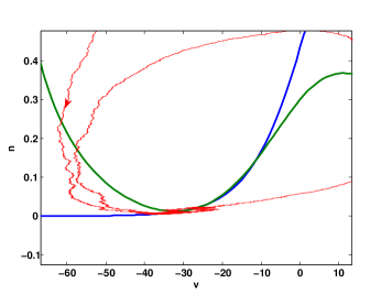 b
b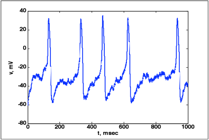
In neuroscience, the (average) firing rate provides a convenient measure of activity of neural cells and neuronal populations. It is important to know how the firing rate depends on the parameters of the model. In this paper, we study the factors determining the rate of firing in electrically coupled network of neurons. However, before setting out to study the network dynamics, it is instructive to discuss the behavior of the single neuron model first. To this end, we use the center-manifold reduction to approximate (2.1) and (2.2) by a system:
| (2.3) |
where is the rescaled projection of onto a slow manifold, is the distance to the saddle-node bifurcation, and is the noise intensity after rescaling. We postpone the details of the center-manifold reduction until we analyze a more general network model in §4.1.
The time between two successive spikes in voltage time series corresponds to the first time the trajectory of (2.3) with initial condition overcomes potential barrier . The large deviation estimates (cf. [14]) yield the logarithmic asymptotics of the first crossing time
| (2.4) |
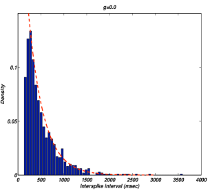
where stands for the expected value with respect to the probability generated by the random process with initial condition . Throughout this paper, we use to denote logarithmic asymptotics. It is also known that the first exit time is distributed exponentially as shown in Fig. 2 (cf. [12]).
Equation (2.4) implies that the statistics of spontaneous spiking of a single cell is determined by the distance of the neuronal model (2.1) and (2.2) to the saddle-node bifurcation and the intensity of noise. Below we show that, in addition to these two parameters, the strength and topology of coupling are important factors determining the firing rate of the coupled population.
2.2 The electrically coupled network
The network model includes cells, whose intrinsic dynamics is defined by (2.1) and (2.2), coupled by gap-junctions. The gap-junctional current that Cell receives from the other cells in the network is given by
| (2.5) |
where is the gap-junction conductance and
Adjacency matrix defines the network connectivity. By adding the coupling current to the right hand side of the voltage equation (2.1) and combining the equations for all neurons in the network, we arrive at the following model
| (2.6) | |||||
| (2.7) |
where are independent copies of the standard Brownian motion.
a b
b c
c
The network topology is an important parameter of the model (2.6) and (2.7). The following terminology and constructions from the algebraic graph theory [6] will be useful for studying the role of the network structure in shaping its dynamics. Let denote the graph of interactions between the cells in the network. Here, and denote the sets of vertices (i.e., cells) and edges (i.e., the pairs of connected cells), respectively. Throughout this paper, we assume that is a connected graph. For each edge , we declare one of the vertices to be the positive end (head) of , and the other to be the negative end (tail). Thus, we assign an orientation to each edge from its tail to its head. The coboundary matrix of is defined as follows (cf. [6])
| (2.8) |
Let be a spanning tree of , i.e., a connected subgraph of such that , and there are no cycles in [6]. Without loss of generality, we assume that
| (2.9) |
Denote the coboundary matrix of by .
Matrix
| (2.10) |
is called a graph Laplacian of . The Laplacian is independent of the choice of orientation of edges that was used in the definition of [6]. Alternatively, the Laplacian can be defined as
| (2.11) |
where is the degree map and is the adjacency matrix of .
Let
denote the eigenvalues of arranged in the increasing order counting the multiplicity. The spectrum of the graph Laplacian captures many structural properties of the network (cf. [6, 7, 9]). In particular, the first eigenvalue of , , is simple if and only if the graph is connected [16]. The second eigenvalue is called the algebraic connectivity of , because it yields a lower bound for the edge and the vertex connectivity of [16]. The algebraic connectivity is important for a variety of combinatorial, probabilistic, and dynamical aspects of the network analysis. In particular, it is used in the studies of the graph expansion [22], random walks [7], and synchronization of dynamical networks [17, 29].
Next, we introduce several examples of the network connectivity including nearest neighbor arrays of varying degree and a pair of degree symmetric and random graphs. These examples will be used to illustrate the role of the network topology in pattern formation.
a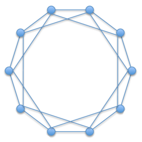 b
b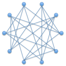
Example 2.1.
The nearest-neighbor coupling scheme is an example of the local connectivity (Fig. 3a). For simplicity, we consider a array. For higher dimensional lattices, the nearest neighbor coupling is defined similarly. In this configuration, each cell in the interior of the array is coupled to two nearest neighbors. This leads to the following expression for the coupling current:
The coupling currents for the cells on the boundary are given by
The corresponding graph Laplacian is
| (2.12) |
Example 2.2.
The nearest neighbor coupling scheme is a natural generalization of the previous example. Suppose each cell is coupled to of its nearest neighbors from each side whenever they exist or as many as possible otherwise:
| (2.13) |
where we use a customary convention that if . The coupling matrix can be easily derived from (2.13).
Example 2.3.
The all-to-all coupling features global connectivity (Fig. 3c):
| (2.14) |
The Laplacian in this case has the following form
| (2.15) |
The graphs in the previous examples have different degrees: ranging from in Example 2.1 to in Example 2.3. In addition to the degree of the graph, the pattern of connectivity itself is important for the network dynamics. This motivates our next example.
Example 2.4.
Graphs with random connections like the one in the last example represent expanders, a class of graphs used in many important applications in mathematics, computer science and other branches of science and technology (cf. [22]). In Section 5 we show that dynamical networks on expanders have very good synchronization properties (see also [29]).
Example 2.5.
Let be a family of graphs on vertices, with the following property:
| (2.16) |
Such graphs are called (spectral) expanders [22, 36]. There are known explicit constructions of expanders, including the celebrated Ramanujan graphs [28, 27]. In addition, families of random graphs have good expansion properties. In particular, it is known that
| (2.17) |
where stands for the family of random graphs of degree and [15].
a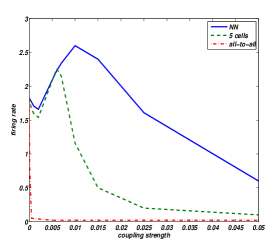 b
b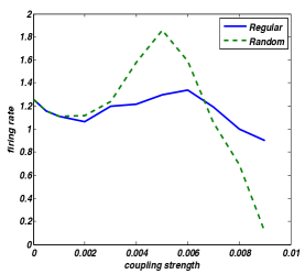 c
c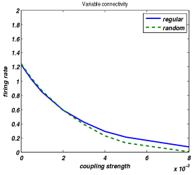
3 Numerical experiments
The four parameters controlling the dynamics of the biophysical model (2.6) and (2.7) are the excitability, the noise intensity, the coupling strength, and the network topology. Assuming that the system is at a fixed distance from the bifurcation, we study the dynamics of the coupled system for sufficiently small noise intensity . Therefore, the two remaining parameters are the coupling strength and the network topology. We focus on the impact of the coupling strength on the spontaneous dynamics first. At the end of this section, we discuss the role of the network topology. The numerical experiments of this section show that activity patterns generated by the network are effectively controlled by the variations of the coupling strength.
a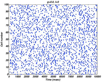 b
b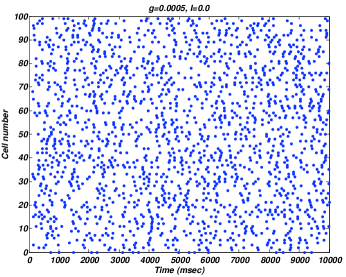 c
c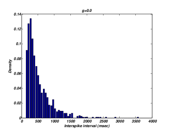 d
d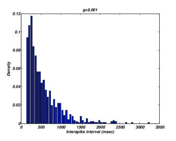
3.1 Three phases of spontaneous activity
To measure the activity of the network for different values of the control parameters, we will use the average firing rate - the number of spikes generated by the network per one neuron and per unit time. Fig. 5a shows that the activity rate varies significantly with the coupling strength. The three intervals of monotonicity of the activity rate plot reflect three main stages in the network dynamics en route to complete synchrony: weakly correlated spontaneous spiking, formation of clusters and wave propagation, and synchronization. We discuss these regimes in more detail below.
a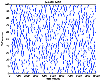 b
b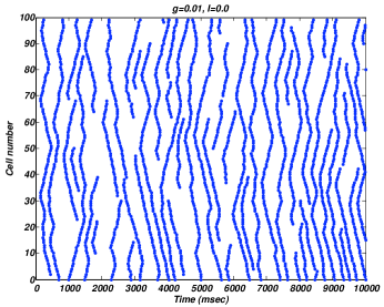 c
c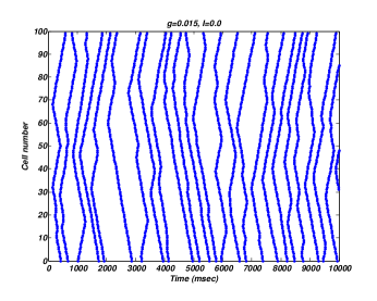 d
d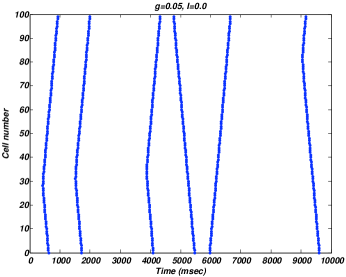
a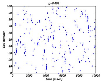 b
b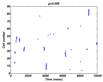
Weakly correlated spontaneous spiking. For sufficiently small, the activity retains the features of spontaneous spiking in the uncoupled population. Fig. 6b shows no significant correlations between the activity of distinct cells in the weakly coupled network. The distributions of the interspike intervals are exponential in both cases (see Fig. 6 (c,d)). There is an important change, however: the rate of firing goes down for increasing values of for small . This is clearly seen from the graphs in Fig. 5. The decreasing firing rate for very weak coupling can also be noted from the interspike interval distributions in Fig. 6c,d: the density in Fig. 6d has a heavier tail. Thus, weak electrical coupling has a pronounced inhibitory (shunting) effect on the network dynamics: it drains the current from a neuron developing a depolarizing potential and redistributes it among the cells connected to it. This effect is stronger for networks with greater number of connections. The three plots shown in Fig. 5a correspond to nearest-neighbor coupling, nearest neighbor coupling, and all-to-all coupling. Note that the slope at zero is steeper for networks with greater degree.
Coherent structures. For increasing values of the system develops clusters, short waves, and robust waves (see Fig. 7). The appearance of these spatio-temporal patterns starts in the middle of the first decreasing portion of the firing rate plot in Fig. 5a and continues through the next (increasing) interval of monotonicity. While patterns in Fig. 7 feature progressively increasing role of coherence in the system’s dynamics, the dynamical mechanisms underlying cluster formation and wave propagation are distinct. Factors A and B below identify two dynamical principles underlying pattern formation in this regime.
Factor A: At the moment when one neuron fires due to large deviations from the rest state, neurons connected to it are more likely to be closer to the threshold and, therefore, are more likely to fire within a short interval of time.
Factor B: When a neuron fires, it supplies neurons connected to it with depolarizing current. If the coupling is sufficiently strong, the gap-junctional current triggers action potentials in these cells and the activity propagates through the network.
Factor A follows from the variational interpretation of the spontaneous dynamics in weakly coupled networks, which we develop in Section 4. It is responsible for the formation of clusters and short waves, like those shown in Fig. 7a. To show numerically that that Factor A (vs. Factor B) is responsible for the formation of clusters, we modified the model (2.6) and (2.7) in the following way. Once a neuron in the network has crossed the threshold, we turn off the current that it sends to the other neurons in the network until it gets back close to the the stable fixed point. We will refer to this model as the modified model (2.6) and (2.7). Numerical results for the modified model in Fig. 8a,b, show that clusters are formed as the result of the subthreshold dynamics, i.e., are due to Factor A. Factor B becomes dominant for stronger coupling. It results in robust waves with constant speed of propagation. The mechanism of the wave propagation is essentially deterministic and is well known from the studies of waves in excitable systems (cf. [24]). However, in the presence of noise, the excitation and termination of waves become random (see Fig. 7(b,c)).
Synchrony. The third interval of monotonicity in the graph of the firing rate vs. the coupling strength is decreasing (see Fig. 5a). It features synchronization, the final dynamical state of the network. In this regime, once one cell crosses the firing threshold the entire network fires in unison. The distinctive feature of this regime is a rapid decrease of the firing rate for increasing (see Fig. 5a). The slowdown of firing in the strong coupling regime was studied in [32] (see also [31, 29, 34]). When the coupling is strong the effect of noise on the network dynamics is diminished by the dissipativity of the coupling operator. The reduced effect of noise results in the decrease of the firing rate. In §5.4, we present analytical estimates characterizing denoising by electrical coupling for the present model.
a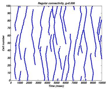 b
b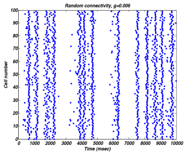
3.2 The role of the network topology
All connected networks of excitable elements (regardless of the connectivity pattern) undergo the three dynamical regimes, which we identified above for weak, intermediate, and strong coupling. The topology becomes important for quantitative description of the activity patterns. In particular, the topology affects the boundaries between different phases. We first discuss the role of topology for the onset of synchronization. The transition to synchrony corresponds to the beginning of the third phase and can be approximately identified with the location of the point of maximum on the firing rate plot (see Fig. 5a,b). The comparison of the plots for and nearest-neighbor coupling schemes shows that the onset of synchrony takes place at a smaller value of for the latter network. This illustrates a general trend: networks with greater number of connections tend to have better synchronization properties. However, the degree is not the only structural property of the graph that affects synchronization. The connectivity pattern is important as well. Fig. 9 shows that a randomly connected degree network synchronizes faster than its symmetric counterpart (cf. Example 2.4). The analysis in §4.4 shows that the point of transition to synchrony can be estimated using the algebraic connectivity of the graph . Specifically, the network is synchronized, if where stands for the coupling strength in the rescaled nondimensional model. The algebraic connectivity is easy to compute numerically. For many graphs with symmetries including those in Examples 2.1-2.3, the algebraic connectivity is known analytically. On the other hand, there are effective asymptotic estimates of the algebraic connectivity available for certain classes of graphs that are important in applications, such as random graphs [15] and expanders [22]. The algebraic connectivities of the graphs in Examples 2.1-2.2 tend to zero as . Therefore, for such networks one needs to increase the strength of coupling significantly to maintain synchrony in networks growing in size. This situation is typical for symmetric or almost symmetric graphs. In contrast, it is known that for the random graph from Example 2.4 the algebraic connectivity is bounded away from zero (with high probability) as [15, 22]. Therefore, one can guarantee synchronization in dynamical networks on such graphs using finite coupling strength when the size of the network grows without bound. This counter-intuitive property is intrinsic to networks on expanders, sparse well connected graphs [22, 36]. For a more detailed discussion of the role of network topology in synchronization, we refer the interested reader to Section in [29].
The discussion in the previous paragraph suggests that connectivity is important in the strong coupling regime. It is interesting that to a large extent the dynamics in the weak coupling regime remains unaffected by the connectivity. For instance, the firing rate plots for the random and symmetric degree- networks (Example 5) shown in Fig. 5b coincide over an interval in near . Furthermore, the plots for the same pair of networks based on the modified model (2.6) and (2.7) are almost identical, regardless the disparate connectivity patterns underlying these networks. The variational analysis in §4.3 shows that, in the weak coupling regime, to leading order the firing rate of the network depends only on the number of connections between cells. The role of the connectivity in shaping network dynamics increases in the strong coupling regime.
4 The variational analysis of spontaneous dynamics
In this section, we analyze dynamical regimes of the coupled system (2.6) and (2.7) under the variation of the coupling strength. In §4.1, we derive an approximate model using the center manifold reduction. In §4.2, we relate the activity patterns of the coupled system to the minima of a certain continuous function on the surface of an cube. The analysis of the minimization problem for weak, strong, and intermediate coupling is used to characterize the dynamics of the coupled system in these regimes.
4.1 The center manifold reduction
In preparation for the analysis of the coupled system (2.6) and (2.7), we approximate it by a simpler system using the center manifold reduction [8, 18]. To this end, we first review the bifurcation structure of the model. Denote the equations governing the deterministic dynamics of a single neuron by
| (4.1) |
where and is a smooth function and is a small parameter, which controls the distance of (4.1) from the saddle-node bifurcation.
Assumption 4.1.
Suppose that at , the unperturbed problem (4.1) has a nonhyperbolic equilibrium at the origin such that has a single zero eigenvalue and the rest of the spectrum lies to the left of the imaginary axis. Suppose further that at there is a homoclinic orbit to entering the origin along the center manifold.

Then under appropriate nondegeneracy and transversality conditions on the local saddle-node bifurcation at , for near zero the homoclinic orbit is transformed into either a unique asymptotically stable periodic orbit or to a closed invariant curve having two equilibria: a node and a saddle [8] (Fig. 10). Without loss of generality, we assume that the latter case is realized for small positive , and the periodic orbit exists for negative . Let be a sufficiently small fixed number, i.e., (4.1) is in the excitable regime (Fig. 10). For simplicity, we assume that the stable node near the origin is the only attractor of (4.1).
We are now in a position to formulate our assumptions on the coupled system. Consider local systems (4.1) that are placed at the nodes of the connected graph and coupled electrically:
| (4.2) |
where , is an identity matrix, , and is the Laplacian of . Matrix defines the linear combination of the local variables engaged in coupling. In the the neuronal network model above, . Parameters and control the coupling strength and the noise intensity respectively. is a Gaussian white noise process in . The local systems are taken to be identical for simplicity. The analysis can be extended to cover nonhomogeneous networks.
We next turn to the center manifold reduction of (4.2). Consider (4.2 (the zero subscript refers to ) for . By our assumptions on the local system (4.1), has a kernel. Denote
| (4.3) |
By the center manifold theorem, there is a neighborhood of the origin in the phase space of (4.2), , and such that for and , in , there exists an attracting locally invariant dimensional slow manifold . The trajectories that remain in for sufficiently long time can be approximated by those lying in . Thus, the dynamics of (4.2 can be reduced to , whose dimension is times smaller than that of the phase space of (4.2. The center manifold reduction is standard. Its justification relies on the Lyapunov-Schmidt method and Taylor expansions (cf. [8]). Formally, the reduced system is obtained by projecting (4.2 onto the center subspace of (4.2 for (see [25]):
| (4.4) |
where provided that the following nondegeneracy conditions hold
| (4.5) | |||||
| (4.6) | |||||
| (4.7) |
Conditions (4.5) and (4.6) are the nondegeneracy and transversality conditions of the saddle-node bifurcation in the local system (4.1). Condition (4.7) guarantees that the projection of the coupling onto the center subspace is not trivial. All conditions are open. Without loss of generality, assume that nonzero coefficients are positive.
Next, we include the random perturbation in the reduced model. Note that near the saddle-node bifurcation (), the vector field of (4.2 is much stronger in the directions transverse to than in the tangential directions. The results of the geometric theory of randomly perturbed fast-slow systems imply that the trajectories of (4.2) with small positive that start close to the node of (4.2 remain in a small neighborhood of on finite intervals of time with overwhelming probability (see [3] for specific estimates). To obtain the leading order approximation of the stochastic system (4.2) near the slow manifold, we project the random perturbation onto the center subspace of (4.2 for and add the resultant term to the reduced equation (4.4):
| (4.8) |
We replace by identically distributed , where is a white noise process in and . Here, stands for the Euclidean norm of . After rescaling the resultant equation and ignoring the higher order terms, we arrive at the following reduced model
| (4.9) |
where stands for a standard Brownian motion in and Here, with a slight abuse of notation, we continue to use to denote the small parameter in the rescaled system. In the remainder of this paper, we analyze the reduced model (4.9).
4.2 The exit problem
In this subsection, the problem of identifying most likely dynamical patterns generated by (4.2) is reduced to a minimization problem for a smooth function on the surface of the unit cube.
Consider the initial value problem for (4.9)
| (4.10) |
where
| (4.11) |
and
| (4.12) |
where auxiliary parameter will be specified later. Let
| (4.13) |
denote a subset of the boundary of D, . If , then at least one of the neurons in the network is at the firing threshold. It will be shown below that the trajectories of (4.10) exit from through with probability as , provided is sufficiently large.111Positive parameter in the definition of (cf. (4.12)) is used to exclude the possibility of exit from through . Therefore, the statistics of the first exit time
| (4.14) |
and the distribution of the location of the points of exit characterize the statistics of the interspike intervals and the most probable firing patterns of (2.1) and (2.2), respectively. The Freidlin-Wentzell theory of large deviations [14] yields the asymptotics of and for small .
To apply the large deviation estimates to the problem at hand, we rewrite (4.10) as a randomly perturbed gradient system
| (4.15) |
where
| (4.16) |
where stands for the inner product in . The additive constant in the definition of the potential function is used to normalize the value of the potential at the local minimum .
The following theorem summarizes the implications of the large deviation theory for (4.15).
Theorem 4.2.
Let denote the points of minima of on
and . Then for any and ,
| (4.17) | |||||
| (4.18) | |||||
| (4.19) |
where stands for the distance in .
The statements A)-C) can be shown by adopting the proofs of Theorems 2.1, 3.1, and 4.1 of Chapter 4 of [14] to the case of the action functional with multiple minima.
4.3 The weak coupling regime
In this subsection, we study the minima of on for small . First, we locate the points of minima of the for (cf. Lemma 4.3). Then, using the Implicit Function Theorem, we continue them for small (cf. Theorem 4.4).
Lemma 4.3.
Let in the definition of (4.12) be fixed. The minimum of on is achieved at points
| (4.21) |
The minimal value of on is
| (4.22) |
Proof. Denote
and .
Consider the restriction of on
| (4.23) |
where . The gradient of is equal to
The definition of (4.11) implies that restricted to has a unique critical point at and On the other hand, on the boundary of , , the minimum of satisfies
for any in (4.12).
Likewise, as follows from the definitions of (4.16) and
(4.12), for ,
for any choice of in (4.12). Thus,
minimizes over . The lemma is proved by
repeating the above argument for the remaining faces
,
.
Theorem 4.4.
Suppose in (4.12) is sufficiently large. There exists such that for on each face , achieves minimum
where is a smooth function such that
| (4.24) |
and is the th column of the graph Laplacian after deleting the th entry. The equations in (4.24) are written using the following local coordinates for
Moreover, the minimal value of on is given by
| (4.25) |
Consequently,
| (4.26) |
Proof. Let denote the restriction of on :
| (4.27) |
where
Next, we compute the gradient of :
| (4.28) |
where . Further,
| (4.38) |
where stands for the matrix obtained from by deleting the th row and th column. By plugging (4.38) in (4.28), we have
| (4.39) |
The equation for the critical points has the following form
| (4.40) |
Note that
| (4.41) |
Above we used the relation
| (4.42) |
which follows from the fact that the rows of sum to zero.
By the Implicit Function Theorem, for small , the unique solution of (4.40) is given by the smooth function that satisfies
| (4.43) |
By taking into account,
from (4.43) we have
| (4.44) |
This shows (4.24). To show (4.25), we use the Taylor expansion of :
| (4.45) | |||||
By choosing in (4.12) large enough one can ensure that
for
remains smaller than the values of on the boundary .
To complete the proof, one only needs to apply the same argument
to all other faces of , and note that on ,
the values of , can be made arbitrarily large by choosing
sufficiently large in (4.12).
Remark 4.5.
The second equation in (4.24) shows that the minima of the potential function lying on the faces corresponding to connected cells move towards the common boundaries of these faces, under the variation of .
4.4 The strong coupling regime
For small , the minima of are located near the minima of the potential function (cf. (4.16)). In this subsection, we show that for larger , the minima of are strongly influenced by the quadratic term , which corresponds to the coupling operator in the differential equation model (4.10). To study the minimization problem for , we rewrite as follows:
| (4.46) |
Thus, the problem of minimizing for becomes the minimization problem for
| (4.47) |
Lemma 4.6.
attains the global minimum on at :
| (4.48) |
Proof. is nonnegative, moreover,
Finally, .
Theorem 4.7.
Let denote the smallest eigenvalue of matrix , obtained from by deleting the th row and the th column. Then for , achieves its minimal value on at :
| (4.49) |
provided in the definition of (cf. (4.12)) is sufficiently large.
Remark 4.8.
By the interlacing eigenvalues theorem (cf. Theorem 4.3.8, [21]), (Note that is not a graph Laplacian.) Furthermore, , because is connected (cf. Theorem 6.3, [6]). With these observations, Theorem 4.7 yields an estimate for the onset of synchrony in terms of the eigenvalues of :
| (4.50) |
Note that (4.50) yields smaller lower bounds for the onset of synchrony for graphs with larger algebraic connectivity. In particular, for the families of expanders (cf. Example 2.5), it provides bounds on the coupling strength guaranteeing synchronization that are uniform in .
For the proof of Theorem 4.7, we need the following auxiliary lemma.
Lemma 4.9.
For there exists such that
| (4.51) |
where is defined by
| (4.52) |
Proof. Since , for some . Without loss of generality, let . Then
and
where the quadratic function . Differentiating yields:
Therefore,
Proof. (Theorem 4.7) Let . By Lemma 4.9, for some and defined in (4.52), we have
| (4.53) |
We will use the following observations:
- (a)
-
is a positive definite matrix, and, therefore,
- (b)
-
For ,
- (c)
-
Using (a) and (b), from (4.53), we have
provided .
This shows that minimizes on for
.
On the other hand, on , can be made arbitrarily large
for any provided in (4.12) is sufficiently large.
4.5 Intermediate coupling strength: formation of clusters
In this subsection, we develop a geometric interpretation of the spontaneous dynamics of (2.6) and (2.7). After introducing certain auxiliary notation, we discuss how the spatial location of the minima of on the surface of the cube encodes the most likely activity patterns of (2.6) and (2.7). Then we proceed to derive a lower bound on the coupling strength necessary for the development of coherent structures.
Let and define a -dimensional face of as
| (4.54) |
The union of all -dimensional faces is denoted by
| (4.55) |
Suppose is a point of minimum of on . If , , then with high probability the network discharges in clusters. The analysis in §4.3 shows that for small there is practically no correlation between the activity of distinct neurons. On the other hand, when the coupling is strong, all cells fire in unison (cf. §4.4). Lemma 4.10 provides a lower bound on the coupling strength needed for the formation of clusters.
Lemma 4.10.
Let be a point of global minimum of on . If for some then
| (4.56) |
Proof. Suppose . Without loss of generality, we assume that
Denote and . Thus,
| (4.57) | |||||
| (4.58) |
where is a matrix obtained from by deleting the first and the second rows and columns. The Laplacian of can be represented as
where the adjacency matrix is nonnegative (cf. (2.11)). Therefore, for nonnegative ,
| (4.59) |
Further, for any ,
| (4.60) |
provided . The combination of (4.57)-(4.60) yields
| (4.61) |
for . By (4.61),
provided
| (4.62) |
The statement of the lemma follows from the observation above by noting
that in (4.62) is arbitrary.
5 An alternative view on synchrony
The variational analysis of the previous section shows that when the coupling is strong (), the neurons in the network fire together (cf. Theorem 4.7). In this section, we use a complementary approach to studying synchrony in the coupled system. We show that strong coupling brings about the separation of the timescales in the system’s dynamics, which defines two principal modes in the strong coupling regime: the fast synchronization and slow large-deviation type escape from the potential well. The analysis of the fast subsystem elucidates the stability of the synchronization subspace. In particular, it reveals the contribution of the network topology to the robustness of synchrony. The analysis of the slow subsystem yields the asymptotic rate of the network activity in the strong coupling regime (cf. Theorem 4.7).
5.1 The slow-fast decomposition
Our first goal is to show that when coupling is strong the dynamics of the coupled system (4.10) has two disparate timescales. To this end, we introduce the following coordinate transformation
where
| (5.1) |
and is the coboundary matrix corresponding to the spanning tree of (see (2.9)).
Lemma 5.1.
Proof. Fix . For each there exists a unique path connecting nodes and and belonging to
| (5.4) |
Thus,
| (5.5) |
where . By summing equations (5.5), adding the identity to the resultant equation, and dividing the result by , we obtain
| (5.6) |
The first inequality in (5.3) follows from the formula for in (5.6) and . To show the second identity in (5.3), add up equations (5.6) for and use the definition of :
Lemma 5.2.
Suppose is a connected graph and is its Laplacian. There exists a unique such that
| (5.7) |
where is the coboundary matrix of the , a spanning tree of . The spectrum of consists of all nonzero eigenvalues of
| (5.8) |
Proof. Since is connected and is a spanning tree of ,
| (5.9) |
The existence and uniqueness of the solution of the matrix equation (5.7), ,
is shown in Lemma 2.3 of [29]. Equation (5.8)
follows from Lemma 2.5 of [29].
We are now in a position to rewrite (4.10) in terms of .
Lemma 5.3.
The following system of stochastic differential equations is equivalent in law to (4.10):
| (5.10) | |||||
| (5.11) |
where
| (5.12) |
Throughout this section, and denote the white noise processes in and respectively.
5.2 Fast dynamics: synchronization
For , the system of equations (5.10) and (5.11) has two disparate timescales. The stable fixed point of the fast subsystem (5.10) corresponds to the synchronous state of (4.10)
In this section, we analyze the stability of the steady state of the fast subsystem. Specifically, we identify the network properties that determine the rate of convergence of the trajectories of the fast subsystem to the steady state and its degree of stability to random perturbations. These results elucidate the contribution of the network topology to the synchronization properties of the coupled system (4.10).
By switching to the fast time (5.10) and (5.11), we have
| (5.14) | |||||
| (5.15) |
where
| (5.16) |
The leading order approximation of the fast equation (5.14) does not depend on the slow variable :
| (5.17) |
The solution of (5.17) with deterministic initial condition is a Gaussian random process. The mean vector and the covariance matrix functions
| (5.18) |
satisfy linear equations
| (5.19) |
Recall that is a positive definite matrix, whose smallest eigenvalue is equal to the algebraic connectivity of , (see Lemma 5.2). By integrating the first equation in (5.19), we find that
| (5.20) |
for some . Thus, the trajectories of the fast subsystem converge in mean to the stable fixed point , which corresponds to the synchronization subspace of (4.10). Moreover, the rate of convergence is set by the algebraic connectivity .
Further,
| (5.21) |
measures the spread of the trajectories around the synchronization subspace. By integrating the second equation in (5.19), we have
| (5.22) | |||||
where
| (5.23) |
Parameter quantifies the mean square stability of the synchronization subspace. In §5.4, we show that depends on the properties of the cycle subspace of .
For small , a typical trajectory of (5.17) converges to a small neighborhood of the stable equilibrium at the origin. However, eventually it leaves the neighborhood of the origin under persistent random perturbations. Next, we estimate the time that the trajectory of the fast subsystem spends near the origin.
Let and . By we denote the solution of (5.17) satisfying initial condition . Define the first exit time of the trajectory of (5.17) from :
| (5.24) |
Using the large deviation estimates (cf. [14]), we have
| (5.25) |
where
| (5.26) |
is the minimum of the positive definite quadratic form on the boundary of .
By combining (5.25) and (5.26) we obtain the logarithmic asymptotics of the first exit time from
| (5.27) |
For small (i.e., for large ), (5.27) applies to the fast equation (5.14). Switching back to the original time, we rewrite the estimate for the first exit time for the fast equation (5.10):
| (5.28) |
Finally, choosing for an arbitrary fixed , we have
| (5.29) |
5.3 The slow dynamics: escape from the potential well
We recap the results of the analysis of the fast subsystem. The trajectories of the fast subsystem (5.10) enter an neighborhood of the stable equilibrium (corresponding to the synchronization subspace of the full system) in time and remain there with overwhelming probability over time intervals . During this time, the dynamics is driven by the slow equation (5.11), which we analyze next.
While the trajectory of the fast subsystem stays in the neighborhood of the equilibrium, the quadratic term in (5.11) is small. Thus, the leading order approximation of the slow equation is independent of on time intervals
| (5.30) |
Equation (5.30) has a stable fixed point at the origin, where the potential function attains its minimum value (see (4.16)). The escape of the trajectories of (5.30) from the potential well, defined by corresponds to spontaneous synchronized discharge of the coupled subsystem. Suppose and define
| (5.31) |
By the large deviation theory, we have
| (5.32) |
Equation (5.32) provides the estimate for the frequency of spontaneous activity in the strong coupling regime. Note that (5.32) is consistent with the estimate in Theorem 4.7 derived using the variational argument. Therefore, the analysis in this section yields the dynamical interpretation for the minimization problem for (4.20) in the strong coupling regime.
We summarize the results of the slow-fast analysis. In the strong coupling regime, the dynamics splits into two modes: fast synchronization and slow synchronized fluctuations leading to large deviation type discharges of the entire network. By analyzing the fast subsystem, we obtained estimates of stability of the synchronization subspace. The analysis of the slow subsystem yields the asymptotic estimate of the firing rate in the strong coupling regime.
5.4 The network topology and synchronization
The stability analysis in §5.2 provides interesting insights into what structural properties of the network are important for synchronization. In this subsection, we discuss the implications of the stability analysis in more detail.
First, we rewrite (5.20) and (5.22), using the original time
| (5.33) | |||||
| (5.34) |
where . Equation (5.33) shows that the rate of convergence to the synchronous state depends on the coupling strength, , and the algebraic connectivity of the network, . The convergence is faster for stronger coupling and larger . This, in particular, implies that the rate of convergence to synchrony in networks on spectral expanders (cf. Example 2.5) remains as the size of the network grows without bound. In particular, the families of the random graphs (cf. Example 2.4) have this property. In contrast, for many networks with symmetries (cf. Example 2.2) the algebraic connectivity as , and, therefore, by (5.33), synchronization requires longer time, if the size of the network grows. For a more detailed discussion of the synchronization properties of the networks on expanders, we refer the interested reader to [29].
Next, we turn to Equation (5.34), which characterizes the dispersion of the trajectories around the synchronization subspace. may be viewed as a measure of robustness of synchrony to noise or, more generally, to constantly acting perturbations. By (5.34), the synchrony is more robust for stronger coupling, because the asymptotic value of as . The contribution of the network topology to the mean-square stability of the synchronous state is reflected in . Trajectories of the networks with smaller are more tightly localized around the synchronization subspace.
To explain the graph-theoretic interpretation of , we review the structure of the cycle subspace of . Recall that the edge set of the spanning tree consists of the first edges (see (2.9)):
If is not a tree, then
where is the corank of . To each edge , there corresponds a unique cycle of length , such that it consists of and the edges from . The following lemma, relates the value of to the properties of the cycles .
Lemma 5.4.
[29] Let be a connected graph.
- A
-
If is a tree then
(5.35) - B
-
Otherwise, let be a spanning tree of a and be the corresponding independent cycles.
- B.1
-
Denote
Then
(5.36) - B.2
-
If then
(5.37) where
- B.3
-
If are disjoint. Then
(5.38) In particular,
and
The asymptotic estimate of the mean square stability of the synchronization subspace in (5.34) combined with the estimates of in Lemma 5.4 show how the structure of the cycle subspace of translates into the stability of the synchronous state. In [29], one can also find an estimate of the asymptotic stability of the synchronization subspace in terms of the effective resistance of the graph . These results show how the structural properties of the network shape synchronization properties of the coupled system.
a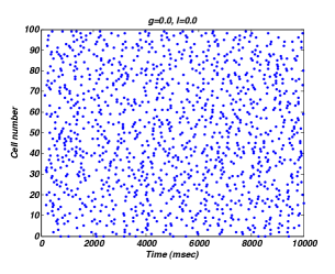 b
b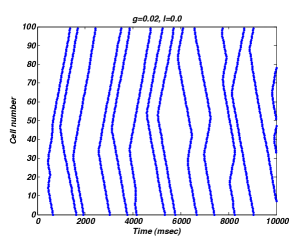
c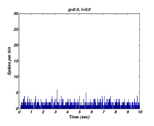 d
d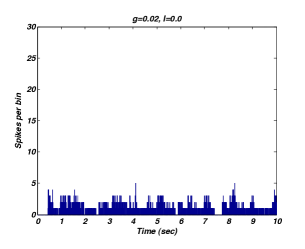
e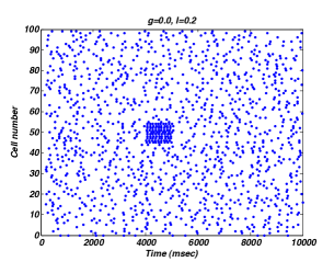 f
f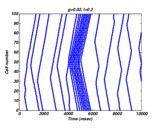
g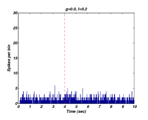 h
h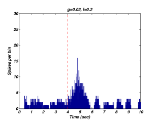
6 Discussion
In this paper, we presented a variational method, which reduces the problem of pattern-formation in electrically coupled networks of neurons to the minimization problem for the potential function on the surface of a unit cube, . The variational problem provides geometric interpretation for the spontaneous dynamics generated by the network. Specifically, the location of the points of minima of the constrained potential function corresponds to the most likely patterns of network activity.
The variational formulation has several important implications for the analysis of the dynamical problem. First, the minimization problem has an intrinsic bifurcation structure. By a bifurcation of the problem (4.20), it is natural to call the value of the parameter corresponding to the structural changes in the singularity set of . For example, the number of the minima of can change due to collisions of the singularities with each other or with the boundaries of the faces of a given co-dimension (a border collision bifurcation). In either case, the qualitative change in the configuration of the points of minima of signals the transformation of the attractor of the randomly perturbed system (4.10). The study of the constrained minimization problem (4.20) identified three main regimes in the network dynamics for weak, intermediate, and strong coupling. These results hold for any connected network. We expect that under certain assumptions on the network topology (e.g., in the presence of symmetries, or alternatively in networks with random connections), a more detailed description of the bifurcation events preceding complete synchronization should be possible.
The analysis of the variational problem has also helped to obtain quantitative estimates for the network dynamics. For both weak and strong coupling, we derived the asymptotic formulae for the dependence of the firing rate as a function of the coupling strength (see (4.26) and (4.49)). Surprisingly, in each of these cases, the firing rate does not depend on the structure of the graph of the network beyond its degree and order. In particular, the network of equal degree with connectivity patterns as different as symmetric and random exhibit the same activity rate (see Fig. 5c).
The geometric interpretation of the spontaneous dynamics yields a novel mechanism of the formation of clusters. It shows that the network fires in clusters, whenever has a minimum on a co-dimension face of . In particular, the network becomes completely synchronized, when the minimum of reaches . This observation allows one to estimate the onset of synchronization (cf. Theorem 4.7) and cluster formation (cf. Lemma 4.10). Furthermore, we show that in the strong coupling regime, the network dynamics has two disparate timescales: fast synchronization is followed by an ultra-slow escape from the potential well. The analysis of the slow-fast system yields estimates of stability of the synchronous state in terms of the coupling strength and structural properties of the network. In particular, it shows the contribution of the network topology to the synchronization properties of the network.
We end this paper with a few concluding remarks about the implications of this work for the LC network. The analysis of the conductance-based model of the LC network in this paper agrees with the study of the integrate-and-fire neuron network in [38] and confirms that the assumptions of spontaneously active LC neurons coupled electrically with a variable coupling strength are consistent with the experimental observations of the LC network. Following the observations in [38] that stronger coupling slows down network activity, we have studied how the firing rate depends on the coupling strength. We show that strong coupling results in synchronization and significantly decreases the firing rate (see also [32, 34]). Surprisingly, we found that the rate can be effectively controlled by the strength of interactions already for very weak coupling. We show that the dependence of the firing rate on the strength of coupling is nonmonotone. This has an important implication for the interpretation of the experimental data. Because two distinct firing patterns can have similar firing rates, the firing rate alone does not determine the response of the network to external stimulation. This situation is illustrated in Fig. 11. We choose parameters such that two networks, the spontaneously active (Fig. 11a) and the nearly synchronous one (Fig. 11b), exhibit about the same activity rates (see Fig. 11c,d). However, because the activity patterns generated by these networks are different, so are their responses to stimulation (Fig. 11e,f). The network in the spontaneous firing regime produces a barely noticeable response (Fig. 11g), whereas the response of the synchronized network is pronounced (Fig. 11h). Network responses similar to these were observed experimentally and are associated with the good (Fig. 11h) and poor (Fig. 11g) cognitive performance [38]. Our analysis suggests that the state of the network (i.e., the spatio-temporal dynamics) rather than the firing rate, determines the response of the LC network to afferent stimulation.
The main hypotheses used in our analysis are that the local dynamical systems satisfy Assumption 4.1 and interact through electrical coupling. The latter means that the coupling is realized through one of the local variables, interpreted as voltage, and is subject to the two Kirchhoff’s laws for electrical circuits. In this form our assumptions cover many biological, physical, and technological problems, including power grids, sensor and communication networks, and consensus protocols for coordination of autonomous agents (see [29] and references therein). Therefore, the results of this work elucidate the principles of pattern formation in an important class of problems.
Acknowledgments. This work was partly supported by the NSF Award DMS 1109367 (to GM).
Appendix. The parameter values used in the biophysical model (2.1) and (2.2)
To emphasize that the results of this study do not rely on any specific features of the LC neuron model, in our numerical experiments we used the Morris-Lecar model, a common Type I biophysical model of an excitable cell [35]. This model is based on the Hodgkin-Huxley paradigm. The function on the right hand side of the voltage equation (2.1), , models the combined effect of the calcium and sodium currents, , the potassium current, , and a small leak current, ,
Constants , , and stand for the reversal potentials and , , and denote the maximal conductances of the corresponding ionic currents. The activation of the calcium and potassium channels are modeled using the steady-state functions
and the voltage-dependent time constant
The parameter values are summarized the following table.
Table
| 120 | 8 | -84 | 18 | 4 | 0.067 | ||||||
| 2 | -60 | 20 | -1.2 | 12 | 17.4 |
References
- [1] G. Aston-Jones and J.D. Cohen, An integrative theory of Locus Coeruleus-Norepinephrine function: adaptive gain and optimal performance, Annu. Rev. Neurosci., 28:403-50, 2005.
- [2] V. Alvarez, C. Chow, E.J. Van Bockstaele, and J.T. Williams, Frequency-dependent synchrony in locus coeruleus: role of electronic coupling, Proc. Nat. Acad. Sci. USA, , 4032–4036, 2002.
- [3] N. Berglund and B. Gentz, Noise-Induced Phenomena in Slow-Fast Dynamical Systems: A Sample-Paths Approach, Springer, 2006.
- [4] Berridge, C.W. and Waterhouse, B.D., The locus coeruleus-noradrenergic system: modulation of behavioral state and state-dependent cognitive processes, Brain Research Reviews, 42, 33-84, 2003.
- [5] Brown, Eric and Moehlis, Jeff and Holmes, Philip and Clayton, Ed and Rajkowski, Janusz and Aston-Jones, Gary, The influence of spike rate and stimulus duration on noradrenergic neurons, Journal of Comp. Neuroscience,17, 13-29, 2004.
- [6] N. Biggs, Algebraic Graph Theory, second ed., Cambridge University Press, 1993.
- [7] Bela Bollobas, Modern graph theory, Graduate Texts in Mathematics, vol. 184, Springer, New York, 1998.
- [8] S.-N. Chow and J.K. Hale, Methods Of Bifurcation Theory, Springer-Verlag New York Inc, New York, 1982.
- [9] F.R.K. Chung, Spectral Graph Theory, CBMS Regional Conference Series in Mathematics, No. 92, 1997.
- [10] B.W. Connors and M.A. Long, Electrical synapses in the mammalian brain, Annu. Rev. Neurosci., 27:393–418, 2004.
- [11] S. Coombes, Neuronal networks with gap junctions: A study of piece-wise linear planar neuron models, SIAM Journal on Applied Dynamical Systems, , 1101–1129, 2008.
- [12] Martin V. Day, On the exponential exit law in the small parameter exit problem, Stochastics, , 297–323, 1983.
- [13] M.I. Freidlin, On stable oscillations and equilibriums induced by small noise, J. of Stat. Phys., (1-2), 283–300, 2001.
- [14] M.I. Freidlin and A.D. Wentzell, Random perturbations of dynamical systems, 2nd ed., Springer, New York, 1998.
- [15] J. Friedman, A Proof of Alon’s Second Eigenvalue Conjecture and Related Problems, Memoirs of the American Mathematical Society, vol. 195, 2008.
- [16] M. Fiedler, Algebraic connectivity of graphs. Czech. Math. J. 23(98), 1973.
- [17] J. Jost, Dynamical networks, in J. Feng, J. Jost, and M. Qian, (Eds.) Networks: From Biology to Theory, Springer, 2007
- [18] J. Guckenheimer and P. Holmes, Nonlinear Oscillations, Dynamical Systems, and Bifurcations of Vector Fields, Springer, 1983.
- [19] Juan Gao and Philip Holmes, On the dynamics of electrically-coupled neurons with inhibitory synapses, J. Comput. Neurosci., 22:39–61, 2007.
- [20] J.K Hale, Ordinary Differential Equations, Krieger, 2nd edition, 1980.
- [21] R.A. Horn and C.R. Johnson, Matrix Analysis, Cambridge University Press, 1999.
- [22] S. Hoory, N. Linial, and A. Wigderson, Expander graphs and their applications, Bulletin of the American Mathematical Society, vol. 43, no. 4, pp 439–561, 2006.
- [23] I. Karatzas and S.E. Shreve, Brownian Motion and Stochastic Calculus, 2nd ed., Springer, New York, 1991.
- [24] James P. Keener, Propagation and its failure in coupled systems of discrete excitable cells, SIAM Journal on Applied Mathematics, v.47 n.3, p.556-572, 1987.
- [25] Yuri A. Kuznetsov, Elements of applied bifurcation theory, Springer, 1998.
- [26] T. Lewis and J. Rinzel, Dynamics of spiking neurons connected by both inhibitory and electrical coupling, J. Comp. Neurosci., 14:283–309, 2003.
- [27] A. Lubotzky, R. Phillips, and P. Sarnak, Ramanujan graphs, Combinatorica, , 161–278, 1988.
- [28] G. Margulis, Explicit group-theoretic constructions of combinatorial schemes and their applications in the construction of expanders and concentrators. (Russian) Problemy Peredachi Informatsii 24 (1988), no. 1, 51–60; (English translation in Problems Inform. Transmission 24 (1988), no. 1, 39–46).
- [29] G.S. Medvedev, Stochastic stability of continuous time consensus protocols, submitted, arXiv preprint: 1007.1234.
- [30] G.S. Medvedev, Synchronization of coupled limit cycles, J. Nonlin. Sci., , 441–464, 2011.
- [31] G.S. Medvedev, Synchronization of coupled stochastic limit cycle oscillators, Physics Letters A (374), 1712–1720, 2010.
- [32] G.S. Medvedev, Electrical coupling promotes fidelity of responses in the networks of model neurons, Neural Computation, (11), 3057–3078, 2009.
- [33] G.S. Medvedev and N. Kopell, Synchronization and transient dynamics in the chains of electrically coupled FitzHugh-Nagumo oscillators, SIAM J. of Appl. Math., , 1762–1801, 2001.
- [34] G.S. Medvedev and S. Zhuravytska, Shaping bursting by electrical coupling and noise, submitted, arXiv preprint: 1111.0642.
- [35] J. Rinzel and G.B. Ermentrout, Analysis of neural excitability and oscillations, in C. Koch and I. Segev, eds Methods in Neuronal Modeling, MIT Press, Cambridge, MA, 1989.
- [36] P. Sarnak, What is an expander?, Notices of the American Mathematical Society, 51, 762–763, 2004.
- [37] S.J. Sara, The locus coeruleus and noradrenergic modulation of cognition, Nat. Rev. Neurosci., 10, 211-223, 2009.
- [38] M. Usher, J.D. Cohen, D. Servan-Schreiber, J. Rajkowski and G. Aston-Jones, The role of locus coeruleus in the regulation of cognitive performance, Science, (1999), pp. 549–554.