$\ell_{0}$ Minimization for Wavelet Frame Based Image Restoration

Abstract.

The theory of (tight) wavelet frames has been extensively studied in the past twenty years and they are currently widely used for image restoration and other image processing and analysis problems. The success of wavelet frame based models, including balanced approach [18, 7] and analysis based approach [11, 31, 50], is due to their capability of sparsely approximating piecewise smooth functions like images. Motivated by the balanced approach and analysis based approach, we shall propose a wavelet frame based $\ell_{0}$ minimization model, where the $\ell_{0}$ “norm” of the frame coefficients is penalized. We adapt the penalty decomposition (PD) method of [40] to solve the proposed optimization problem. Some convergence analysis of the adapted PD method will also be provided. Numerical results showed that the proposed model solved by the PD method can generate images with better quality than those obtained by either analysis based approach or balanced approach in terms of restoring sharp features as well as maintaining smoothness of the recovered images.

1. Introduction

Mathematics has been playing an important role in the modern developments of image processing and analysis. Image restoration, including image denoising, deblurring, inpainting, tomography, etc., is one of the most important areas in image processing and analysis. Its major purpose is to enhance the quality of a given image that is corrupted in various ways during the process of imaging, acquisition and communication; and enable us to see crucial but subtle objects residing in the image. Therefore, image restoration is an important step to take towards accurate interpretations of the physical world and making optimal decisions.

1.1. Image Restoration

Image restoration is often formulated as a linear inverse problem. For the simplicity of the notations, we denote the images as vectors in ${{\mathbb{R}}}^{n}$ with $n$ equals to the total number of pixels. A typical image restoration problem is formulated as

(1.1) $$f=Au+\eta,$$

where $f\in{{\mathbb{R}}}^{d}$ is the observed image (or measurements), $\eta$ denotes white Gaussian noise with variance $\sigma^{2}$, and $A\in{{\mathbb{R}}}^{d\times n}$ is some linear operator. The objective is to find the unknown true image $u\in{{\mathbb{R}}}^{n}$ from the observed image $f$. Typically, the linear operator in (1.1) is a convolution operator for image deconvolution problems, a projection operator for image inpainting and partial Radon transform for computed tomography.

To solve $u$ from (1.1), one of the most natural choices is the following least square problem

$$\min_{u\in{{\mathbb{R}}}^{n}}\|Au-f\|_{2}^{2},$$

where $\|\cdot\|_{2}$ denotes the $\ell_{2}$-norm. This is, however, not a good idea in general. Taking image deconvolution problem as an example, since the matrix $A$ is ill-conditioned, the noise $\eta$ possessed by $f$ will be amplified after solving the above least squares problem. Therefore, in order to suppress the effect of noise and also preserve key features of the image, e.g., edges, various regularization based optimization models were proposed in the literature. Among all regularization based models for image restoration, variational methods and wavelet frames based approaches are widely adopted and have been proven successful.

The trend of variational methods and partial differential equation (PDE) based image processing started with the refined Rudin-Osher-Fatemi (ROF) model [45] which penalizes the total variation (TV) of $u$. Many of the current PDE based methods for image denoising and decomposition utilize TV regularization for its beneficial edge preserving property (see e.g., [41, 46, 42]). The ROF model is especially effective on restoring images that are piecewise constant, e.g., binary images. Other types of variational models were also proposed after the ROF model. We refer the interested readers to [36, 17, 41, 42, 22, 2, 23, 53] and the references therein for more details.

Wavelet frame based approaches are relatively new and came from a different path. The basic idea for wavelet frame based approaches is that images can be sparsely approximated by properly designed wavelet frames, and hence, the regularization used for wavelet frame based models is the $\ell_{1}$-norm of frame coefficients. Although wavelet frame based approaches take similar forms as variational methods, they were generally considered as different approaches than variational methods because, among many other reasons, wavelet frame based approaches is defined for discrete data, while variational methods assume all variables are functions. Some studies in the literature (see for example [51]) indicated that there was a relation between Haar wavelet and total variation. However, it was not clear if there exists a general relation between wavelet frames and variational models (with general differential operators) in the context of image restorations. In a recent paper [9], the authors established a rigorous connection between one of the wavelet frame based approaches, namely the analysis based approach, and variational models. It was shown in [9] that the analysis based approach can be regarded as a finite difference approximation of a certain type of general variational model, and such approximation will be exact when image resolution goes to infinity. Furthermore, through Gamma-convergence, the authors showed that the solutions of the analysis based approach also approximate the solutions of the corresponding variational model. Such connections not only grant geometric interpretation to wavelet frame based approaches, but also lead to even wider applications of them, e.g., image segmentation [27] and 3D surface reconstruction from unorganized point sets [29]. On the other hand, the discretization provided by wavelet frames was shown, in e.g., [18, 20, 10, 11, 9, 28], to be superior than the standard discretizations for some of the variational models, due to the multiresolution structure and redundancy of wavelet frames which enable wavelet frame based models to adaptively choose a proper differential operators in different regions of a given image according to the order of the singularity of the underlying solutions. For these reasons, as well as the fact that digital images are always discrete, we use wavelet frames as the tool for image restoration in this paper.

1.2. Wavelet Frame Based Approaches

We now briefly introduce the concept of tight frames and tight wavelet frame, and then recall some of the frame based image restoration models. Interesting readers should consult [44, 24, 25] for theories of frames and wavelet frames, [47] for a short survey on theory and applications of frames, and [28] for a more detailed survey.

A countable set $X\subset L_{2}(\mathbb{R})$ is called a tight frame of $L_{2}(\mathbb{R})$ if

$$f=\sum_{h\in X}\langle f,h\rangle h\quad\forall f\in L_{2}(\mathbb{R}),$$

where $\langle\cdot,\cdot\rangle$ is the inner product of $L_{2}(\mathbb{R})$. The tight frame $X$ is called a tight wavelet frame if the elements of $X$ are generated by dilations and translations of finitely many functions called framelets. The construction of framelets can be obtained by the unitary extension principle (UEP) of [44]. In our implementations, we will mainly use the piecewise linear B-spline framelets constructed by [44]. Given a 1-dimensional framelet system for $L_{2}(\mathbb{R})$, the $s$-dimensional tight wavelet frame system for $L_{2}(\mathbb{R}^{s})$ can be easily constructed by using tensor products of 1-dimensional framelets (see e.g., [24, 28]).

In the discrete setting, we will use $W\in{{\mathbb{R}}}^{m\times n}$ with $m\geq n$ to denote fast tensor product framelet decomposition and use $W^{\top}$ to denote the fast reconstruction. Then by the unitary extension principle [44], we have $W^{\top}W=I$, i.e., $u=W^{\top}Wu$ for any image $u$. We will further denote an $L$-level framelet decomposition of $u$ as

$$Wu=\left(\ldots,{W}_{l,j}u,\ldots\right)^{\top}\quad\mbox{for }0\leq l\leq L-1,j\in\mathcal{I},$$

where $\mathcal{I}$ denotes the index set of all framelet bands and $W_{l,j}u\in{{\mathbb{R}}}^{n}$. Under such notation, we have $m=L\times|\mathcal{I}|\times n$. We will also use $\alpha\in{{\mathbb{R}}}^{m}$ to denote the frame coefficients, i.e., $\alpha=Wu$, where

$$\alpha=\left(\ldots,\alpha_{l,j},\ldots\right)^{\top},\quad\mbox{with}\ \alpha_{l,j}=W_{l,j}u.$$

More details on discrete algorithms of framelet transforms can be found in [28].

Since tight wavelet frame systems are redundant systems (i.e., $m>n$), the representation of $u$ in the frame domain is not unique. Therefore, there are mainly three formulations utilizing the sparseness of the frame coefficients, namely, analysis based approach, synthesis based approach, and balanced approach. Detailed and integrated descriptions of these three methods can be found in [28].

The wavelet frame based image processing started from [18, 19] for high-resolution image reconstructions, where the proposed algorithm was later analyzed in [7]. These work lead to the following balanced approach [8]

(1.2) $$\min\limits_{\alpha\in{{\mathbb{R}}}^{m}}\frac{1}{2}\|AW^{\top}\alpha-f\|^{2}_{D}+\frac{\kappa}{2}\|(I-WW^{\top})\alpha\|^{2}_{2}+\left\|\sum_{l=0}^{L-1}\left(\sum_{j\in\mathcal{I}}\lambda_{l,j}|\alpha_{l,j}|^{p}\right)^{1/p}\right\|_{1},$$

where $p=1$ or 2, $0\leq\kappa\leq\infty$, $\lambda_{l,j}\geq 0$ is a scalar parameter, and $\|\cdot\|_{D}$ denotes the weighted $\ell_{2}$-norm with $D$ positive definite. This formulation is referred to as the balanced approach because it balances the sparsity of the frame coefficient and the smoothness of the image. The balanced approach (1.2) was applied to various applications in [16, 21, 48, 39].

When $\kappa=0$, only the sparsity of the frame coefficient is penalized. This is called the synthesis based approach, as the image is synthesized by the sparsest coefficient vector(see e.g., [26, 32, 33, 34, 35]). When $\kappa=+\infty$, only the sparsity of canonical wavelet frame coefficients, which corresponds to the smoothness of the underlying image, is penalized. For this case, problem (1.2) can be rewritten as

(1.3) $$\min\limits_{u\in{{\mathbb{R}}}^{n}}\frac{1}{2}\|Au-f\|^{2}_{D}+\left\|\sum_{l=0}^{L-1}\left(\sum_{j\in\mathcal{I}}\lambda_{l,j}|W_{l,j}u|^{p}\right)^{1/p}\right\|_{1}.$$

This is called the analysis based approach, as the coefficient is in range of the analysis operator (see, for example, [11, 31, 50]).

Note that if we take $p=1$ for the last term of (1.2) and (1.3), it is known as the anisotropic $\ell_{1}$-norm of the frame coefficients, which is the case used for earlier frame based image restoration models. The case $p=2$, called isotropic $\ell_{1}$-norm of the frame coefficients, was proposed in [9] and was shown to be superior than anisotropic $\ell_{1}$-norm. Therefore, we will choose $p=2$ for our simulations.

1.3. Motivations and Contributions

For most of the variational models and wavelet frame based approaches, the choice of norm for the regularization term is the $\ell_{1}$-norm. Taking wavelet frame based approaches for example, the attempt of minimizing the $\ell_{1}$-norm of the frame coefficients is to increase their sparsity, which is the right thing to do since piecewise smooth functions like images can be sparsely approximated by tight wavelet frames. Although the $\ell_{1}$-norm of a vector does not directly correspond to its cardinality in contrast to $\ell_{0}$ “norm”, it can be regarded as a convex approximation to $\ell_{0}$ “norm”. Such approximation is also an excellent approximation for many cases. It was shown by [12], which generalizes the exciting results of compressed sensing [13, 15, 14, 30], that for a given wavelet frame, if the operator $A$ satisfies certain conditions, and if the unknown true image can be sparsely approximated by the given wavelet frame, one can robustly recover the unknown image by penalizing the $\ell_{1}$-norm of the frame coefficients.

For image restoration, however, the conditions on $A$ as required by [12] are not generally satisfied, which means penalizing $\ell_{0}$ “norm” and $\ell_{1}$-norm may produce different solutions. Although both the balanced approach (1.2) and analysis based approach (1.3) can generate restored images with very high quality, one natural question is whether using $\ell_{0}$ “norm” instead of $\ell_{1}$-norm can further improve the results.

On the other hand, it was observed, in e.g., [28] (also see Figure 3 and Figure 4), that balanced approach (1.2) generally generates images with sharper features like edges than the analysis based approach (1.3), because balanced approach emphasizes more on the sparsity of the frame coefficients. However, the recovered images from balanced approach usually contains more artifact (e.g., oscillations) than analysis based approach, because the regularization term of the analysis based approach has a direct link to the regularity of $u$ (as proven by [9]) comparing to balanced approach. Although such trade-off can be controlled by the parameter $\kappa$ in the balanced approach (1.2), it is not very easy to do in practice. Furthermore, when a large $\kappa$ is chosen, some of the numerical algorithms solving (1.2) will converge slower than choosing a smaller $\kappa$ (see e.g., [48, 28]).

Since penalizing $\ell_{1}$-norm of $Wu$ ensures smoothness while not as much sparsity as balanced approach, we propose to penalize $\ell_{0}$ “norm” of $Wu$ instead. Intuitively, this should provide us a balance between sharpness of the features and smoothness for the recovered images. The difficulty here is that $\ell_{0}$ minimization problems are generally hard to solve. Recently, penalty decomposition (PD) methods were proposed by [40] for a general $\ell_{0}$ minimization problem that can be used to solve our proposed model due to its generality. Computational results of [40] demonstrated that their methods generally outperform the existing methods for compressed sensing problems, sparse logistic regression and sparse inverse covariance selection problems in terms of quality of solutions and/or computational efficiency. This motivates us to adapt one of their PD methods to solve our proposed $\ell_{0}$ minimization problem. Same as proposed in [40], the block coordinate descent (BCD) method is used to solve each penalty subproblem of the PD method. However, the convergence analysis of the BCD method was missing from [40] when $\ell_{0}$ “norm” appears in the objective function. Indeed, the convergence of the BCD method generally requires the continuity of the objective function as discussed in [52]. In addition, the BCD method for the optimization problem with the nonconvex objective function has only been proved to converge to a stationary point which is not a local minimizer in general (see [52] for details).

Contributions

The main contributions of this paper are summarized as follows.

• We propose a new wavelet frame based model for image restoration problems that penalizes the $\ell_{0}$ “norm” of the wavelet frame coefficients. Numerical simulations show that the PD method that solves the proposed model generates recovered images with better quality than those obtained by either balanced approach and analysis based approach.

• Given the discontinuity and nonconvexity of the $\ell_{0}$ “norm” term in the objective function, we have proved some convergence results for the BCD method which is missing from the literature.

We now leave the details of the model and algorithm to Section 2 and details of simulations to Section 3.

2. Model and Algorithm

We start by introducing some simple notations. The space of symmetric $n\times n$ matrices will be denoted by ${\mathcal{S}}^{n}$. If $X\in{\mathcal{S}}^{n}$ is positive definite, we write $X\succ 0$. We denote by $I$ the identity matrix, whose dimension should be clear from the context. Given an index set $J\subseteq\{1,\ldots,n\}$, $x_{J}$ denotes the sub-vector formed by the entries of $x$ indexed by $J$. For any real vector, $\|\cdot\|_{0}$ and $\|\cdot\|_{2}$ denote the cardinality (i.e., the number of nonzero entries) and the Euclidean norm of the vector, respectively. In addition, $\|x\|_{D}$ denotes the weighted $\ell_{2}$-norm defined by $\|x\|_{D}=\sqrt{x^{\top}Dx}$ with $D\succ 0$.

2.1. Model

We now propose the following optimization model for image restoration problems,

(2.1) $$\min\limits_{u\in{\mathcal{Y}}}\frac{1}{2}\|Au-f\|^{2}_{D}+\sum_{\bm{i}}\lambda_{\bm{i}}\|(Wu)_{\bm{i}}\|_{0},$$

where ${\mathcal{Y}}$ is some convex subset of ${{\mathbb{R}}}^{n}$. Here we are using the multi-index $\bm{i}$ and denote $(Wu)_{\bm{i}}$ (similarly for $\lambda_{\bm{i}}$) the value of $Wu$ at a given pixel location within a certain level and band of wavelet frame transform. Comparing to the analysis based model, we are now penalizing the number of nonzero elements of $Wu$. As mentioned earlier that if we emphasize too much on the sparsity of the frame coefficients as in the balanced approach or synthesis based approach, the recovered image will contain artifacts, although features like edges will be sharp; if we emphasize too much on the regularity of $u$ like in analysis based approach, features in the recovered images will be slightly blurred, although artifacts and noise will be nicely suppressed. Therefore, by penalizing the $\ell_{0}$ “norm” of $Wu$ as in (2.1), we can indeed achieve a better balance between sharpness of features and smoothness of the recovered images.

Given that the $\ell_{0}$ “norm” is an integer-valued, discontinuous and nonconvex function, problem (2.3) is generally hard to solve. Some algorithms proposed in the literature, e.g., iterative hard thresholding algorithms [5, 6, 38], cannot be directly applied to the proposed model (2.1) unless $W=I$. Recently, Lu and Zhang [40] proposed a penalty decomposition (PD) method to solve the following general $\ell_{0}$ minimization problem:

(2.2) $$\min\limits_{x\in{\mathcal{X}}}f(x)+\nu\|x_{J}\|_{0}$$

for some $\nu>0$ controlling the sparsity of the solution, where ${\mathcal{X}}$ is a closed convex set in ${{\mathbb{R}}}^{n}$, $f:{{\mathbb{R}}}^{n}\to{{\mathbb{R}}}$ is a continuously differentiable function, and $\|x_{J}\|_{0}$ denotes the cardinality of the subvector formed by the entries of $x$ indexed by $J$. In view of [40], we reformulate (2.1) as

(2.3) $$\min\limits_{u\in{\mathcal{Y}},\alpha=Wu}\frac{1}{2}\|Au-f\|^{2}_{D}+\sum_{\bm{i}}\lambda_{\bm{i}}\|\alpha_{\bm{i}}\|_{0}$$

and then we can adapt the PD method of [40] to tackle problem (2.1) directly. Same as proposed in [40], the BCD method is used to solve each penalty subproblem of the PD method. In addition, we apply the non-monotone gradient projection method proposed in [4] to solve one of the subproblem in the BCD method.

2.2. Algorithm for Problem (2.3)

In this section, we discuss how the PD method proposed in [40] solving (2.2) can be adapted to solve problem (2.3). Letting $x=(u_{1},\ldots,u_{n},\alpha_{1},\ldots,\alpha_{m})$, $J=\{n+1,\ldots,n+m\}$, ${\bar{J}}=\{1,\ldots,n\}$, $f(x)=\frac{1}{2}\|Ax_{{\bar{J}}}-f\|^{2}_{D}$ and ${\mathcal{X}}=\{x\in{{\mathbb{R}}}^{n+m}:x_{J}=Wx_{{\bar{J}}}\ \mbox{and}\ x_{{\bar{J}}}\in{\mathcal{Y}}\}$, we can clearly see that the problem (2.3) takes the same form as (2.2). In addition, there obviously exists a feasible point $(u^{{\rm feas}},\alpha^{{\rm feas}})$ for problem (2.3) when ${\mathcal{Y}}\neq\emptyset$, i.e. there exist $(u^{{\rm feas}},\alpha^{{\rm feas}})$ such that $Wu^{{\rm feas}}=\alpha^{{\rm feas}}$ and $u^{{\rm feas}}\in{\mathcal{Y}}$. In particular, we can choose $(u^{{\rm feas}},\alpha^{{\rm feas}})=(0,0)$, which is the choice we make for our numerical studies. We now discuss the implementation details of the PD method when solving the proposed wavelet frame based model (2.3).

Given a penalty parameter ${\varrho}>0$, the associated quadratic penalty function for (2.3) is defined as

(2.4) $$p_{{\varrho}}(u,\alpha):=\frac{1}{2}\|Au-f\|^{2}_{D}+\sum_{\bm{i}}\lambda_{\bm{i}}\|\alpha_{\bm{i}}\|_{0}+\frac{{\varrho}}{2}\|Wu-\alpha\|^{2}_{2}.$$

Then we have the following PD method for problem (2.3) where each penalty subproblem is approximately solved by a BCD method (see [40] for details).

Penalty Decomposition (PD) Method for (2.3):
Let ${\varrho}_{0}>0$, $\delta>1$ be given. Choose an arbitrary $\alpha^{0,0}\in{{\mathbb{R}}}^{m}$ and a constant $\Upsilon$ such that $\Upsilon\geq\max\{\frac{1}{2}\|Au^{\rm feas}-f\|^{2}_{D}+\sum_{\bm{i}}\lambda_{\bm{i}}\|\alpha^{\rm feas}_{\bm{i}}\|_{0},\min_{u\in{\mathcal{Y}}}p_{{\varrho}_{0}}(u,\alpha^{0,0})\}$. Set $k=0$.

• Set $q=0$ and apply the BCD method to find an approximate solution $(u^{k},\alpha^{k})\in{\mathcal{Y}}\times{{\mathbb{R}}}^{m}$ for the penalty subproblem

  (2.5) $$\min\{p_{{\varrho}_{k}}(u,\alpha):\ u\in{\mathcal{Y}},\ \alpha\in{{\mathbb{R}}}^{m}\}$$

  by performing steps 1a)-1d):

  • Solve $u^{k,q+1}\in{\rm Arg}\min\limits_{u\in{\mathcal{Y}}}p_{{\varrho}_{k}}(u,\alpha^{k,q})$.

  • Solve $\alpha^{k,q+1}\in{\rm Arg}\min\limits_{\alpha\in{{\mathbb{R}}}^{n}}p_{{\varrho}_{k}}(u^{k,q+1},\alpha)$.

  • If $(u^{k,q+1},\alpha^{k,q+1})$ satisfies the stopping criteria of the BCD method, set $(u^{k},\alpha^{k}):=(u^{k,q+1},\alpha^{k,q+1})$ and go to step 2).

  • Otherwise, set $q\leftarrow q+1$ and go to step 1a).

• If $(u^{k},\alpha^{k})$ satisfies the stopping criteria of the PD method, stop and output $u^{k}$. Otherwise, set${\varrho}_{k+1}:=\delta{\varrho}_{k}$.

• If $\min\limits_{u\in{\mathcal{Y}}}p_{{\varrho}_{k+1}}(u,\alpha^{k})>\Upsilon$, set $\alpha^{k+1,0}:=\alpha^{{\rm feas}}$. Otherwise, set $\alpha^{k+1,0}:=\alpha^{k}$.

• Set $k\leftarrow k+1$ and go to step 1).

end

Remark 2.1.

In the practical implementation, we terminate the inner iterations of the BCD method based on the relative progress of $p_{{\varrho}_{k}}(u^{k,q},\alpha^{k,q})$ which can be described as follows:

(2.6) $$\frac{|p_{{\varrho}_{k}}(u^{k,q},\alpha^{k,q})-p_{{\varrho}_{k}}(u^{k,q+1},\alpha^{k,q+1})|}{\max(|p_{{\varrho}_{k}}(u^{k,q+1},\alpha^{k,q+1})|,1)}\ \leq\ {\epsilon}_{I}.$$

Moreover, we terminate the outer iterations of the PD method once

(2.7) $$\frac{\|Wu^{k}-\alpha^{k}\|_{2}}{\max(|p_{{\varrho}_{k}}(u^{k},\alpha^{k})|,1)}\ \leq\ {\epsilon}_{O}.$$

Next we discuss how to solve two subproblems arising in step 1a) and 1b) of the PD method.

2.2.1. The BCD subproblem in step 1a)

The BCD subproblem in step 1a) is in the form of

(2.8) $$\min\limits_{u\in{\mathcal{Y}}}\frac{1}{2}\langle u,Qu\rangle-\langle c,u\rangle$$

for some $Q\succ 0$ and $c\in{{\mathbb{R}}}^{n}$. Obviously, when ${\mathcal{Y}}={{\mathbb{R}}}^{n}$, problem (2.8) is an unconstrained quadratic programming problem that can be solved by the conjugate gradient method. Nevertheless, the pixel values of an image are usually bounded. For example, the pixel values of a CT image should be always greater than or equal to zero and the pixel values of a grayscale image is between $[0,255]$. Then the corresponding ${\mathcal{Y}}$ of these two examples are ${\mathcal{Y}}=\{x\in{{\mathbb{R}}}^{n}:x_{i}\geq lb\ \forall i=1,\ldots,n\}$ with $lb=0$ and ${\mathcal{Y}}=\{x\in{{\mathbb{R}}}^{n}:lb\leq x_{i}\leq ub\ \forall i=1,\ldots,n\}$ with $lb=0$ and $ub=255$. To solve these types of the constrained quadratic programming problems, we apply the nonmonotone projected gradient method proposed in [4] and terminate it using the duality gap and dual feasibility conditions (if necessary).

For ${\mathcal{Y}}=\{x\in{{\mathbb{R}}}^{n}:x_{i}\geq lb\ \forall i=1,\ldots,n\}$, given a Lagrangian multiplier $\beta\in{{\mathbb{R}}}^{n}$, the associated Lagrangian dual function of (2.8) can be written as:

$$L(u,\beta)=w(u)+\beta^{\top}(lb-u),$$

where $w(u)=\frac{1}{2}\langle u,Qu\rangle-\langle c,u\rangle$. Based on the Karush-Kuhn-Tucker (KKT) conditions, for an optimal solution $u^{*}$ of (2.8), there exists a Lagrangian multiplier $\beta^{*}$ such that

$$\begin{array}[]{l}Qu^{*}-c-\beta^{*}=0,\\ \beta_{i}^{*}\geq 0\ \forall i=1,\ldots,n,\\ (lb-u_{i}^{*})\beta_{i}^{*}=0\ \forall i=1,\ldots,n.\end{array}$$

Then at the $s$th iteration of the projected gradient method, we let $\beta^{s}=Qu^{s}-c$. As $\{u^{s}\}$ approaches the solution $u^{*}$ of (2.8), $\{\beta^{s}\}$ approaches the Lagrangian multiplier $\beta^{*}$ and the corresponding duality gap at each iteration is given by $\sum_{i=1}^{n}\beta^{s}_{i}(lb-u^{s}_{i})$. Therefore, we terminate the projected gradient method when

$$\frac{|\sum_{i=1}^{n}\beta^{s}_{i}(lb-u^{s}_{i})|}{\max(|w(u^{s})|,1)}\ \leq{\epsilon}_{D}\ \mbox{and}\ \frac{-\min(\beta^{s},0)}{\max(\|\beta^{s}\|_{2},1)}\ \leq{\epsilon}_{F}$$

for some tolerances ${\epsilon}_{D},{\epsilon}_{F}>0$.

For ${\mathcal{Y}}=\{x\in{{\mathbb{R}}}^{n}:lb\leq x_{i}\leq ub\ \forall i=1,\ldots,n\}$, given Lagrangian multipliers $\beta,\gamma\in{{\mathbb{R}}}^{n}$, the associated Lagrangian function of (2.8) can be written as:

$$L(u,\beta,\gamma)=w(u)+\beta^{\top}(lb-u)+\gamma^{\top}(u-ub),$$

where $w(u)$ is defined as above. Based on the KKT conditions, for an optimal solution $u^{*}$ of (2.8), there exist Lagrangian multipliers $\beta^{*}$ and $\gamma^{*}$ such that

$$\begin{array}[]{l}Qu^{*}-c-\beta^{*}+\gamma^{*}=0,\\ \beta_{i}^{*}\geq 0\ \forall i=1,\ldots,n,\\ \gamma_{i}^{*}\geq 0\ \forall i=1,\ldots,n,\\ (lb-u_{i}^{*})\beta_{i}^{*}=0\ \forall i=1,\ldots,n,\\ (u_{i}^{*}-ub)\gamma_{i}^{*}=0\ \forall i=1,\ldots,n.\end{array}$$

Then at the $s$th iteration of the projected gradient method, we let $\beta^{s}=\max(Qu^{s}-c,0)$ and $\gamma^{s}=-\min(Qu^{s}-c,0)$. As $\{u^{s}\}$ approaches the solution $u^{*}$ of (2.8), $\{\beta^{s}\}$ and $\{\gamma^{s}\}$ approach Lagrangian multipliers $\beta^{*}$ and $\gamma^{*}$. In addition, the corresponding duality gap at each iteration is given by $\sum_{i=1}^{n}(\beta^{s}_{i}(lb-u^{s}_{i})+\gamma^{s}_{i}(u^{s}_{i}-ub))$ and the duality feasibility is automatically satisfied. Therefore, we terminate the projected gradient method when

$$\frac{|\sum_{i=1}^{n}(\beta^{s}_{i}(lb-u^{s}_{i})+\gamma^{s}_{i}(u^{s}_{i}-ub))|}{\max(|w(u^{s})|,1)}\ \leq{\epsilon}_{D}$$

for some tolerance ${\epsilon}_{D}>0$.

2.2.2. The BCD subproblem in step 1b)

For $\lambda_{\bm{i}}\geq 0$, ${\varrho}>0$ and $c\in{{\mathbb{R}}}^{m}$, the BCD subproblem in step 1b) is in the form of

$$\min_{\alpha\in{{\mathbb{R}}}^{m}}\sum_{\bm{i}}\lambda_{\bm{i}}\|\alpha_{\bm{i}}\|_{0}+\frac{{\varrho}}{2}\sum_{{\bm{i}}}(\alpha_{\bm{i}}-c_{\bm{i}})^{2}.$$

By [40, Proposition 2.2] (see also [1, 5] for example), the solutions of the above subproblem forms the following set:

(2.9) $$\alpha^{*}\in H_{\tilde{\lambda}}\left(c\right)\quad\mbox{with }\tilde{\lambda}_{\bm{i}}:=\sqrt{\frac{2\lambda_{\bm{i}}}{{\varrho}}}\ \mbox{for all}\ \bm{i},$$

where $H_{\gamma}(\cdot)$ denotes a component-wise hard thresholding operator with threshold $\gamma$:

(2.10) $$[H_{\gamma}(x)]_{\bm{i}}=\left\{\begin{array}[]{ll}0&\mbox{if}\ |x_{\bm{i}}|<\gamma_{\bm{i}},\\ \{0,x_{\bm{i}}\}&\mbox{if}\ |x_{\bm{i}}|=\gamma_{\bm{i}},\\ x_{\bm{i}}&\mbox{if}\ |x_{\bm{i}}|>\gamma_{\bm{i}}.\end{array}\right.$$

Note that $H_{\gamma}$ is defined as a set-valued mapping [43, Chapter 5] which is different (only when $|x_{\bm{i}}|=\gamma_{\bm{i}}$) from the conventional definition of hard thresholding operator.

2.3. Convergence of the BCD method

In this subsection, we establish some convergence results regarding the inner iterations, i.e., Step 1), of the PD method. In particular, we will show that the fixed point of the BCD method is a local minimizer of (2.5). Moreover, under certain conditions, we prove that the sequence $\{(u^{k,q},\alpha^{k,q})\}$ generated by the BCD method converges and the limit is a local minimizer of (2.5).

For convenience of presentation, we omit the index $k$ from (2.5) and consider the BCD method for solving the following problem:

(2.11) $$\min\{p_{{\varrho}}(u,\alpha):\ u\in{\mathcal{Y}},\ \alpha\in{{\mathbb{R}}}^{m}\}.$$

Without loss of generality, we assume that $D=I$. We now relabel and simplify the BCD method described in step 1a)-1c) in the PD method as follows.

(2.12) $$\begin{cases}{u}^{q+1}=\arg\min_{u\in{\mathcal{Y}}}\ \frac{1}{2}\|{Au}-{f}\|_{2}^{2}+\frac{{\varrho}}{2}\|{Wu}-{\alpha}^{q}\|_{2}^{2},\cr{\alpha}^{q+1}\in{\rm Arg}\min_{{\alpha}}\ \sum_{\bm{i}}\lambda_{\bm{i}}\|{\alpha}_{\bm{i}}\|_{0}+\frac{{\varrho}}{2}\|{\alpha}-{Wu}^{q+1}\|_{2}^{2}.\end{cases}$$

We first show that the fixed point of the above BCD method is a local minimizer of (2.5).

Theorem 2.2.

Given a fixed point of the BCD method (2.12), denoted as $(u^{*},\alpha^{*})$, then $(u^{*},\alpha^{*})$ is a local minimizer of $p_{\varrho}(u,\alpha)$.

Proof.

We first note that the first subproblem of (2.12) gives us

(2.13) $$\langle A^{\top}(Au^{*}-f)+{\varrho}W^{\top}(Wu^{*}-\alpha^{*}),v-u^{*}\rangle\geq 0\quad\mbox{for all }v\in{\mathcal{Y}}.$$

By applying (2.9), the second subproblem of (2.12) leads to:

(2.14) $$\alpha^{*}\in H_{\tilde{\lambda}}\left(Wu^{*}\right).$$

Define index sets

$$\Gamma_{0}:=\{\bm{i}:\alpha^{*}_{\bm{i}}=0\}\quad\mbox{and}\quad\Gamma_{1}:=\{\bm{i}:\alpha^{*}_{\bm{i}}\neq 0\}.$$

It then follows from (2.14) and (2.10) that

(2.15) $$\begin{cases}|(Wu^{*})_{\bm{i}}|\leq\tilde{\lambda}_{\bm{i}}\quad\mbox{for }\bm{i}\in\Gamma_{0}\cr(Wu^{*})_{\bm{i}}=\alpha^{*}_{\bm{i}}\quad\mbox{for }\bm{i}\in\Gamma_{1},\end{cases}$$

where $(Wu^{*})_{\bm{i}}$ denotes ${\bm{i}}$th entry of $Wu^{*}$.

Consider a small deformation vector $({\partial h},{\partial g})$ such that $u^{*}+{\partial h}\in{\mathcal{Y}}$. Using (2.13), we have

$$p_{\varrho}(u^{*}+{\partial h},\alpha^{*}+{\partial g}) = \frac{1}{2}\|Au^{*}+A{\partial h}-f\|_{2}^{2}+\sum_{\bm{i}}\lambda_{\bm{i}}\|(\alpha^{*}+{\partial g})_{\bm{i}}\|_{0}+\frac{{\varrho}}{2}\|\alpha^{*}+{\partial g}-W(u^{*}+{\partial h})\|_{2}^{2}$$

$$= \frac{1}{2}\|Au^{*}-f\|_{2}^{2}+\langle A{\partial h},Au^{*}-f\rangle+\frac{1}{2}\|A{\partial h}\|_{2}^{2}+\sum_{\bm{i}}\lambda_{\bm{i}}\|(\alpha^{*}+{\partial g})_{\bm{i}}\|_{0}$$

$$+\frac{{\varrho}}{2}\|\alpha^{*}-Wu^{*}\|_{2}^{2}+{\varrho}\langle\alpha^{*}-Wu^{*},{\partial g}-W{\partial h}\rangle+\frac{{\varrho}}{2}\|{\partial g}-W{\partial h}\|_{2}^{2}$$

$$= \frac{1}{2}\|Au^{*}-f\|_{2}^{2}+\sum_{\bm{i}}\lambda_{\bm{i}}\|(\alpha^{*}+{\partial g})_{\bm{i}}\|_{0}+\frac{{\varrho}}{2}\|\alpha^{*}-Wu^{*}\|_{2}^{2}+\frac{1}{2}\|A{\partial h}\|_{2}^{2}$$

$$+\langle{\partial h},A^{\top}(Au^{*}-f)+{\varrho}W^{\top}(Wu^{*}-\alpha^{*})\rangle+{\varrho}\langle{\partial g},\alpha^{*}-Wu^{*}\rangle+\frac{{\varrho}}{2}\|{\partial g}-W{\partial h}\|_{2}^{2}$$

$$\geq \frac{1}{2}\|Au^{*}-f\|_{2}^{2}+\sum_{\bm{i}}\lambda_{\bm{i}}\|(\alpha^{*}+{\partial g})_{\bm{i}}\|_{0}+\frac{{\varrho}}{2}\|\alpha^{*}-Wu^{*}\|_{2}^{2}$$

$$+\langle{\partial h},A^{\top}(Au^{*}-f)+{\varrho}W^{\top}(Wu^{*}-\alpha^{*})\rangle+{\varrho}\langle{\partial g},\alpha^{*}-Wu^{*}\rangle$$

$$(\mbox{By \eqref{Eqn:Opt:1}}) \geq \frac{1}{2}\|Au^{*}-f\|_{2}^{2}+\sum_{\bm{i}}\lambda_{\bm{i}}\|(\alpha^{*}+{\partial g})_{\bm{i}}\|_{0}+\frac{{\varrho}}{2}\|\alpha^{*}-Wu^{*}\|_{2}^{2}+{\varrho}\langle{\partial g},\alpha^{*}-Wu^{*}\rangle$$

$$= \frac{1}{2}\|Au^{*}-f\|_{2}^{2}+\frac{{\varrho}}{2}\|\alpha^{*}-Wu^{*}\|_{2}^{2}+\sum_{\bm{i}}\Big{(}\lambda_{\bm{i}}\|\alpha^{*}_{\bm{i}}+{\partial g}_{\bm{i}}\|_{0}+{\varrho}{\partial g}_{\bm{i}}(\alpha^{*}_{\bm{i}}-(Wu^{*})_{\bm{i}})\Big{)}.$$

Splitting the summation in the last equation with respect to index sets $\Gamma_{0}$ and $\Gamma_{1}$ and using (2.15), we have

$$p_{\varrho}(u^{*}+{\partial h},\alpha^{*}+{\partial g})\geq\frac{1}{2}\|Au^{*}-f\|_{2}^{2}+\frac{{\varrho}}{2}\|\alpha^{*}-Wu^{*}\|_{2}^{2}+\sum_{\bm{i}\in\Gamma_{0}}\Big{(}\lambda_{\bm{i}}\|{\partial g}_{\bm{i}}\|_{0}-{\varrho}{\partial g}_{\bm{i}}(Wu^{*})_{\bm{i}}\Big{)}+\sum_{\bm{i}\in\Gamma_{1}}\lambda_{\bm{i}}\|\alpha^{*}_{\bm{i}}+{\partial g}_{\bm{i}}\|_{0}.$$

Notice that when $|{\partial g}_{\bm{i}}|$ is small enough, we then have

$$\|\alpha^{*}_{\bm{i}}+{\partial g}_{\bm{i}}\|_{0}=\|\alpha^{*}_{\bm{i}}\|_{0}\quad\mbox{for }\bm{i}\in\Gamma_{1}.$$

Therefore, we have

$$p_{\varrho}(u^{*}+{\partial h},\alpha^{*}+{\partial g}) \geq \frac{1}{2}\|Au^{*}-f\|_{2}^{2}+\frac{{\varrho}}{2}\|\alpha^{*}-Wu^{*}\|_{2}^{2}+\sum_{\bm{i}\in\Gamma_{0}}\Big{(}\lambda_{\bm{i}}\|{\partial g}_{\bm{i}}\|_{0}-{\varrho}{\partial g}_{\bm{i}}(Wu^{*})_{\bm{i}}\Big{)}+\sum_{\bm{i}\in\Gamma_{1}}\lambda_{\bm{i}}\|\alpha^{*}_{\bm{i}}\|_{0}$$

$$= p_{\varrho}(u^{*},\alpha^{*})+\sum_{\bm{i}\in\Gamma_{0}}\Big{(}\lambda_{\bm{i}}\|{\partial g}_{\bm{i}}\|_{0}-{\varrho}{\partial g}_{\bm{i}}(Wu^{*})_{\bm{i}}\Big{)}.$$

We now show that, for $\bm{i}\in\Gamma_{0}$ and $\|{\partial g}\|$ small enough,

(2.16) $$\lambda_{\bm{i}}\|{\partial g}_{\bm{i}}\|_{0}-{\varrho}{\partial g}_{\bm{i}}(Wu^{*})_{\bm{i}}\geq 0.$$

For the indices $\bm{i}$ such that $\lambda_{\bm{i}}=0$, first inequality of (2.15) implies that $(Wu^{*})_{\bm{i}}=0$ and hence (2.16) holds. Therefore, we only need to consider indices $\bm{i}\in\Gamma_{0}$ such that $\lambda_{\bm{i}}\neq 0$. Then obviously as long as $|{\partial g}_{\bm{i}}|\leq\frac{\lambda_{\bm{i}}}{{\varrho}|(Wu^{*})_{\bm{i}}|}$, we will have (2.16) hold. We now conclude that there exists $\varepsilon>0$ such that for all $({\partial h},{\partial g})$ satisfying $\max(\|{\partial h}\|_{\infty},\|{\partial g}\|_{\infty})<\varepsilon$, we have $p_{{\varrho}}(u^{*}+{\partial h},\alpha^{*}+{\partial g})\geq p_{{\varrho}}(u^{*},\alpha^{*})$. ∎

We next show that under some suitable assumptions, the sequence $\{(u^{q},\alpha^{q})\}$ generated by (2.12) converges to a fixed point of the BCD method.

Theorem 2.3.

Assume that ${\mathcal{Y}}={{\mathbb{R}}}^{n}$ and $A^{\top}A\succ 0$. Let $\{(u^{q},\alpha^{q})\}$ be the sequence generated by the BCD method described in (2.12). Then, the sequence $\{(u^{q},\alpha^{q})\}$ is bounded. Furthermore, any cluster point of the sequence $\{(u^{q},\alpha^{q})\}$ is a fixed point of (2.12).

Proof.

In view of ${\mathcal{Y}}={{\mathbb{R}}}^{n}$ and the optimality condition of the first subproblem of (2.12), one can see that

(2.17) $$u^{q+1}=(A^{\top}A+{\varrho}I)^{-1}A^{\top}f+{\varrho}(A^{\top}A+{\varrho}I)^{-1}W^{\top}\alpha^{q}.$$

Let $x:=(A^{\top}A+{\varrho}I)^{-1}A^{\top}f$, $P:={\varrho}(A^{\top}A+{\varrho}I)^{-1}$, equation (2.17) can be rewritten as

(2.18) $$u^{q+1}=x+PW^{\top}\alpha^{q}.$$

Moreover, by the assumption $A^{\top}A\succ 0$, we have $0\prec P\prec I$.

Using (2.18) and (2.10), we observe from the second subproblem of (2.12) that

(2.19) $$\alpha^{q+1}\in H_{\tilde{\lambda}}(Wu^{q+1})=H_{\tilde{\lambda}}\left(Wx+WPW^{\top}\alpha^{q}\right).$$

Let $Q:=I-WPW^{\top}$, then (2.19) can be rewritten as

(2.20) $$\alpha^{q+1}\in H_{\tilde{\lambda}}\left(\alpha^{q}+Wx-Q\alpha^{q}\right).$$

In addition, from $W^{\top}W=I$ we can easily show that $0\prec Q\preceq I$.

Let $F(\alpha,\beta):=\frac{1}{2}\langle\alpha,Q\alpha\rangle-\langle Wx,\alpha\rangle+\sum_{\bm{i}}\bar{\lambda}_{\bm{i}}\|\alpha_{\bm{i}}\|_{0}-\frac{1}{2}\langle\alpha-\beta,Q(\alpha-\beta)\rangle+\frac{1}{2}\|\alpha-\beta\|_{2}^{2}$ where $\bar{\lambda}=\frac{\lambda}{\rho}$. Then we have

(2.21) $${\rm Argmin}_{\alpha}F(\alpha,\alpha^{q})={\rm Argmin}_{\alpha}\frac{1}{2}\|\alpha-(\alpha^{q}+Wx-Q\alpha^{q})\|_{2}^{2}+\sum_{\bm{i}}\bar{\lambda}_{\bm{i}}\|\alpha_{\bm{i}}\|_{0}.$$

In view of equation (2.20) and (2.21) and the definition of the hard thresholding operator, we can easily observe that $\alpha^{q+1}\in{\rm Argmin}_{\alpha}F(\alpha,\alpha^{q})$. By following similar arguments as in [5, Lemma 1, Lemma D.1], we have

$$F(\alpha^{q+1},\alpha^{q+1}) \leq F(\alpha^{q+1},\alpha^{q+1})+\frac{1}{2}\|\alpha^{q+1}-\alpha^{q}\|_{2}^{2}-\frac{1}{2}\langle\alpha^{q+1}-\alpha^{q},Q(\alpha^{q+1}-\alpha^{q})\rangle$$

$$= F(\alpha^{q+1},\alpha^{q})$$

$$\leq F(\alpha^{q},\alpha^{q}),$$

which leads to

$$\|\alpha^{q+1}-\alpha^{q}\|_{2}^{2}-\langle\alpha^{q+1}-\alpha^{q},Q(\alpha^{q+1}-\alpha^{q})\rangle\leq 2F(\alpha^{q},\alpha^{q})-2F(\alpha^{q+1},\alpha^{q+1}).$$

Since $P\succ 0$, we have

$$\|W^{\top}(\alpha^{q+1}-\alpha^{q})\|_{2}^{2} \leq \frac{1}{C_{1}}\langle W^{\top}(\alpha^{q+1}-\alpha^{q}),PW^{\top}(\alpha^{q+1}-\alpha^{q})\rangle$$

$$= \frac{1}{C_{1}}\langle\alpha^{q+1}-\alpha^{q},(I-Q)(\alpha^{q+1}-\alpha^{q})\rangle$$

$$= \frac{1}{C_{1}}\left(\|\alpha^{q+1}-\alpha^{q}\|_{2}^{2}-\langle\alpha^{q+1}-\alpha^{q},Q(\alpha^{q+1}-\alpha^{q})\rangle\right)$$

$$\leq \frac{2}{C_{1}}F(\alpha^{q},\alpha^{q})-\frac{2}{C_{1}}F(\alpha^{q+1},\alpha^{q+1})$$

for some $C_{1}>0$. Telescoping on the above inequality and using the fact that $\sum_{\bm{i}}\lambda_{\bm{i}}\|\alpha_{\bm{i}}\|_{0}\geq 0$, we have

$$\sum_{q=0}^{N}\|W^{\top}(\alpha^{q+1}-\alpha^{q})\|_{2}^{2} \leq \frac{2}{C_{1}}F(\alpha^{0},\alpha^{0})-\frac{2}{C_{1}}F(\alpha^{N+1},\alpha^{N+1})$$

$$\leq \frac{2}{C_{1}}\left(F(\alpha^{0},\alpha^{0})-(\frac{1}{2}\langle\alpha^{N+1},Q\alpha^{N+1}\rangle-\langle Wx,\alpha^{N+1}\rangle)\right)$$

$$\leq \frac{2}{C_{1}}\left(F(\alpha^{0},\alpha^{0})-K\right),$$

where $K$ is the optimal value of $\min\limits_{y}\{\frac{1}{2}\langle y,Qy\rangle-\langle Wx,y\rangle\}$. Since $Q\succ 0$, we have $K>-\infty$. Then the last inequality implies that $\lim_{q\to\infty}\|W^{\top}(\alpha^{q+1}-\alpha^{q})\|_{2}\to 0$.

By using (2.18) and $P\prec I$, we see that

$$\|u^{q+1}-W^{\top}\alpha^{q+1}\|_{2} = \|x+PW^{\top}\alpha^{q}-W^{\top}\alpha^{q+1}+W^{\top}\alpha^{q}-W^{\top}\alpha^{q}\|_{2}$$

$$= \|x+(P-I)W^{\top}\alpha^{q}-W^{\top}(\alpha^{q+1}-\alpha^{q})\|_{2}$$

$$\geq \|x+(P-I)W^{\top}\alpha^{q}\|_{2}-\|W^{\top}(\alpha^{q+1}-\alpha^{q})\|_{2}$$

$$= \|(I-P)W^{\top}\alpha^{q}-x\|_{2}-\|W^{\top}(\alpha^{q+1}-\alpha^{q})\|_{2}$$

$$\geq \|(I-P)W^{\top}\alpha^{q}\|_{2}-\|x\|_{2}-\|W^{\top}(\alpha^{q+1}-\alpha^{q})\|_{2}$$

$$\geq C_{2}\|W^{\top}\alpha^{q}\|_{2}-\|x\|_{2}-\|W^{\top}(\alpha^{q+1}-\alpha^{q})\|_{2}$$

for some $C_{2}>0$. Then by rearranging the above inequality and using the fact $W^{\top}W=I$, we have

$$\|W^{\top}\alpha^{q}\|_{2} \leq \frac{1}{C_{2}}(\|u^{q+1}-W^{\top}\alpha^{q+1}\|_{2}+\|x\|_{2}+\|W^{\top}(\alpha^{q+1}-\alpha^{q})\|_{2})$$

$$= \frac{1}{C_{2}}(\|W^{\top}(Wu^{q+1}-\alpha^{q+1})\|_{2}+\|x\|_{2}+\|W^{\top}(\alpha^{q+1}-\alpha^{q})\|_{2})$$

$$\leq \frac{1}{C_{2}}(\|Wu^{q+1}-\alpha^{q+1}\|_{2}+\|x\|_{2}+\|W^{\top}(\alpha^{q+1}-\alpha^{q})\|_{2}).$$

By the definition of the hard thresholding operator and (2.19), we can easily see that $\|Wu^{q+1}-\alpha^{q+1}\|_{2}$ is bounded. In addition, notice that $\|x\|_{2}$ is a constant and $\lim_{q\to\infty}\|W^{\top}(\alpha^{q+1}-\alpha^{q})\|_{2}\to 0$. Thus $\|W^{\top}\alpha^{q}\|_{2}$ is also bounded. By using (2.18) and the definition of the hard thresholding operator again, we can immediately see that both $\{u^{q+1}\}$ and $\{\alpha^{q+1}\}$ are bounded as well.

Suppose that $(u^{*},\alpha^{*})$ is a cluster point of the sequence $\{(u^{q},\alpha^{q})\}$. Therefore, there exists a subsequence $\{(u^{q_{l}},\alpha^{q_{l}})\}_{l}$ converging to $(u^{*},\alpha^{*})$. Using (2.19) and the definition of the hard thresholding operator, we can observe that

$$\alpha^{*}=\lim_{l\to\infty}\alpha^{q_{l+1}}\in H_{\tilde{\lambda}}(\lim_{l\to\infty}Wu^{q_{l+1}})=H_{\tilde{\lambda}}(Wu^{*}).$$

In addition, it follows from (2.17) that

$$u^{*}=(A^{\top}A+{\varrho}I)^{-1}A^{\top}f+{\varrho}(A^{\top}A+{\varrho}I)^{-1}W^{\top}\alpha^{*}.$$

In view of the above two relations, one can immediately conclude that $\{(u^{*},\alpha^{*})\}$ is a fixed point of (2.12). ∎

In the view of Theorems 2.2, 2.3 and under some suitable assumptions, we can easily observe the following convergence of the BCD method.

Theorem 2.4.

Assume that ${\mathcal{Y}}={{\mathbb{R}}}^{n}$ and $A^{\top}A\succ 0$. Then, the sequence $\{(u^{q},\alpha^{q})\}$ generated by the BCD method has at least one cluster point. Furthermore, any cluster point of the sequence $\{(u^{q},\alpha^{q})\}$ is a local minimizer of (2.11).

For the PD method itself, similar arguments as in the proof of [40, Theorem 3.2] will lead to that every accumulation point of the sequence $\{(u^{k},\alpha^{k})\}$ is a feasible point of (2.3). Although it is not clear whether the accumulation point is a local minimizer of (2.3), our numerical results show that the solutions obtained by the PD method are superior than those obtained by the balanced approach and the analysis based approach.

3. Numerical results

In this section, we conduct numerical experiments to test the performance of the PD method for problem (2.3) presented in Section 2 and compare the results with the balanced approach (1.2) and the analysis based approach (1.3). We use the accelerated proximal gradient (APG) algorithm [48] (see also [3]) to solve the balanced approach; and we use the split Bregman algorithm [37, 11] to solve the analysis based approach.

For APG algorithm that solves balanced approach (1.2), we shall adopt the following stopping criteria:

$$\min\left\{\frac{\|\alpha^{k}-\alpha^{k-1}\|_{2}}{\max\{1,\|\alpha^{k}\|_{2}\}},\frac{\|AW^{\top}\alpha^{k}-f\|_{D}}{\|f\|_{2}}\right\}\leq{\epsilon}_{P}.$$

For split Bregman algorithm that solves the analysis based approach (1.3), we shall use the following stopping criteria:

$$\frac{\|Wu^{k+1}-\alpha^{k+1}\|_{2}}{\|f\|_{2}}\leq{\epsilon}_{S}.$$

Throughout this section, the codes of all the algorithms are written in MATLAB and all computations below are performed on a workstation with Intel Xeon E5410 CPU (2.33GHz) and 8GB RAM running Red Hat Enterprise Linux (kernel 2.6.18). If not specified, the piecewise linear B-spline framelets constructed by [44] are used in all the numerical experiments. We also take $D=I$ for all three methods for simplicity. For the PD method, we choose ${\epsilon}_{I}=10^{-4}$ and ${\epsilon}_{O}=10^{-3}$ and set $\alpha^{0,0}$, $\alpha^{{\rm feas}}$ and $u^{{\rm feas}}$ to be zero vectors. In addition, we choose[4, Algorithm 2.2] and set $M=20$, ${\epsilon}_{D}=5\times 10^{-5}$ and ${\epsilon}_{F}=10^{-4}$ (if necessary) for the projected gradient method applied to one of subproblems arising in the BCD method $(\mbox{i.e., step 1a) in the PD method})$.

3.1. Experiments on CT Image Reconstruction

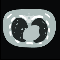
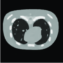
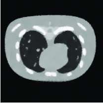
In this subsection, we apply the PD method stated in Section 2 to solve problem (2.3) on CT images and compare the results with the balanced approach (1.2) and the analysis based approach (1.3). The matrix $A$ in (1.1) is taken to be a projection matrix based on fan-beam scanning geometry using Siddon’s algorithm [49], and $\eta$ is generated from a zero mean Gaussian distribution with variance $\sigma=0.01\|f\|_{\infty}$. In addition, we pick level of framelet decomposition to be 4 for the best quality of the reconstructed images. For balanced approach, we set $\kappa=2$ and take ${\epsilon}_{P}=1.5\times 10^{-2}$ for the stopping criteria of the APG algorithm. We set ${\epsilon}_{S}=10^{-5}$ for the stopping criteria of the split Bregman algorithm when solving the analysis based approach. Moreover, we take ${\mathcal{Y}}=\{x\in{{\mathbb{R}}}^{n}:x_{i}\geq 0\ \forall i=1,\ldots,n\}$ for model (2.3), and take $\delta=10$ and ${\varrho}_{0}=10$ for the PD method. To measure quality of the restored image, we use the PSNR value defined by

$$\mbox{PSNR}:=-20\log_{10}\frac{\|u-{\tilde{u}}\|_{2}}{n},$$

where $u$ and ${\tilde{u}}$ are the original and restored images respectively, and $n$ is total number of pixels in $u$.

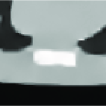
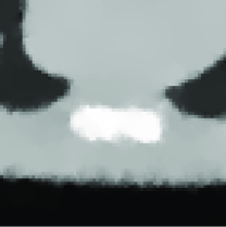
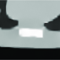
Table 1 summarizes the results of all three models when applying to the CT image restoration problem and the corresponding images and their zoom-in views are shown in Figure 1 and Figure 2. In Table 1, the CPU time (in seconds) and PSNR values of all three methods are given in the first and second row, respectively. In order to fairly compare the results, we have tuned the parameter $\lambda$ to achieve the best quality of the restoration images for each individual method. We observe that based on the PSNR values listed in Table 1 the analysis based approach and the PD method obviously achieve better restoration results than the balanced approach. Nevertheless, the APG algorithm for the balanced approach is the fastest algorithm in this experiment. In addition, the PD method is faster and achieves larger PSNR than the split Bergman algorithm for the analysis based approach. Moreover, we can observe from Figure 2 that the edges are recovered better by the PD method and the balanced approach.

Table 1. Comparisons: CT image reconstruction

	Balanced approach	Analysis based approach	PD method
Time	56.0	204.8	147.6
PSNR	56.06	59.90	60.22

Figure 1. CT image reconstruction. Images from left to right are: original CT image, reconstructed image by balanced approach, reconstructed image by analysis based approach and reconstructed image by PD method.

Figure 2. Zoom-in views of the CT image reconstruction. Images from left to right are: original CT image, reconstructed image by balanced approach, reconstructed image by analysis based approach and reconstructed image by PD method.

3.2. Experiments on image deconvolution

In this subsection, we apply the PD method stated in Section 2 to solve problem (2.3) on image deblurring problems and compare the results with the balanced approach (1.2) and the analysis based approach (1.3). The matrix $A$ in (2.3) is taken to be a convolution matrix with corresponding kernel a Gaussian function (generated in MATLAB by “fspecial(‘gaussian’,9,1.5);”) and $\eta$ is generated from a zero mean Gaussian distribution with variance $\sigma$. If not specified, we choose $\sigma=3$ in our experiments. In addition, we pick level of framelet decomposition to be 4 for the best quality of the reconstructed images. We set $\kappa=1$ for balanced approach and choose both ${\epsilon}_{P}$ and ${\epsilon}_{S}$ to be $10^{-4}$ for the stopping criteria of both APG algorithm and the split Bregman algorithm. Moreover, we set ${\mathcal{Y}}=\{x\in{{\mathbb{R}}}^{n}:0\leq x_{i}\leq 255\ \forall i=1,\ldots,n\}$ for model (2.3), and take $\delta=10$ and ${\varrho}_{0}=10^{-3}$ for the PD method. To measure quality of restored image, we use the PSNR value defined by

$$\mbox{PSNR}:=-20\log_{10}\frac{\|u-{\tilde{u}}\|_{2}}{255n}.$$

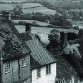
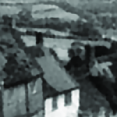
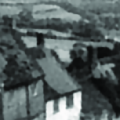
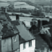
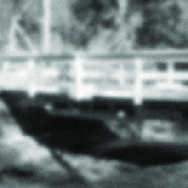
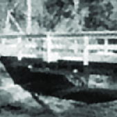
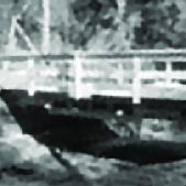
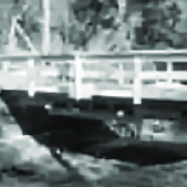
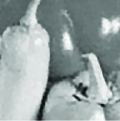
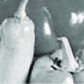
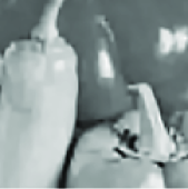
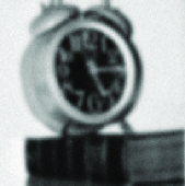
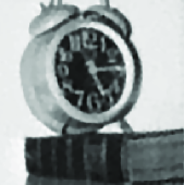
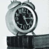
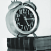
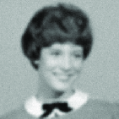
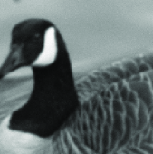
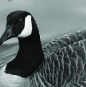
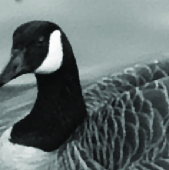
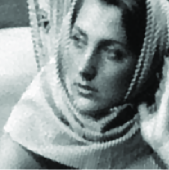
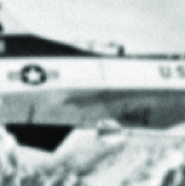
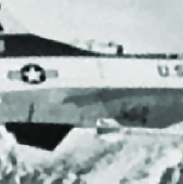
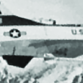
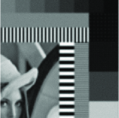
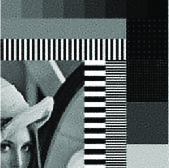
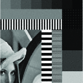
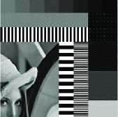
We first test all three methods on twelve different images by using piecewise linear wavelet and summarize the results in Table 2. The names and sizes of images are listed in the first two columns. The CPU time (in seconds) and PSNR values of all three methods are given in the rest six columns. In addition, the zoom-in views of original images, observed images and recovered images are shown in Figure 3-4. In order to fairly compare the results, we have tuned the parameter $\lambda$ to achieve the best quality of the restoration images for each individual method and each given image.

We first observe that in Table 2, the PSNR values obtained by the PD method are generally better than those obtained by other two approaches. Although for some of the images (i.e. “Downhill”, “Bridge”, “Duck” and “Barbara”), the PSNR values obtained by the PD methods are comparable to those of balanced and analysis based approaches, the quality of the restored images can not only be judged by their PSNR values. Indeed, the zoom-in views of the recovered images in Figure 3 and Figure 4 show that for all tested images, the PD method produces visually superior results than the other two approaches in terms of both sharpness of edges and smoothness of regions away from edges. Takeing the image “Barbara” as an example, the PSNR value of the PD method is only slightly greater than that obtained by the other two approaches. However, the zoom-in views of “Barbara” in Figure 4 show that the face of Barbara and the textures on her scarf are better recovered by the PD method than the other two approaches. This confirms the observation that penalizing $\ell_{0}$ “norm” of $Wu$ should provide good balance between sharpness of features and smoothness of the reconstructed images. We finally note that the PD method is slower than other two approaches in these experiments but the processing time of the PD method is still acceptable.

We next compare all three methods on “portrait I” image by using three different tight wavelet frame systems, i.e., Haar framelets, piecewise linear framelets and piecewise cubic framelets constructed by [44]. We summarize the results in Table 3. The names of three wavelets are listed in the first column. The CPU time (in seconds) and PSNR values of all three methods are given in the rest six columns. In Table 3, we can see that the quality of the restored images by using the piecewise linear framelets and the piecewise cubic framelets is better than that by using the Haar framelets. In addition, all three methods are generally faster when using Haar framelets and slower when using piecewise cubic framelets. Overall, all three approaches when using the piecewise linear have balanced performance in terms of time and quality (i.e., the PSNR value). Finally, we observe that the PD method consistently achieves the best quality of restored images among all the approaches for all three different tight wavelet frame systems.

Finally, we test how different noise levels affect the restored images obtained from all the three methods. We choose three different noise levels (i.e., $\sigma=3,5,7$) for image “Portrait I”, and test all the three methods by using piecewise linear framelets. We summarize the results in Table 4. The variances of noises are listed in the first column. The CPU time (in seconds) and PSNR values of all three methods are given in the rest six columns. We observe that the qualities of the restored images by all three methods degrade when the noise level increases. Nevertheless, the PD method still outperforms other two methods.

Figure 3. Zoom-in to the texture part of “downhill”, “cameraman”, “bridge”, “pepper”, “clock”, and “portrait I”. Image from left to right are: original image, observed image, results of the balanced approach, results of the analysis based approach and results of the PD method.

Figure 4. Zoom-in to the texture part of “duck”, “barbara”, “aircraft”, “couple”, “portrait II” and “lena”. Image from left to right are: original image, observed image, results of the balanced approach, results of the analysis based approach and results of the PD method.

Table 2. Comparisons: image deconvolution

		Balanced approach		Analysis based approach		PD method
Name	Size	Time	PSNR	Time	PSNR	Time	PSNR
Downhill	256	12.5	27.24	6.1	27.36	29.5	27.35
Cameraman	256	18.2	26.65	7.0	26.73	31.1	27.21
Bridge	256	14.5	25.40	5.1	25.46	33.0	25.44
Pepper	256	21.6	26.82	7.5	26.63	32.1	27.29
Clock	256	17.3	29.42	19.9	29.48	22.3	29.86
Portrait I	256	32.7	33.93	19.3	33.98	27.1	35.44
Duck	464	30.6	31.00	16.1	31.11	72.5	31.09
Barbara	512	38.8	24.62	12.3	24.62	77.4	24.69
Aircraft	512	55.9	30.75	35.1	30.81	67.5	31.29
Couple	512	91.4	28.40	41.5	28.14	139.1	29.32
Portrait II	512	45.2	30.23	22.1	30.20	48.9	30.90
Lena	516	89.3	12.91	31.0	12.51	67.0	13.45

Table 3. Comparisons among different wavelet representations

	Balanced approach		Analysis based approach		PD method
Wavelets	Time	PSNR	Time	PSNR	Time	PSNR
Haar	17.9	33.63	20.2	33.80	24.3	34.68
Piecewise linear	32.7	33.93	22.3	33.98	27.1	35.44
Piecewise cubic	61.0	33.95	37.3	34.00	37.8	35.20

Table 4. Comparisons among different noise levels for image “Portrait I”

	Balanced approach		Analysis based approach		PD method
Variances of noises	Time	PSNR	Time	PSNR	Time	PSNR
$\sigma=3$	32.7	33.93	22.3	33.98	27.1	35.44
$\sigma=5$	23.7	32.84	19.4	32.89	27.2	34.48
$\sigma=7$	19.6	32.11	25.0	32.14	29.7	33.69

4. Conclusion

In this paper, we proposed a wavelet frame based $\ell_{0}$ minimization model, which is motivated by the analysis based approach and balanced approach. The penalty decomposition (PD) method of [40] was used to solve the proposed optimization problem. Numerical results showed that the proposed model solved by the PD method can generate images with better quality than those obtained by either analysis based approach or balanced approach in terms of restoring sharp features like edges as well as maintaining smoothness of the recovered images. Convergence analysis of the sub-iterations in the PD method was also provided.

References

- [1] A. Antoniadis and J. Fan. Regularization of wavelet approximations. Journal of the American Statistical Association, 96(455):939–967, 2001.
- [2] G. Aubert and P. Kornprobst. Mathematical problems in image processing: partial differential equations and the calculus of variations. Springer, 2006.
- [3] A. Beck and M. Teboulle. A fast iterative shrinkage-thresholding algorithm for linear inverse problems. SIAM Journal on Imaging Sciences, 2(1):183–202, 2009.
- [4] E.G. Birgin, J.M. Martínez, and M. Raydan. Nonmonotone spectral projected gradient methods on convex sets. SIAM Journal on Optimization, 10(4):1196–1211, 2000.
- [5] T. Blumensath and M.E. Davies. Iterative thresholding for sparse approximations. Journal of Fourier Analysis and Applications, 14(5):629–654, 2008.
- [6] T. Blumensath and M.E. Davies. Iterative hard thresholding for compressed sensing. Applied and Computational Harmonic Analysis, 27(3):265–274, 2009.
- [7] J.F. Cai, R.H. Chan, L. Shen, and Z. Shen. Convergence analysis of tight framelet approach for missing data recovery. Advances in Computational Mathematics, 31(1):87–113, 2009.
- [8] J.F. Cai, R.H. Chan, and Z. Shen. Simultaneous cartoon and texture inpainting. Inverse Problems and Imaging, to appear, 2008.
- [9] J.F. Cai, B. Dong, S. Osher, and Z. Shen. Image restorations: total variation, wavelet frames and beyond. preprint, 2011.
- [10] J.F. Cai, S. Osher, and Z. Shen. Linearized Bregman iterations for frame-based image deblurring. SIAM Journal on Imaging Sciences, 2(1):226–252, 2009.
- [11] J.F. Cai, S. Osher, and Z. Shen. Split Bregman methods and frame based image restoration. Multiscale Modeling and Simulation: A SIAM Interdisciplinary Journal, 8(2):337–369, 2009.
- [12] E.J. Candes, Y.C. Eldar, D. Needell, and P. Randall. Compressed sensing with coherent and redundant dictionaries. Applied and Computational Harmonic Analysis, 2010.
- [13] E.J. Candès, J. Romberg, and T. Tao. Robust uncertainty principles: Exact signal reconstruction from highly incomplete frequency information. IEEE Transactions on Information Theory, 52(2):489–509, 2006.
- [14] E.J. Candes and T. Tao. Decoding by linear programming. IEEE Transactions on Information Theory, 51(12):4203–4215, 2005.
- [15] E.J. Candes and T. Tao. Near-optimal signal recovery from random projections: Universal encoding strategies? IEEE Transactions on Information Theory, 52(12):5406–5425, 2006.
- [16] A. Chai and Z. Shen. Deconvolution: A wavelet frame approach. Numerische Mathematik, 106(4):529–587, 2007.
- [17] A. Chambolle and P.L. Lions. Image recovery via total variation minimization and related problems. Numerische Mathematik, 76(2):167–188, 1997.
- [18] R.H. Chan, T.F. Chan, L. Shen, and Z. Shen. Wavelet algorithms for high-resolution image reconstruction. SIAM Journal on Scientific Computing, 24(4):1408–1432, 2003.
- [19] R.H. Chan, S.D. Riemenschneider, L. Shen, and Z. Shen. Tight frame: an efficient way for high-resolution image reconstruction. Applied and Computational Harmonic Analysis, 17(1):91–115, 2004.
- [20] R.H. Chan, L. Shen, and Z. Shen. A framelet-based approach for image inpainting. preprint, 4:325, 2005.
- [21] R.H. Chan, Z. Shen, and T. Xia. A framelet algorithm for enhancing video stills. Applied and Computational Harmonic Analysis, 23(2):153–170, 2007.
- [22] T. Chan, S. Esedoglu, F. Park, and A. Yip. Total variation image restoration: Overview and recent developments. Handbook of mathematical models in computer vision, pages 17–31, 2006.
- [23] T.F. Chan and J. Shen. Image processing and analysis: variational, PDE, wavelet, and stochastic methods. Society for Industrial Mathematics, 2005.
- [24] I. Daubechies. Ten lectures on wavelets, volume CBMS-NSF Lecture Notes, SIAM, nr. 61. Society for Industrial Mathematics, 1992.
- [25] I. Daubechies, B. Han, A. Ron, and Z. Shen. Framelets: MRA-based constructions of wavelet frames. Applied and Computational Harmonic Analysis, 14(1):1–46, 2003.
- [26] I. Daubechies, G. Teschke, and L. Vese. Iteratively solving linear inverse problems under general convex constraints. Inverse Problems and Imaging, 1(1):29–46, 2007.
- [27] B. Dong, A. Chien, and Z. Shen. Frame based segmentation for medical images. Communications in Mathematical Sciences, 9(2):551–559, 2010.
- [28] B. Dong and Z. Shen. MRA based wavelet frames and applications. IAS Lecture Notes Series, Summer Program on “The Mathematics of Image Processing”, Park City Mathematics Institute, 2010.
- [29] B. Dong and Z. Shen. Frame based surface reconstruction from unorganized points. accepted by Journal of Computational Physics, 2011.
- [30] D.L. Donoho. Compressed sensing. IEEE Transactions on Information Theory, 52:1289–1306, 2006.
- [31] M. Elad, J.L. Starck, P. Querre, and D.L. Donoho. Simultaneous cartoon and texture image inpainting using morphological component analysis (MCA). Applied and Computational Harmonic Analysis, 19(3):340–358, 2005.
- [32] M.J. Fadili and J.L. Starck. Sparse representations and bayesian image inpainting. Proceedings of SPARS, 2005.
- [33] M.J. Fadili, J.L. Starck, and F. Murtagh. Inpainting and zooming using sparse representations. The Computer Journal, 52(1):64, 2009.
- [34] M.A.T. Figueiredo and R.D. Nowak. An EM algorithm for wavelet-based image restoration. IEEE Transactions on Image Processing, 12(8):906–916, 2003.
- [35] M.A.T. Figueiredo and R.D. Nowak. A bound optimization approach to wavelet-based image deconvolution. IEEE International Conference on Image Processing, 2005.
- [36] D. Geman and C. Yang. Nonlinear image recovery with half-quadratic regularization. Image Processing, IEEE Transactions on, 4(7):932–946, 1995.
- [37] T. Goldstein and S. Osher. The split Bregman algorithm for L1 regularized problems. SIAM Journal on Imaging Sciences, 2(2):323–343, 2009.
- [38] K.K. Herrity, A.C. Gilbert, and J.A. Tropp. Sparse approximation via iterative thresholding. IEEE International Conference on Acoustics, Speech and Signal Processing, 2006.
- [39] X. Jia, Y. Lou, B. Dong, and S. Jiang. GPU-based iterative cone beam CT reconstruction using tight frame regularization. preprint, 2010.
- [40] Z. Lu and Y. Zhang. Penalty decomposition methods for -norm minimization. preprint, 2010.
- [41] Y. Meyer. Oscillating patterns in image processing and nonlinear evolution equations: the fifteenth Dean Jacqueline B. Lewis memorial lectures, volume 22. Amer Mathematical Society, 2001.
- [42] S. Osher and R.P. Fedkiw. Level set methods and dynamic implicit surfaces. Springer, 2003.
- [43] R.T. Rockafellar and J.B.W. Roger. Variational analysis, volume 317. Springer, 2004.
- [44] A. Ron and Z. Shen. Affine Systems in : The Analysis of the Analysis Operator. Journal of Functional Analysis, 148(2):408–447, 1997.
- [45] L. Rudin, S. Osher, and E. Fatemi. Nonlinear total variation based noise removal algorithms. Journal of Physics D, 60:259–268, 1992.
- [46] G. Sapiro. Geometric partial differential equations and image analysis. Cambridge Univ Pr, 2001.
- [47] Z. Shen. Wavelet frames and image restorations. Proceedings of the International Congress of Mathematicians, Hyderabad, India, 2010.
- [48] Z. Shen, K. C. Toh, and S. Yun. An accelerated proximal gradient algorithm for frame based image restorations via the balanced approach. SIAM Journal on Imaging Sciences, 4(2):573–596, 2011.
- [49] R.L. Siddon. Fast calculation of the exact radiological path for a three-dimensional CT array. Medical Physics, 12:252–255, 1985.
- [50] J.L. Starck, M. Elad, and D.L. Donoho. Image decomposition via the combination of sparse representations and a variational approach. IEEE Transactions on Image Processing, 14(10):1570–1582, 2005.
- [51] G. Steidl, J. Weickert, T. Brox, P. Mrázek, and M. Welk. On the equivalence of soft wavelet shrinkage, total variation diffusion, total variation regularization, and sides. SIAM Journal on Numerical Analysis, pages 686–713, 2005.
- [52] P. Tseng. Convergence of a block coordinate descent method for nondifferentiable minimization. Journal of optimization theory and applications, 109(3):475–494, 2001.
- [53] Y. Wang, J. Yang, W. Yin, and Y. Zhang. A new alternating minimization algorithm for total variation image reconstruction. SIAM Journal on Imaging Sciences, 1(3):248–272, 2008.