Bayesian analysis of variable-order, reversible Markov chains

Abstract

We define a conjugate prior for the reversible Markov chain of order $r$. The prior arises from a partially exchangeable reinforced random walk, in the same way that the Beta distribution arises from the exchangeable Polyá urn. An extension to variable-order Markov chains is also derived. We show the utility of this prior in testing the order and estimating the parameters of a reversible Markov model.

T1Supported by a Smith Stanford Graduate Fellowship and Grants NIH-R01-GM062868 and NSF DMS-09-00700.

1 Introduction

Reversible Markov chains are central to a number of fields. They underlie problems in applied probability like card-shuffling and queueing networks AldousFill , Kelly1979fv and pervade computational statistics through the many variants of Markov chain Monte Carlo; in physics, they are natural stochastic models for time-reversible dynamics. However, the notion of reversibility in stochastic proscesses with memory is not as widely discussed, and statistical problems like testing the order of a reversible process remain a challenge.

We define a conjugate prior for higher-order, reversible Markov chains, which extends a prior for reversible Markov chains by Diaconis and Rolles Diaconis2006gd . We begin by defining reversibility in a more general setting and motivating the significance of higher-order processes. In Section 2, we present two graphical representations for an order-$r$, reversible Markov chain, which are used in Section 3 to derive the conjugate prior via a random walk with reinforcement. We dedicate Section 4 to variable-order Markov chains, a family of models that avoids the curse of dimensionality associated with higher-order Markov chains, proving essential in certain applications. Finally in Section 5, we discuss properties of the prior pertaining to Bayesian analysis. In examples, we test the extent of memory of a lumped Markov chain and discretized molecular dynamics trajectories, and compare the posterior inferences of different models.

Definition 1.1.

A stochastic process $X=X_{n},n\in\mathbb{N}$, with distribution $P$ is called reversible, if for any $m>n>0$,

$$P(X_{1},X_{2},\ldots,X_{n})=P(X_{m-1},X_{m-2},\ldots,X_{m-n}).$$

It is not difficult to show that reversibility implies stationarity Kelly1979fv ; if stationarity is given, the above condition need only be checked for $m=n+1$. Now suppose $X$ is an order-$r$, irreducible Markov chain taking values in a finite set $\mathcal{X}$. We will also apply the term reversible to this process when the stationary chain satisfies the reversibility condition.

Proposition 1.2.

Let $P$ be the stationary law of the order-$r$ Markov chain $X$. If $P(X_{1},\ldots,X_{r+1})=P(X_{r+1},\ldots,X_{1})$, then the Markov chain is reversible.

It is not difficult to check that the hypothesis together with stationarity imply $P(X_{1},\ldots,X_{n})=P(X_{n},\ldots,X_{1})$ for any $n<r+1$. For any $n>r+1$:

$$P(X_{1},\ldots,X_{n}) = P(X_{1},\ldots,X_{r+1})\prod_{i=r+2}^{n}P(X_{i}|X_{i-r},\ldots,X_{i-1})$$

$$= P(X_{1},\ldots,X_{r+1})\frac{P(X_{2},\ldots,X_{r+2})}{P(X_{2},\ldots,X_{r+1})}\cdots\frac{P(X_{n-r},\ldots,X_{n})}{P(X_{n-r},\ldots,X_{n-1})}$$

$$= P(X_{n},\ldots,X_{n-r})\frac{P(X_{n-1},\ldots,X_{n-r-1})}{P(X_{n-1},\ldots,X_{n-r})}\cdots\frac{P(X_{r+1},\ldots,X_{1})}{P(X_{r+1},\ldots,X_{2})}$$

$$= P(X_{n},\ldots,X_{1}),$$

where we have used the Markov property, stationarity and the hypothesis.

As a first remark, note that $X_{n},n\in\mathbb{N}$, can be represented as a first-order Markov chain $V_{n},n\in\mathbb{N}$, taking values in the space of sequences $\mathcal{X}^{r}$. However, the reversibility of $X$ does not imply the reversibility of its first-order representation; therefore, the analysis of higher-order reversible Markov chains requires novel techniques. In the following sections, we often use the first-order representation $V_{n},n\in\mathbb{N}$, referring to it nonetheless as an order-$r$ Markov chain and using the notion of reversibility associated with the order-$r$ Markov chain.

Secondly, we recall that Kolmogorov’s criterion is another necessary and sufficient condition for the reversibility of a Markov chain, which only depends on the conditional transition probabilities Kelly1979fv . Its equivalence to Definition 1.1 in the higher-order case is proven in the Appendix. Kolmogorov’s criterion requires that the probability of traversing any cycle in either direction is the same. Accordingly, a reversible Markov chain can be interpreted as a process with no net circulation in space.

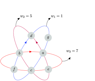
Figure 1: A set of weighted circuits on the set $\mathcal{X}=\{a,b,c,d,e,f,g\}$. In a circuit process started at $u$ in $\mathcal{X}^{r}$, we transition on some circuit that contains $u$ with probability proportional to its weight.

Reversibility is preserved under certain transformations. For example, let $X_{n},n\in\mathbb{N}$, be a stationary, reversible Markov chain and consider a finitely valued function, $f(X_{n}),n\in\mathbb{N}$. It is easy to check that this process is stationary and reversible, even though it may not be a Markov chain of any finite order. Functions or projections of reversible Markov chains appear under different guises in physics and other fields, and in many cases the effects of memory subside with time, motivating the use of finite order models. The problems of determining the order and estimating the parameters of Markov models have been studied extensively; here, we address these problems with the constraint of reversibility.

2 Graphical representations of reversible Markov chains

For any sequence $u\in\mathcal{X}^{s}$, let $u^{*}$ be its inverse, $\mathrm{A}(u)$ the subsequence obtained by deleting its last element and $\Omega(u)$ the one obtained by deleting its first element. We call $u_{1},u_{2},\ldots,u_{n}$ with $u_{i}\in\mathcal{X}^{s}$ an admissible path if $\Omega(u_{i})=\mathrm{A}(u_{i+1})$ for all $1\leq i<n$. The concatenation of these sequences without repeated overlaps is denoted $\overline{u_{1}\cdots u_{n}}\in\mathcal{X}^{s+n-1}$.

The first representation we will consider is the circuit process of MacQueen MacQueen1981df . Let a circuit be a periodic function on $\mathcal{X}$, and consider a class of positively weighted circuits $\mathscr{C}$ (for an example, see Figure 1).

Definition 2.1.

A circuit process of order $r$ is a Markov chain of the same order, where the transition probability from $u\in\mathcal{X}^{r}$ to any $v\in\mathcal{X}^{r}$ with $\Omega(u)=\mathrm{A}(v)$ is given by

$$\frac{\sum_{\gamma\in\mathscr{C}}w_{\gamma}J_{\gamma}(\overline{uv})}{\sum_{\gamma\in\mathscr{C}}w_{\gamma}J_{\gamma}(u)},$$

where $w_{\gamma}>0$ is the weight of circuit $\gamma$, and the function $J_{\gamma}(\cdot)$ counts the number of times that the circuit traverses a sequence in one period. In other words, in each step we move along some circuit in $\mathscr{C}$ containing the current state with probability proportional to its weight. The process only visits states that appear in the circuits, for which transition probabilities are well defined.

An irreducible order-$r$ Markov chain with stationary law $P_{\pi}$ is parametrized by $P_{\pi}(u)$ for all $u\in\mathcal{X}^{r+1}$. One can check that in a circuit process, this is just $P_{\pi}(u)=\sum_{\gamma\in\mathscr{C}}w_{\gamma}J_{\gamma}(u)$. MacQueen showed that any order-$r$ Markov chain can be represented as a circuit process on a finite set $\mathscr{C}$, which is not unique MacQueen1981df . This is true in particular when the chain is reversible.

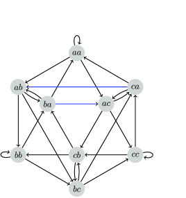
Figure 2: A de Bruijn graph of order 2 on the state space $\mathcal{X}=\{a,b,c\}$. In a reversible random walk, the two highlighted edges have the same weight.

We introduce a second graphical representation that is canonical, unlike the circuit process. Consider a de Bruijn graph on the vertices $\mathcal{X}^{r}$, which has a directed edge from $u$ to $v$ if and only if $\Omega(u)=\mathrm{A}(v)$. That is, every path on the graph is an admissible path. For an example, see Figure 2. Assign a weight $k_{uv}\geq 0$ to each edge, and let $k_{u}$ be the summed weights of edges departing from $u$. Furthermore, require that

$$k_{uv} = k_{v^{*}u^{*}}\qquad\mbox{for every edge }uv,$$ (1)

$$k_{u} = k_{u^{*}}\qquad\mbox{for all }u\in\mathcal{X}^{r}\quad\mbox{and}$$ (2)

$$\sum_{u\in\mathcal{X}^{r}}k_{u} = 1.$$ (3)

Definition 2.2.

The reversible random walk of order $r$ is a random walk on such a graph, with transition probabilities

$$p(v|u)=\frac{k_{uv}}{k_{u}}.$$

Proposition 2.3.

An irreducible, reversible random walk of order $r$ represents a reversible Markov chain of the same order. Every irreducible, reversible order-$r$ Markov chain is equivalent to a unique reversible random walk of order $r$.

Let $\pi$ be the stationary distribution of the random walk. To prove the first statement, we will first verify that $\pi(u)=k_{u}$ for all $u\in\mathcal{X}^{r}$. Let $p(u|v)$ be the transition probability from $v$ to $u$ in the random walk, and recall that $\Omega(u)=\mathrm{A}(v)$ iff $\Omega(v^{*})=\mathrm{A}(u^{*})$, then

$$\sum_{u\in\mathcal{X}^{r}}\pi(u)p(v|u) = \sum_{\{u\in\mathcal{X}^{r}\dvtx\Omega(u)=\mathrm{A}(v)\}}k_{u}\frac{k_{uv}}{k_{u}}$$

$$= \sum_{\{u\in\mathcal{X}^{r}\dvtx\Omega(v^{*})=\mathrm{A}(u^{*})\}}k_{v^{*}u^{*}}=k_{v^{*}}=k_{v}=\pi(v).$$

Then, the stationary law $P_{\pi}$ in the random walk of a path $u,v$ is just

$$P_{\pi}(u,v)=\pi(u)p(v|u)=k_{u}\frac{k_{uv}}{k_{u}}=k_{uv},$$

which implies that $P_{\pi}(u,v)=k_{uv}=k_{v^{*}u^{*}}=P_{\pi}(v^{*},u^{*})$. Therefore, the $\mathcal{X}$-valued, order-$r$ Markov chain represented by the random walk satisfies the reversibility condition in Proposition 1.2. Proving the second statement is now straightforward. Let $V_{n},n\in\mathbb{N}$, be the first-order representation of an irreducible, order-$r$ Markov chain, with transition probabilities $p^{\prime}(v|u)$. By the Perron–Frobenius theorem, $V$ has a unique stationary distribution $\pi^{\prime}$. Assign edge weights to the de Bruijn graph on $\mathcal{X}^{r}$, setting $k_{uv}=\pi^{\prime}(u)p^{\prime}(v|u)$. Since the order-$r$ Markov chain is reversible, it follows directly from Proposition 1.2 that the edge weights satisfy conditions (1)–(3).

3 From a reinforced random walk to the conjugate prior

An edge-reinforced random walk (ERRW) is a random walk on an finite, undirected graph, where every edge-weight is increased by 1 each time it is crossed. Since Diaconis and Coppersmith defined this process Diaconis1988 , we have learned that it is partially exchangeable and, by de Finetti’s theorem for Markov chains, a mixture of Markov chains Diaconis1980hb . The mixing measure, which lives on the space of reversible Markov chains, was more recently characterized in the literature Keane2000df . Diaconis and Rolles showed that this distribution is a conjugate prior for the reversible Markov chain, much as the Beta distribution, arising from a Polyá urn scheme, is a conjugate prior for sequences of i.i.d. binary random variables Diaconis2006gd .

Here, we construct a conjugate prior for higher-order reversible Markov chains via a reinforced random walk in $\mathcal{X}^{r}$, making use of de Finetti’s theorem for Markov chains. This process is markedly different from an ERRW in $\mathcal{X}^{r}$ due to the structure of a reversible Markov chain with memory, although it is designed to be partially exchangeable.

Let $\alpha$ be any sequence on $\mathcal{X}$ and $v$ a sequence shorter than $\alpha$. Define the function $J^{\prime}_{\alpha}(v)$, which counts the number of times that $v$ appears in $\alpha$, and $J^{\prime\prime}_{\alpha}(v)$, which counts the number of times that $v$ appears in $\alpha$ followed by at least one state. Fix $w$, a stationary measure for an irreducible, reversible, order-$r$ Markov chain. Also fix $v_{0}\in\mathcal{X}^{r}$. Let $\beta$ be a palindromic sequence that starts with $v_{0}$ and ends with $v_{0}^{*}$. Choose a positive constant $c$, such that for all $u\in\mathcal{X}^{r+1}$, $w(u)-cJ^{\prime}_{\beta}(u)>0$. Now, given a sequence $\eta$, starting with $v_{0}$, and any sequence $v$, define the functions

$$w^{\prime}(\eta,v) = w(v)+c\bigl{(}J^{\prime}_{\eta}(v)+J^{\prime}_{\eta^{*}}(v)-J^{\prime}_{\beta}(v)\bigr{)}\quad\mbox{and}$$ (4)

$$w^{\prime\prime}(\eta,v) = w(v)+c\bigl{(}J^{\prime\prime}_{\eta}(v)+J^{\prime\prime}_{\eta^{*}}(v)-J^{\prime\prime}_{\beta}(v)\bigr{)}.$$ (5)

When $\eta$ represents the path of a stochastic process in $\mathcal{X}^{r}$ up to time $n$ (formally, $\eta=\overline{v_{0}\cdots v_{n}}$), we will use the notation $w^{\prime}_{n}(v)\equiv w^{\prime}(\eta,v)$ and $w^{\prime\prime}_{n}(v)\equiv w^{\prime\prime}(\eta,v)$.

Definition 3.1.

The reinforced random walk of order $r$ is a stochastic process $Y_{n},n\in\mathbb{N}$, on $\mathcal{X}^{r}$ with distribution $Q_{w,v_{0}}$. The initial state is $v_{0}$ with probability 1. For any admissible path $v_{0},\ldots,v_{n}$, the conditional transition probability

$$Q_{w,v_{0}}(Y_{n+1}=u|Y_{0}=v_{0},\ldots,Y_{n}=v_{n})=\frac{w^{\prime}_{n}(\overline{v_{n}u})}{w^{\prime\prime}_{n}(v_{n})}$$

whenever $v_{n},u$ is admissible and zero otherwise.

Remark 3.2.

The law $Q_{w,v_{0}}$ also depends on $\beta$ and $c$. These parameters are constant in the following discussion, so they are omitted from the notation for conciseness. When $r=1$, this process is equivalent to an ERRW. In this case, the palindrome is unnecessary because the terms involving $\beta$ in $w^{\prime}$ and $w^{\prime\prime}$ can be modeled with a different $w$. For $r\geq 2$, this is not the case, and $\beta$ is essential for partial exchangeability (see Proposition 3.5).

Remark 3.3.

This process admits an interpretation as a reinforcement scheme of the circuit process. Consider a circuit process of order $r$ with stationary probability $w(u)=\sum_{\gamma\in\mathscr{C}}w_{\gamma}J_{\gamma}(u)$ for all $u\in\mathcal{X}^{r+1}$. In addition, consider three weighted sequences: the palindrome $\beta$, a sequence $\eta$ that represents the path of the reinforced process from the initial state $v_{0}$ up to the current state, and the reversed path $\eta^{*}$. These are depicted in Figure 3 along with their weights $-c$, $c$ and $c$, respectively. As in the circuit process, we move along any circuit or sequence that contains the current state with probability proportional to its weight. The reinforcement is accomplished by elongating the paths $\eta$ and $\eta^{*}$.

Remark 3.4.

The process is also a reinforcement scheme of a modified reversible random walk of order $r$. Consider a weighted de Bruijn graph, where for every admissible $u,v$, $k_{uv}=w(\overline{uv})$. Then, for every $\overline{uv}$ in the palindrome $\beta$, subtract $c$ from $k_{uv}$. The reinforcement scheme will consist of a random walk on the resulting graph, where after every transition $v_{i}\to v_{i+1}$ we increase both $k_{v_{i}v_{i+1}}$ and $k_{v_{i+1}^{*}v_{i}^{*}}$ by $c$. Accordingly, if $\overline{v_{i}v_{i+1}}$ is a palindrome, the weight $k_{v_{i}v_{i+1}}$ is increased by $2c$.

Proposition 3.5.

The reinforced random walk of order $r$ is partially exchangeable in the sense of Diaconis and Freedman Diaconis1980hb .

We must show that the probability $Q_{w,v_{0}}(v_{0},\ldots,v_{n})$ of any admissible path $v_{0},\ldots,v_{n}$ is a function of the initial state $v_{0}$ and the transition counts between every pair of states. For any pair $u,v$ in $\mathcal{X}^{r}$ with $\mathrm{A}(v)=\Omega(u)$, let $C(u,v)$ be the total number of transitions $u\to v$, and $v^{*}\to u^{*}$. We will show the stronger statement that $v_{0}$ and $C$ are sufficient statistics for the reinforced random walk.

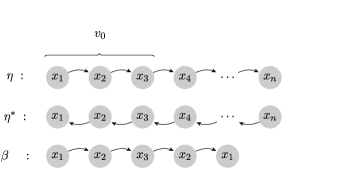
Figure 3: Auxiliary sequences in the order-$r$ reinforced random walk.

Let us first establish some properties that are conserved in the process. For every $u\in\mathcal{X}^{r+1}$, the initial weights $w^{\prime}_{0}(u)$ and $w^{\prime}_{0}(u^{*})$ are equal. This is direct from the definition in equation (4) because: $w$ defines a reversible Markov chain of order $r$; the functions $J_{v_{0}}^{\prime}$ and $J_{v_{0}^{*}}^{\prime}$ are zero for both $u$ and $u^{*}$; and $\beta$ is a palindrome, so if it contains $u$, it also contains $u^{*}$, and $J_{\beta}^{\prime}(u)=J_{\beta}^{\prime}(u^{*})$. This property is maintained after every transition $v_{n}\to v_{n+1}$, because the weights may both be increased by $c$ if $\overline{v_{n}v_{n+1}}$ is $u$ or $u^{*}$, or both remain constant otherwise.

For every $v\neq v_{0}$ in $\mathcal{X}^{r}$, the initial weights $w^{\prime\prime}_{0}(v)=w^{\prime\prime}_{0}(v^{*})$. This is direct from equation (5) because: $w$ is reversible, both $J_{v_{0}}^{\prime\prime}$ and $J_{v_{0}^{*}}^{\prime\prime}$ are zero for $v$ and $v^{*}$, and the sequence $\beta$ is a palindrome, so for every transition starting at $v$ there will be another starting from $v^{*}$. The last fact is not necessarily true for $v_{0}$, because unless $v_{0}$ itself is a palindrome, $\beta$ will contain a transition starting from it, but no transition starting from $v_{0}^{*}$. So, in the beginning, $w^{\prime\prime}_{0}(v_{0})=w^{\prime\prime}_{0}(v_{0}^{*})-c$. When a transition occurs from $v_{0}$ to $v_{1}$, the weights $w^{\prime\prime}_{1}(v_{0})$ and $w^{\prime\prime}_{1}(v_{0}^{*})$ become equal, while $w^{\prime\prime}_{1}(v_{1})=w^{\prime\prime}_{1}(v_{1}^{*})-c$, provided $v_{1}$ is not a palindrome. Hence, this singularity is preserved by the last state visited by the process.

The probability $Q_{w,v_{0}}(v_{0},\ldots,v_{n})$ is a ratio of two products. In the numerator, we find a factor of the form $w^{\prime}_{t}(\overline{uv})$ for every admissible transition $u\to v$, while in the denominator, we find a corresponding weight $w^{\prime\prime}_{t}(u)$. It is easy to check that the numerator is only a function of $C$. Every transition $u\to v$ or $v^{*}\to u^{*}$ adds a new factor of $w^{\prime}_{t}(\overline{uv})$, which is always greater than the previous one by $c$. If $\overline{uv}$ is a palindrome, then every new factor of $w^{\prime}_{t}(\overline{uv})$ is increased by $2c$. So, the numerator can be computed from the initial weights and $C$.

We have left to show that the denominator is only dependent on $v_{0}$ and $C$. Note that the transition counts from $v$ or $v^{*}$ are a function of $C$ and $v_{0}$, because every event $v\to u$ is a transition from $v$, while every event $u^{*}\to v^{*}$ is followed by a transition from $v^{*}$, unless this is the final state, which is determined by $v_{0}$. After every transition from $v$ or $v^{*}$, we add a factor of $w_{t}^{\prime\prime}(v)$ or $w^{\prime\prime}_{t}(v^{*})$ to the denominator. At any time $t$, these weights differ by $c$ (if $v$ is not a palindrome), but the factor added is always the smaller of the two. Between two transitions, each of these weights is reinforced by $c$, so consecutive factors differ by that amount. If $v$ is a palindrome, there is no distinction between $w^{\prime\prime}_{t}(v)$ and $w^{\prime\prime}_{t}(v^{*})$, and consecutive factors differ by $2c$.

Lemma 3.6.

Suppose that in the reinforced random walk, we visit $v$ and $v^{*}$ in $\mathcal{X}^{r}$ infinitely often a.s., and let $\tau_{n}$ be the $n$th time we visit either state. The process $Y_{\tau_{n}}$ is a mixture of Markov chains. Furthermore, if $D_{n}$ is the ratio of the number of visits to $v^{*}$ and $v$ by $\tau_{n}$, $D_{n}$ converges a.s. to a finite limit $D_{\infty}$.

We claim that if $Y_{n}$ is partially exchangeable, so is $Y_{\tau_{n}}$. It is sufficient to show that the probability of a sequence $Y_{\tau_{n}}$ is invariant upon block transpositions, which generate the group of permutations that preserve transition counts (Diaconis1980hb , Proposition 27). The probability of a path $v_{\tau_{1}},\ldots,v_{\tau_{n}}$ in $Y_{\tau_{n}}$ is the sum of the probabilities of all paths $v_{0},v_{1},\ldots,v_{\tau_{n}}$ in $Y_{n}$ that map to it. Denote this set of paths $\Theta$. After a transposition of $v$-blocks or $v^{*}$-blocks, the probability of the path in $Y_{\tau_{n}}$ is equal to the sum of the probabilities of a different set of paths $\Theta^{\prime}$ in $Y_{n}$. However, it is easy to see that this transpostion of $v$-blocks or $v^{*}$-blocks defines a bijection from $\Theta$ to $\Theta^{\prime}$, and the probability of each path and its transposition is the same, because $Y_{n}$ is partially exchangeable. Therefore, $Y_{\tau_{n}}$ is partially exchangeable. Furthermore, we assume that $v$ and $v^{*}$ are recurrent, so by de Finetti’s theorem for Markov chains $Y_{\tau_{n}}$ is a mixture of Markov chains with a unique measure $\mu$ on the space of 2 by 2 transition matrices Diaconis1980hb . Note that both states are recurrent with probability 1, so the subset of transition matrices where one of the states is transient has $\mu$-measure zero. This implies that $\mu$-a.s. the transition matrix is irreducible, and since the state space is finite, both states are positive-recurrent. Therefore, $D_{n}$ converges a.s. to a finite limit.

Proposition 3.7.

The reinforced random walk of order $r$ traverses every edge $v\to u$ with $w(\overline{uv})>0$ infinitely often, almost surely.

As $\mathcal{X}$ is finite, we must visit at least one state in $\mathcal{X}^{r}$ infinitely often, so without loss of generality, let this state be $v$. Let $\tau_{n}$ be the $n$th time we visit $v$, and $\mathcal{F}_{n}$ be $\sigma(Y_{1},\ldots,Y_{\tau_{n}})$. For $u$ with $v,u$ admissible and $w(\overline{vu})>0$, let $A_{n}$ be the event that $Y_{\tau_{n}+1}=u$. Also, let $p_{n}=Q_{w,v_{0}}(A_{n}|\mathcal{F}_{n})$. By Lévy’s extension of the Borel–Cantelli lemma (Lemma .2),

$$\lim_{n\to\infty}\frac{\sum_{m=1}^{n}1_{A_{m}}}{\sum_{m=1}^{n}p_{m}}=1\qquad\mbox{on }\Biggl{\{}\sum_{m=1}^{\infty}p_{m}=\infty\Biggr{\}}.$$

Therefore, to show that the transition $v\to u$ is observed infinitely often with probability 1, it is sufficient to show that $\sum_{m}p_{m}=\infty$ a.s. The conditional probability $p_{m}$ is just $w^{\prime}_{\tau_{m}}(\overline{vu})/w_{\tau_{m}}^{\prime\prime}(v)$. Let $B_{m,k}$ be the event that we observe $v^{*}$ fewer than $km$ times between $\tau_{1}$ and $\tau_{m}$. On $B_{m,k}$, we can lower-bound $p_{m}$ using the minimum possible value of $w^{\prime}_{\tau_{m}}(\overline{vu})$, which is its initial value, and the maximum possible value of $w^{\prime\prime}_{\tau_{m}}(v)$, which is $(k+1)mc$. Thus,

$$p_{m} = Q_{w,v_{0}}(A_{m}\cap B_{m,k}|\mathcal{F}_{n})+Q_{w,v_{0}}(A_{m}\cap B_{m,k}^{C}|\mathcal{F}_{n})$$

$$\geq \mathbf{1}_{B_{m,k}}\frac{w^{\prime}_{\tau_{1}}(\overline{vu})}{(k+1)mc}.$$

Now, consider the event $\{D_{\infty}<N\}$. On this set, for any $k>N$, we will be in $B_{m,k}$ for all but finitely many $m$, which implies $\sum_{m}p_{m}=\infty$, by the previous inequality. But, by Lemma 3.6 we have $Q_{w,v_{0}}\{D_{\infty}<\infty\}=1$, so noting $\{D_{\infty}<\infty\}=\bigcup_{N\in\mathbb{N}}\{D_{\infty}<N\}$ we conclude that $\sum_{m}p_{m}=\infty$ $Q_{w,v_{0}}$-a.s., and $A_{m}$ happens infinitely often. Since $w$ defines an irreducible Markov chain, the proposition follows by induction.

Propositions 3.7 and 3.5 are sufficient to show by de Finetti’s theorem for Markov chains Diaconis1980hb that the reinforced random walk of order $r$ is a mixture of Markov chains on $\mathcal{X}^{r}$, or

$$Q_{w,v_{0}}(v_{0},\ldots,v_{n})=\int_{\mathcal{T}}P_{v_{0}}^{T}(v_{0},\ldots,v_{n})\,d\phi_{w,v_{0}}(T),$$ (6)

where $P_{v_{0}}^{T}$ is the distribution of a Markov chain started at $v_{0}$ and parametrized by the matrix $T$, $\mathcal{T}$ is the space of $\mathcal{X}^{r}\times\mathcal{X}^{r}$ stochastic matrices and $\phi_{w,v_{0}}$ is a unique measure on the Borel subsets of this space. Let $\mathcal{T^{\prime}}\subseteq\mathcal{T}$ be the set of matrices that represent irreducible, reversible Markov chains of order $r$.

Proposition 3.8.

The reinforced random walk of order $r$ is a mixture of reversible Markov chains of the same order, or $\phi_{w,v_{0}}(\mathcal{T}^{\prime})=1$.

This is a special case of Proposition 4.6.

4 Variable-order, reversible Markov chains

The number of parameters of a Markov chain grows as $|\mathcal{X}|^{r}$ with the order, $r$, which renders higher-order models impractical in many statistical applications. In this section, we investigate a family of models with finite memory length which do not suffer from this curse of dimensionality.

Definition 4.1.

A variable-order Markov chain is a Markov chain of order $r$ with the constraint that for every history $h$ in the set $\mathscr{H}\subseteq\{v\in\mathcal{X}^{q}\dvtx q<r\}$, if two states $u,u^{\prime}\in\mathcal{X}^{r}$ both end in $h$, the transition probabilities $p(v|u)$ and $p(v|u^{\prime})$ are equal for every $v\in\mathcal{X}^{r}$.

In essence, this is a discrete process which upon reaching a sequence $h\in\mathscr{H}$ loses memory of what preceded it. When $\mathscr{H}$ is empty, we recover a general Markov chain of order $r$. Variable-order Markov chains have proven useful in applications where there is long memory only in certain directions. The literature on the subject can be traced to Rissanen Rissanen1983 and Weinberger Weinberger1995 , who developed tree-based algorithms for estimating the set of histories efficiently in the context of compression. Bühlmann and Wyner proved several consistency results on these algorithms Buhlmann1999 , and the former later addressed the problem of model selection Buhlmann2000 . For an evaluation of different algorithms in applications, see Begleiter2004 .

It is worth noting that MacQueen mentioned variable-order Markov chains in an unpublished abstract. However, there is a marked difference between his definition and Bühlmann and Wyner’s, which relates to the closure properties of $\mathscr{H}$. MacQueen requires that if $h$ is in $\mathscr{H}$, then so are all the sequences that begin with $h$. Intuitively, this means that the process cannot recover memory once it is lost. Bühlmann and Wyner do not impose this constraint. However, this is guaranteed when the process is reversible.

Proposition 4.2.

Let $X_{n},n\in\mathbb{N}$, be an irreducible, reversible, variable-order Markov chain with histories $\mathscr{H}$. If $h\in\mathscr{H}$, then $h^{*}$ is also a history; additionally, any sequence that has $h$ as a prefix is also in $\mathscr{H}$.

Let $P_{\pi}$ be the stationary law of the chain. If $h\in\mathscr{H}$, then for any pair $a,b\in\mathcal{X}^{q}$, where $q$ and the length of $h$ sum to $r$, $P_{\pi}(X_{1},\ldots,X_{r+q}=ahb|X_{1},\ldots,X_{r}=ah)$ is independent of $a$, or

$$\frac{P_{\pi}(ahb)}{P_{\pi}(ah)}=C\qquad\forall a\in\mathcal{X}^{q}.$$

This implies

$$\frac{P_{\pi}(hb)}{P_{\pi}(h)}=\frac{\sum_{a\in\mathcal{X}^{q}}P_{\pi}(ahb)}{\sum_{a\in\mathcal{X}^{q}}P_{\pi}(ah)}=\frac{\sum_{a\in\mathcal{X}^{q}}P_{\pi}(ah)C}{\sum_{a\in\mathcal{X}^{q}}P_{\pi}(ah)}=\frac{P_{\pi}(ahb)}{P_{\pi}(ah)}.$$

Using the fact that $P_{\pi}$ is invariant upon time reversal and rearranging factors, we obtain

$$\frac{P_{\pi}(b^{*}h^{*}a^{*})}{P_{\pi}(b^{*}h^{*})}=\frac{P_{\pi}(h^{*}a^{*})}{P_{\pi}(h^{*})}.$$

The left-hand side is equal to $P_{\pi}(X_{1},\ldots,X_{r+q}=b^{*}h^{*}a^{*}|X_{1},\ldots,X_{r}=b^{*}h^{*})$, which by the previous identity is independent of $b^{*}$. As this is true for any $a\in\mathcal{X}^{q}$, $h^{*}$ must be a history in $\mathscr{H}$. To prove the second part of the statement, suppose $h$ is a prefix of $g$. Since $h^{*}$ is in $\mathscr{H}$, and $g^{*}$ ends in $h^{*}$, then by definition $g^{*}\in\mathscr{H}$. Using the first result, we conclude that $g\in\mathscr{H}$.

We will define a reinforcement scheme, which like the one in the previous section is recurrent, partially exchangeable and, by de Finetti’s theorem, a mixture of Markov chains. But, in this case, the mixing measure is restricted to the variable-order, reversible Markov chains with a fixed set of histories $\mathscr{H}$. As before, we begin with a stationary, reversible function $w$, an initial state $v_{0}\in\mathcal{X}^{r}$, and a palindromic sequence $\beta$ that starts with $v_{0}$. Let the function $f\dvtx\mathcal{X}^{r}\mapsto\mathscr{H}$ map any sequence to its shortest ending in $\mathscr{H}$.

Definition 4.3.

The variable-order, reinforced random walk is a stochastic process $Z_{n},n\in\mathbb{N}$, on $\mathcal{X}^{r}$ with measure $H_{w,v_{0}}$. The initial state is $v_{0}$ with probability 1. For any admissible path $v_{0},\ldots,v_{n}$, the conditional transition probability

$$H_{w,v_{0}}(Z_{n+1}=u|Z_{0}=v_{0},\ldots,Z_{n}=v_{n})=\frac{w^{\prime}_{n}(\overline{f(v_{n})u})}{w^{\prime\prime}_{n}(f(v_{n}))}$$

whenever $v_{n},u$ is admissible and zero otherwise.

Remark 4.4.

This process is a reinforced circuit process, just like the one defined in Remark 3.3, with the difference that in computing the transition probabilities, instead of taking the current state to be the sequence $v_{n}\in\mathcal{X}^{r}$, we let it be the shortest ending of $v_{n}$ in $\mathscr{H}$, or $f(v_{n})$.

Proposition 4.5.

The variable-order, reinforced random walk is partially exchangeable in the sense of Diaconis and Freedman.

This proof is deferred to the Appendix. One can show that this process is recurrent following the same argument of Proposition 3.7. In the proof of Proposition 3.7, we use a shortest history $h$ in place of $v$, and Lemma 3.6 still holds for $h$ and $h^{*}$. Recurrence and partial exchangeability imply

$$H_{w,v_{0}}(v_{0},\ldots,v_{n})=\int_{\mathcal{T}}P_{v_{0}}^{T}(v_{0},\ldots,v_{n})\,d\psi_{w,v_{0}}(T)$$ (7)

for a unique measure $\psi_{w,v_{0}}$ characterized by the function $w$, and the initial state, in addition to the parameters $\beta$, $c$ and $\mathscr{H}$, which we keep fixed. In the Appendix, we show that $\psi_{w,v_{0}}$ is restricted to the reversible, variable-order Markov chains with histories $\mathscr{H}$.

Proposition 4.6.

Let $\mathcal{T}^{\prime\prime}\subseteq\mathcal{T}$ be the set of transition matrices representing an irreducible, reversible, variable-order Markov chain where every $h\in\mathscr{H}$ is a history. Then, $\psi_{w,v_{0}}(\mathcal{T}^{\prime\prime})=1$.

5 Bayesian analysis

In Section 3, we defined a family of measures in the space of order-$r$, reversible Markov chains, and in Section 4 we extended it to variable-order, reversible Markov chains. In the following, we will show that these distributions are conjugate priors for a Markov chain of order $r$. We discuss properties of the prior relevant to Bayesian analysis, such as a natural sampling algorithm and closed-form expressions for some important moments.

Definition 5.1.

Consider a variable-order, reinforced random walk $Z_{n}$, $n\in\mathbb{N}$, with distribution $H_{w,v_{0}}$ and take any admissible path $e=v_{0},\ldots,v_{n}$. We define $Z^{(e)}_{n},n\in\mathbb{N}$, to be the process with law

$$H_{w,v_{0},e}(v_{n},u_{1},\ldots,u_{m})$$

$$\qquad=H_{w,v_{0}}(Z_{n+1}=u_{1},\ldots,Z_{n+m+1}=u_{m}|Z_{1}=v_{1},\ldots,Z_{m}=v_{m}).$$

In words, $Z^{(e)}$ is the continuation of a variable-order reinforced random walk after traversing some fixed path $e$. We can rewrite the law

$$H_{w,v_{0},e}(v_{n},u_{1},u_{2},\ldots,u_{m})=\frac{H_{w,v_{0}}(v_{1},\ldots,v_{n},u_{1},\ldots,u_{m})}{H_{w,v_{0}}(v_{1},\ldots,v_{n})},$$ (8)

which makes it evident that $Z^{(e)}$ is partially exchangeable, because for a fixed $e$, the numerator only depends on the transition counts in $v_{n},u_{1},\ldots,u_{m}$, while the denominator is constant. It is also not hard to see that the process visits every state infinitely often with probability 1. Therefore, by de Finetti’s theorem for Markov chains, it is a mixture of Markov chains with a mixing measure that will be denoted $\psi_{w,v_{0},e}$.

Proposition 5.2.

Suppose we model a process $W_{n},n\in\mathbb{N}$, as a reversible, variable-order Markov chain with histories $\mathscr{H}\subseteq\{v\in\mathcal{X}^{q}\dvtx q<r\}$, and we assign a prior $\psi_{w,v_{0}}$ to the transition probabilities, $T$. Given an observed path, $e=v_{0},\ldots,v_{n}$, the posterior probability of $T$ is $\psi_{w,v_{0},e}$. In consequence, the family of measures

$$\mathcal{D}=\{\psi_{w,v_{0},e}\dvtx e\mbox{ an admissible path starting in }v_{0}\}$$

is closed under sampling.

Consider the event $W_{n}=v_{n},W_{n+1}=u_{1},\ldots,W_{n+1+m}=u_{m}$. By Bayes rule, the posterior probability of this event given the observation is the prior probability of $W_{1}=v_{1},\ldots,W_{n}=v_{n},W_{n+1}=u_{1},\ldots,W_{n+1+m}=u_{m}$ divided by the prior probability of $W_{1}=v_{1},\ldots,W_{n}=v_{n}$. By equation (8), this posterior is equal to $H_{w,v_{0},e}$. Let $\rho(T)$ be the posterior distribution of $T$ given the observation, then for any $u_{1},\ldots,u_{m}$ and any $m>0$,

$$H_{w,v_{0},e}(v_{n},u_{1},\ldots,u_{m})=\int_{\mathcal{T}}P_{v_{n}}^{T}(v_{n},u_{1},\ldots,u_{m})\,d\rho(T).$$

By de Finetti’s theorem for Markov chains, the mixing measure $\psi_{w,v_{0},e}$ is unique; therefore, we must have $\rho=\psi_{w,v_{0},e}$.

In the next proposition, we show that the variable-order, reinforced random walk may be used to simulate from the conjugate prior $\psi_{w,v_{0}}$ (or using a similar argument, a posterior of the form $\psi_{w,v_{0},e}$). Let $\{V^{(i)}=v_{1}^{(i)},v_{2}^{(i)},\ldots,\break v_{n}^{(i)}\}_{i\in\{1,\ldots,k\}}$ be independent samples of the reinforced random walk with initial parameters $w$ and $v_{0}$. For any sequence $u\in\mathcal{X}^{r+1}$, consider the random variable $n^{-1}w^{\prime}_{n}(u)$, the weight defined in equation (4) for a sample path with distribution $H_{w,v_{0}}$, normalized by the path’s length. Define the empirical estimate, $n^{-1}w^{\prime}_{n,k}(u)$, to be the mean of this random variable evaluated at the paths $\{V^{(i)}\}_{i\in\{1,\ldots,k\}}$. Also, let $P^{T}_{\pi}$ be the stationary law of an order-$r$ Markov chain with transition probabilities $T$. We have seen that $\{P_{\pi}^{T}(u)\dvtx u\in\mathcal{X}^{r+1}\}$ has a one-to-one correspondence with $T$.

Proposition 5.3.

For any bounded, real-valued function $g(P_{\pi}^{T}(\cdot))$,

$$\lim_{n\to\infty}\lim_{k\to\infty}g\bigl{(}\{n^{-1}w^{\prime}_{n,k}(u)\dvtx u\in\mathcal{X}^{r+1}\}\bigr{)}\stackrel{{\scriptstyle a.s.}}{{=}}\int_{\mathcal{T}}g(P_{\pi}^{T})\,d\psi_{w,v_{0}}(T).$$ (9)

The empirical estimate $g(\{n^{-1}w^{\prime}_{n,k}(u)\dvtx u\in\mathcal{X}^{r+1}\})$ is the average of i.i.d. observations, so by the strong law of large numbers, w.p.1,

$$\lim_{k\to\infty}g\bigl{(}\{n^{-1}w^{\prime}_{n,k}(u)\dvtx u\in\mathcal{X}^{r+1}\}\bigr{)}=H_{w,v_{0}}\bigl{[}g\bigl{(}\{n^{-1}w^{\prime}_{n}(u)\dvtx u\in\mathcal{X}^{r+1}\}\bigr{)}\bigr{]},$$

where the right-hand side is the expectation in a reinforced random walk with parameters $w,v_{0}$. In the proof of Proposition 4.6, we showed that $w^{\prime}_{n}(u)$ converges $H_{w,v_{0}}$-a.s. Taking the limit as $n\to\infty$, by dominated convergence,

$$\lim_{n\to\infty}\lim_{k\to\infty}g\bigl{(}\{n^{-1}w^{\prime}_{n,k}(u)\dvtx u\in\mathcal{X}^{r+1}\}\bigr{)}$$

$$\qquad=H_{w,v_{0}}\Bigl{[}\lim_{n\to\infty}g\bigl{(}\{n^{-1}w^{\prime}_{n}(u)\dvtx u\in\mathcal{X}^{r+1}\}\bigr{)}\Bigr{]}.$$

Conditional on a variable $T$ measurable on its tail $\sigma$-field with distribution $\psi_{w,v_{0}}$, the reinforced random walk is a Markov chain with law $P_{v_{0}}^{T}$. We know $w^{\prime}_{n}(u)$ converges $P_{v_{0}}^{T}$-a.s. to $P_{\pi}^{T}(u)$, so equation (9) follows.

Several moments of $H_{w,v_{0}}$ have closed-form expressions. In particular, the mean likelihood $P_{v_{0}}^{T}$ of any path beginning in $v_{0}$ is just the probability of the path in the reinforced random walk by equation (7). From the proof of Proposition 4.5, one can deduce a closed-form expression for the law of the variable-order reinforced random walk as a function of the transition counts in a path (see Supplement Bacallado2010 ). From a realization of the transition counts as a path, one can also compute the law $H_{w,v_{0}}$ by modeling a random walk with reinforcement.

The expectation of cycle probabilities with a prior $\psi_{w,v_{0}}$ on $T$ may also be computed exactly.

Proposition 5.4.

For any cyclic path $v,v_{1},\ldots,v_{n},v$, not necessarily including $v_{0}$, the expectation of $P_{v}^{T}(v,v_{1},\ldots,v_{n},v)$ with prior $\psi_{w,v_{0}}$ on $T$ has a closed-form expression, provided $w^{\prime}_{0}(u)$ is greater than $3c$ for all $u\in\mathcal{X}^{r+1}$.

Find the shortest cycle $v,\ldots,v_{0},\ldots,v$ with positive weight $w$. Then, for any transition matrix $T$ in the support of $\psi_{w,v_{0}}$, we have

$$P_{v}^{T}(v,v_{1},\ldots,v_{n},v)=\frac{P_{v_{0}}^{T}(v,v_{1},\ldots,v_{n},v,\ldots,v_{0},\ldots,v)}{P_{v_{0}}^{T}(v,\ldots,v_{0},\ldots,v)}.$$ (10)

Taking the expectation with a measure $\psi_{w,v_{0}}$ on $T$, we obtain

$$\int_{\mathcal{T}}P_{v}^{T}(v,v_{1},\ldots,v_{n},v)\,d\psi_{w,v_{0}}(T)$$

$$\qquad=\int_{\mathcal{T}}\frac{P_{v_{0}}^{T}(v,v_{1},\ldots,v_{n},v,\ldots,v_{0},\ldots,v)}{P_{v_{0}}^{T}(v,\ldots,v_{0},\ldots,v)}\,d\psi_{w,v_{0}}(T).$$

By Bayes theorem, the product of the likelihood $P_{v_{0}}^{T}(v,v_{1},\ldots,v_{n},v,\ldots,v_{0},\break\ldots,v)$ and the prior $d\psi_{w,v_{0}}(T)$ is equal to the marginal prior probability of the path $v,v_{1},\ldots,v_{n},v,\ldots,v_{0},\ldots,v$ times the posterior of $T$:

$$\int_{\mathcal{T}}P_{v}^{T}(v,v_{1},\ldots,v)\,d\psi_{w,v_{0}}(T)$$

$$\qquad=H_{w,v_{0}}(v,v_{1},\ldots,v,\ldots,v_{0},\ldots,v)\int_{\mathcal{T}}\frac{1}{P_{v_{0}}^{T}(v,\ldots,v_{0},\ldots,v)}\,d\psi_{w_{p},v_{0}}(T),$$

where $w_{p}$ are the weights parametrizing the posterior of $T$ given the path $v,v_{1},\ldots,v,\ldots,v_{0},\ldots,v$. To solve the integral on the right-hand side, let us rewrite it using Bayes theorem and equation (7),

$$H^{-1}_{w_{pp},v_{0}}(v,\ldots,v_{0},\ldots,v,\ldots,v_{0},\ldots,v)$$

$$\qquad{}\times\int_{\mathcal{T}}\frac{P_{v_{0}}^{T}(v,\ldots,v_{0},\ldots,v,\ldots,v_{0},\ldots,v)}{P_{v_{0}}^{T}(v,\ldots,v_{0},\ldots,v)}\,d\psi_{w_{pp},v_{0}},$$

where $w_{pp}$ are the weights $w_{p}$ reduced by the cycle $v,\ldots,v_{0},\ldots,v,\ldots,v_{0},\ldots,v$. These weights are positive because of the assumption $w^{\prime}_{0}(u)>3c$ for all $u$, which could certainly be relaxed in some cases. Applying equations (7) and (10) once more, the last expression becomes

$$H^{-1}_{w_{pp},v_{0}}(v,\ldots,v_{0},\ldots,v,\ldots,v_{0},\ldots,v)H_{w_{pp},v_{0}}(v,\ldots,v_{0},\ldots,v),$$

which completes our derivation.

The ability to compute these expectations exactly makes it possible to use Bayes factors for model comparison Kass1995 . Given some data $\mathbf{X}$ and two probabilistic models, where each model $i$ has a prior measure $P^{(i)}$ and parameters $\theta_{i}$, a Bayes factor quantifies the relative odds between them. It is formally defined as,

$$\frac{P^{(1)}(\mathbf{X})}{P^{(2)}(\mathbf{X})}=\frac{\int P^{(1)}(\mathbf{X}|\theta_{1})\,dP^{(1)}(\theta_{1})}{\int P^{(2)}(\mathbf{X}|\theta_{2})\,dP^{(2)}(\theta_{2})},$$ (11)

the ratio between the marginal probabilities of the data under each model. Each marginal probability is sometimes referred to as the evidence for the corresponding model. Diaconis and Rolles apply Bayes factors to compare a number of models on different data sets. They consider reversible Markov chains, general Markov chains, and i.i.d. models Diaconis2006gd , assigning conjugate priors which facilitate computing the marginal probabilities in equation (11).

The conjugate priors introduced here facilitate similar comparisons, where the family of models under consideration is expanded to include reversible Markov chains that differ in their length of memory. For some data $\mathbf{X}$, one can define two variable-order reversible Markov models, with different histories, $\mathscr{H}^{(1)}$ and $\mathscr{H}^{(2)}$. In each case, we assign a conjugate prior, $\psi_{w,v_{0}}^{(1)}$ and $\psi_{w,v_{0}}^{(2)}$, respectively, to the transition probability matrix. To make the prior uninformative in some sense we could set $w$ to be uniform for all $u\in\mathcal{X}^{r+1}$ and let $\beta$ be the shortest palindrome starting with $v_{0}$, for example. The constant $c$ is set to 1. The Bayes factor is then

$$\frac{P^{(1)}(\mathbf{X})}{P^{(2)}(\mathbf{X})}=\frac{\int_{\mathcal{T}}P^{T}_{v_{0}}(\mathbf{X})\,d\psi^{(1)}_{w,v_{0}}(T)}{\int_{\mathcal{T}}P_{v_{0}}^{T}(\mathbf{X})\,d\psi^{(2)}_{w,v_{0}}(T)}.$$

Figure 4: A lumped reversible Markov chain.

We have seen that the expectations on the right-hand side can be computed exactly when $\mathbf{X}$ is a path starting at $v_{0}$ or any cyclic path. In the following example, we apply this test to finite data sets simulated from a lumped Markov chain.

Example 5.5 ((Order estimation for a lumped reversible Markov chain)).

A random walk was simulated on the 9-state graph shown in Figure 4, from which we omitted self-edges on every state, all weighted by 1. The observation was lumped into the 3 macrostates separated by the dashed lines. This is meant to illustrate a natural experiment, where the difference between the states within each macrostate is obscured by the measurement. From the resulting sequence, we take the initial macrostate and every 7th macrostate thereafter to form a path $\mathbf{X}$ of length 1000 in $\mathcal{X}=\{1,2,3\}$.

We test 4 reversible Markov models, that differ in the length of memory:

1. A first-order, reversible Markov chain.

2. A second-order, reversible Markov chain.

3. A variable-order model with maximum order 2, where states 1 and 3 are histories. Intuitively, only state 2 has “memory.”

4. A variable-order model with maximum order 2, where states 2 and 3 are histories. Intuitively, only state 1 has “memory.”

For each model $i$, we assign a prior $\psi^{(i)}_{w,v_{0}}$ to the transition matrix, where $v_{0}$ is the initial state in $\mathbf{X}$, $w(u)=2$ for all $u\in\mathcal{X}^{3}$ and $\beta$ is the shortest palindrome starting with $v_{0}$. We compared the 4 models using 50 independent realizations of the lumped Markov chain and found that model 3 had the highest evidence in 72% of the cases, while model 2 was selected in all the remaining cases. In Figure 5, we report a boxplot of the logarithm of the Bayes factors comparing models 1, 2, and 4 against model 3.

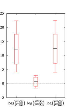
Figure 5: Boxplot of logarithmic Bayes factors computed from 50 independent datasets.

This represents compelling evidence for model 3. The result is not entirely surprising given that this model gives memory to state 2, which is slowly mixing, as indicated in Figure 4. The fact that the most complex model (model 2) is not necessarily selected showcases the automatic penalty for model complexity in Bayes factors.

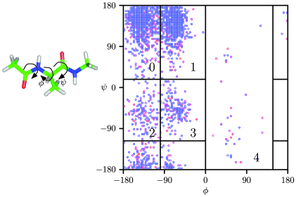
Figure 6: The structure of Ace-Ala-Nme is described by two dihedral angles, $\phi$ and $\psi$. The periodic map on the right shows a partition of conformational space into 5 states. The colored markers indicate the free energy of bins centered at each point, which reveals the metastable nature of this molecule’s dynamics.

We conclude this section with two applications of Bayesian analysis of reversible Markov chains to molecular dynamics (MD). An MD simulation approximates the time-reversible dynamics of a molecule in solvent. The trajectories produced by a simulation are discretized in space and time.

Example 5.6.

The terminally blocked alanine dipeptide, shown in Figure 6, is a common test system for Markov models of MD. The conformational space of the molecule, which is represented in the figure in a two-dimensional projection, is partitioned into 5 states. The states are believed to be metastable due to the basins that characterize the free-energy function, also plotted in the figure. This metastability allows one to approximate the dynamics of the molecule, projected onto the partition, as a reversible Markov chain. The approximation will be good when the discrete time interval at which a trajectory is sampled is larger than the timescale for equilibration within every state, but smaller than the timescale of transitions.

Few statistical validation methods are available for Markov models of MD. Bacallado, Chodera and Pande used a Bayesian hypothesis test to compare different partitions of conformational space Bacallado2009ri . Here, we apply Bayes factors to test a first-order Markov model on a fixed partition, by comparing it to second-order and variable-order models on the same partition. The data $\mathbf{X}$ are the transition counts in a single MD trajectory of 1767 steps sampled at an interval of 6 picoseconds, as recorded in Table 1. The prior parameters $w$ and $\beta$ are the same as in the previous example. The results of the model comparison are summarized in the following table.

Table 1: Molecular dynamics simulation of the alanine dipeptide. The entries in the table are the transition counts $(x_{1},x_{2})\to(x_{2},x_{3})$ in the trajectory $\mathbf{X}$, which has initial state $(0,4)$

		$\bolds{x_{3}}$							$\bolds{x_{3}}$
$\bolds{x_{1}}$	$\bolds{x_{2}}$	0	1	2	3	4	$\bolds{x_{1}}$	$\bolds{x_{2}}$	0	1	2	3	4
0	0	$261$	$187$	$13$	$2$	0	3	0	5	$13$	$2$	0	0
	1	$188$	$144$	$13$	$11$	0		1	5	$4$	$2$	1	0
	2	$12$	$4$	$9$	$15$	0		2	4	$3$	$16$	5	0
	3	$5$	$1$	$0$	$1$	0		3	2	$5$	$3$	3	0
	4	$1$	$0$	$0$	$0$	0		4	0	$0$	$0$	0	0
1	0	$180$	$143$	$22$	$5$	0	4	0	1	$0$	$0$	0	0
	1	$141$	$125$	$5$	$5$	0		1	0	$0$	$0$	0	0
	2	$4$	$3$	$10$	$4$	0		2	0	$0$	$0$	0	0
	3	$4$	$1$	$10$	$3$	0		3	0	$0$	$0$	0	0
	4	$0$	$0$	$0$	$0$	0		4	0	$0$	$0$	0	0
2	0	$16$	$13$	$3$	$0$	0
	1	$16$	$4$	$1$	$1$	0
	2	$12$	$12$	$37$	$11$	0
	3	$9$	$5$	$15$	$6$	0
	4	$0$	$0$	$0$	$0$	0

Model ($\bolds i$)	$\bolds{\log P^{(i)}(\mathbf{X})}$
First order	$-1846$
Variable order 0	$-1824$
Variable order 1	$-1825$
Variable order 2	$-1844$
Variable order 3	$-1846$
Variable order 4	$-1847$
Second order	$\bolds-$1800

The state describing each variable order model is the only state in the model that has a memory of length 2 (the only state that is not a history). There seems to be substantial evidence in favor of a second-order model. Adding memory to states seen in a large number of transition makes a bigger difference, as expected. This result is in accordance with certain exploratory observations which indicate that at the timescale of 6 picoseconds, the effect of water around the molecule, neglected in our state definitions, persists.

Example 5.7.

The alanine pentapeptide is a longer polymer that exhibits a higher degree of structural and dynamical complexity. Buchete and Hummer partition the conformational space of the molecule into 32 states by chemical conventions Buchete2008 . An MD trajectory in conformational space was projected onto this partition, and an exploratory analysis suggested that the effects of memory decay after 500 picoseconds. Accordingly, we take a conformation from the trajectory every 500 picoseconds to form a sequence $\mathbf{X}$ of 1885 steps in $\mathcal{X}=\{0,\ldots,31\}$.

As in previous examples, we tested models with varying lengths of memory. Each model was assigned a conjugate prior, this time setting $w(u)=1/32$ for all $u\in\mathcal{X}^{3}$. Of all the variable-order models where a single state has a memory of length 2 and all others are histories, we found that only 4 models where strongly selected over a first-order model. In the following table, we show the logarithm of the evidence for each of these models, a first-order model and a variable-order model that gives a memory of length 2 to all 4 states.

Model ($\bolds i$)	$\bolds{\log P^{(i)}(\mathbf{X})}$
First order	$-4090.0$
Variable order 14	$-4015.5$
Variable order 15	$-3814.5$
Variable order 30	$-3860.3$
Variable order 31	$-3301.6$
Variable order 14, 15, 30, 31	$\bolds-$2964.3

This represents compelling evidence for a model that gives memory to states 14, 15, 30 and 31. It is interesting to contrast inferences based on this model to those based on a first-order Markov model. To do this, we computed 1000 approximate posterior samples of the transition matrix in each case. This was done by simulating a reinforced random walk, which is a mixture of variable-order Markov chains with the posterior distribution of $T$ as a mixing measure (see Proposition 5.3). The reinforced random walk was simulated $10^{7}$ steps to obtain each sample.

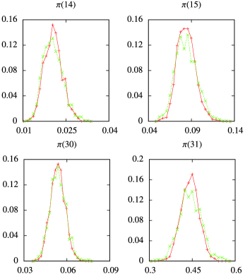
Figure 7: Histograms of 1000 posterior samples of the stationary probabilities of states 14, 15, 30, 31. The red solid lines correspond to the first-order Markov model, and the green dashed lines to the variable-order Markov model that gives a memory of length 2 to states 14, 15, 30 and 31.

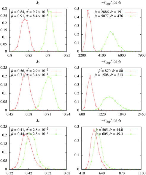
Figure 8: Histograms of 1000 posterior samples of the second, third and fourth largest eigenvalues of the transition matrix, as well as the timescales associated with these eigenvalues. The red solid lines correspond to the first-order Markov model, and the green dashed lines to the variable-order Markov model that gives memory to states 14, 15, 30 and 31. In both cases, we compute the eigenvalues of the transition matrix for the process $V_{n},n\in\mathbb{N}$, in $\mathcal{X}^{2}$. All sample means $\hat{\mu}$ and standard deviations $\hat{\sigma}$ are shown.

In Figure 7, we histogram stationary probabilities of the transition matrices sampled from the posterior. In particular, we show plots for the stationary probabilities of states 14, 15, 30 and 31. In the variable-order model, we define $\pi(x)=\sum_{y\in\mathcal{X}}\pi(xy)$. The inferences of each model in this case are very similar.

The largest eigenvalues of the transition matrix are also of interest because they are related to different modes of relaxation. Each eigenvalue $\lambda$ is associated with a timescale $-\tau_{\mathrm{lag}}/\log\lambda$, which is useful in exploratory analysis. Here, $\tau_{\mathrm{lag}}$ is the length in time of one step of the Markov chain, or 500 picoseconds. In Figure 8, we histogram posterior samples of the three largest nonunit eigenvalues and their associated timescales. In this case, the inferences of each model are quite different, with the variable-order model predicting larger eigenvalues and timescales.

6 Conclusions

We define a reinforcement scheme for the higher-order, reversible Markov chain that extends the ERRW on an undirected graph. Several properties of the ERRW, like recurrence and partial exchangeability, were shown to generalize to this process. Other properties may also generalize but were not pursued here. In particular, we can mention the uniqueness results of Johnson Zabell1982ir and Rolles Rolles2003xd , and the fact that mixtures of measures in $\mathcal{D}$ are weak-star dense in the space of all priors Diaconis2006gd .

The reinforced random walk leads to a conjugate prior that facilitates estimation and hypothesis testing of reversible processes in which the effects of memory decay after some time. Certain statistical problems remain a challenge, such as inferring the transition matrix with a fixed stationary distribution. In applications, it will become important to evaluate the objectivity of the prior and to determine the optimal value of its parameters in this sense.

From a practical point of view, we only discussed Bayesian updating for data sets composed of a single Markov chain starting with probability 1 from the initial state $v_{0}$ used in the prior. Numerical algorithms are needed to perform inference with data sets composed of multiple chains. A starting point could be the method developed by Bacallado, Chodera and Pande to apply the prior of Diaconis and Rolles to first-order, reversible Markov chains Bacallado2009ri .

Appendix

In the following, we use the notation defined in the first paragraph of Section 2.

Proposition .1 ((Kolmogorov’s criterion)).

Let $X_{n},n\in\mathbb{N}$, be an irreducible order-$r$ Markov chain with transition probabilities $p$. Then $X_{n}$ is reversible if and only if for any cyclic admissible path $v_{0},v_{1},\ldots,v_{n},v_{0}$,

$$p(v_{1}|v_{0})p(v_{2}|v_{1})\cdots p(v_{0}|v_{n})=p(v_{0}^{*}|v_{1}^{*})p(v_{1}^{*}|v_{2}^{*})\cdots p(v_{n}^{*}|v_{0}^{*}).$$ (12)

The “only if” statement is straightforward. By the definition of the stationary distribution and reversibility

$$p(v_{1}|v_{0})p(v_{2}|v_{1})\cdots p(v_{0}|v_{n}) = \frac{P_{\pi}(\overline{v_{0}v_{1}})}{\pi(v_{0})}\frac{P_{\pi}(\overline{v_{1}v_{2}})}{\pi(v_{1})}\cdots\frac{P_{\pi}(\overline{v_{n}v_{0}})}{\pi(v_{n})}$$

$$= \frac{P_{\pi}(\overline{v_{1}^{*}v_{0}^{*}})}{\pi(v_{0}^{*})}\frac{P_{\pi}(\overline{v_{2}^{*}v_{1}^{*}})}{\pi(v_{1}^{*})}\cdots\frac{P_{\pi}(\overline{v_{0}^{*}v_{n}^{*}})}{\pi(v_{n}^{*})}$$

$$= p(v_{0}^{*}|v_{1}^{*})p(v_{1}^{*}|v_{2}^{*})\cdots p(v_{n}^{*}|v_{0}^{*}).$$

To prove the “if” statement, choose an arbitrary state $u$; then, for any $v$, since the chain is irreducible, there is an admissible path $u,v_{1},v_{2},\ldots,v_{n},v$ with positive probability. Define

$$\pi^{\prime}(v)=B\frac{p(v_{1}|u)p(v_{2}|v_{1})\cdots p(v|v_{n})}{p(v_{n}^{*}|v^{*})p(v_{n-1}^{*}|v_{n}^{*})\cdots p(u^{*}|v_{1}^{*})},$$ (13)

where $B$ is a positive constant. Note that this expression does not depend on the sequence $v_{1},\ldots,v_{n}$ chosen. Take a different sequence $z_{1},\ldots,z_{m}$. Let $t\in\mathcal{X}^{r}$ be a palindrome, then because the chain is irreducible, we can find a sequence $v,t_{1},t_{2},\ldots,t$ with positive probability, and it is easy to see from equation (12) that the palindrome $v,t_{1},t_{2},\ldots,t,\ldots,t_{2}^{*},t_{1}^{*},v^{*}$ has positive probability. We can construct another palindrome $u^{*},s_{1},s_{2},\ldots,s_{2}^{*},s_{1}^{*},u$ in the same way. Multiplying equation (13) by factors of 1,

$$B\frac{p(v_{1},v_{2},\ldots,v|u)}{p(v_{n}^{*},v_{n-1}^{*},\ldots,u^{*}|v^{*})} = B\frac{p(v_{1},v_{2},\ldots,v|u)}{p(v_{n}^{*},v_{n-1}^{*},\ldots,u^{*}|v^{*})}\frac{p(t_{1},t_{2},\ldots,v^{*}|v)}{p(t_{1},t_{2},\ldots,v^{*}|v)}$$

$${}\times\frac{p(z_{m}^{*},z_{m-1}^{*},\ldots,u^{*}|v^{*})}{p(z_{1},z_{2},\ldots,v|u)}\frac{p(s_{1},s_{2},\ldots,u|u^{*})}{p(s_{1},s_{2},\ldots,u|u^{*})}$$

$${}\times\frac{p(z_{1},z_{2},\ldots,v|u)}{p(z_{m}^{*},z_{m-1}^{*},\ldots,u^{*}|v^{*})}$$

$$= B\frac{p(z_{1},z_{2},\ldots,v|u)}{p(z_{m}^{*},z_{m-1}^{*},\ldots,u^{*}|v^{*})}.$$

The first four terms equal 1 because the numerator and denominator are the probabilities of the same cycle forward and backward, which are equal by equation (12). Now, we check that $\pi^{\prime}(v)$ satisfies the reversibility conditions specified in the Introduction. First, we show that $\pi^{\prime}(v)=\pi^{\prime}(v^{*})$. Take a path $u,z_{1},\ldots,z_{\ell},v^{*}$ with positive probability, and the previously found palindrome $u^{*},s_{1},s_{2},\ldots,s_{2}^{*},s_{1}^{*},u$, then applying the same method,

$$\pi^{\prime}(v) = B\frac{p(v_{1},v_{2},\ldots,v|u)}{p(v_{n}^{*},v_{n-1}^{*},\ldots,u^{*}|v^{*})}$$

$$= B\frac{p(v_{1},v_{2},\ldots,v|u)}{p(v_{n}^{*},v_{n-1}^{*},\ldots,u^{*}|v^{*})}\frac{p(s_{1},s_{2},\ldots,u|u^{*})}{p(s_{1},s_{2},\ldots,u|u^{*})}$$

$${}\times\frac{p(z_{\ell}^{*},z_{\ell-1}^{*},\ldots,u^{*}|v)}{p(z_{1},z_{2},\ldots,v^{*}|u)}\frac{p(z_{1},z_{2},\ldots,v^{*}|u)}{p(z_{\ell}^{*},z_{\ell-1}^{*},\ldots,u^{*}|v)}$$

$$= B\frac{p(z_{1},z_{2},\ldots,v^{*}|u)}{p(z_{\ell}^{*},z_{\ell-1}^{*},\ldots,u^{*}|v)}=\pi^{\prime}(v^{*}).$$

From this, and equation (13) we deduce that for any admissible $v,z$, $\pi^{\prime}(v)p(z|\break v)=\pi^{\prime}(z^{*})p(v^{*}|z^{*})$. Since the state space is finite, we can choose $B$ such that $\pi^{\prime}$ sums to 1. We have shown that the weights $k_{v,z}\equiv\pi^{\prime}(v)p(z|v)$ satisfy the conditions of a reversible random walk with memory, so by Proposition 2.3 the process with transition probabilities $p$ represents a reversible, order-$r$ Markov chain.

Proof of Proposition 4.5 The probability $H_{w,v_{0}}(v_{0},\ldots,v_{m})$ is a product of transition probabilities, to which the $n$th transition contributes a factor of

$$p_{n}=\frac{w^{\prime}_{n-1}(\overline{f(v_{n-1})v_{n}})}{w^{\prime\prime}_{n-1}(f(v_{n-1}))}.$$ (14)

We know that $f(v_{n})$ cannot be longer than $\overline{f(v_{n-1})v_{n}}$ by Proposition 4.2; let $L(v_{n-1},v_{n})$ be the set of histories of $v_{n}$ that are shorter than $f(v_{n-1})$. If this set is nonempty, let us multiply equation (14) by factors of 1, to obtain the following factor for the $n$th transition:

$$p_{n}=\frac{w^{\prime}_{n-1}(\overline{f(v_{n-1})v_{n}})}{w^{\prime\prime}_{n-1}(f(v_{n-1}))}\prod_{z\in L(v_{n-1},v_{n})}\frac{w^{\prime}_{n-1}(z^{+})}{w^{\prime\prime}_{n-1}(z^{+})},$$ (15)

where $z^{+}$ is the ending of $v_{n}$ that is longer than $z$ by 1. The added factor equals 1 because, if $w^{\prime}_{n-1}(z^{+})\neq w^{\prime\prime}_{n-1}(z^{+})$, then $f(v_{n-1})$ must end on $z$, which by definition is a history shorter than $f(v_{n-1})$, a contradiction.

Consider all the possible factors in the numerator of $H_{w,v_{0}}(v_{0},\ldots,v_{m})$. Take any $h\in\mathscr{H}$ that is minimal, meaning that it does not end in another history. For any $a\in\mathcal{X}$, we will see a factor $w^{\prime}(ha)$ after every transition through $ha$. The conjugate factor $w^{\prime}(ah^{*})$ will appear every time we go through $ah^{*}$, because:

• If $\mathrm{A}(ah^{*})\in\mathscr{H}$, it is minimal by the closure properties of $\mathscr{H}$, so $w^{\prime}(ah^{*})$ will be the numerator of the first factor in equation (15).

• Otherwise, the minimal history in the transition ending in $ah^{*}$ will be longer than $h^{*}$, and there will be an added factor in equation (15) with $w^{\prime}(ah^{*})$ in the numerator. Conversely, note that the factor $w^{\prime}(ah^{*})$ is only added to the numerator of equation (15) when we go through $ah^{*}$ for some minimal $h$, because we required that $h^{*}\in L(v_{n-1},v_{n})$, so $h\in\mathscr{H}$ and does not end in another history.

As in the proof of Proposition 3.5, we argue that every new factor $w^{\prime}(ha)$ or $w^{\prime}(ah^{*})$ is increased by $c$ with respect to the previous one (or by $2c$ if $ha$ is a palindrome). Therefore, the numerator of $H_{w,v_{0}}(v_{0},\ldots,v_{m})$ is only a function of the transition counts and the initial state.

Finally, consider all the factors in the denominator of $H_{w,v_{0}}(v_{0},\ldots,v_{m})$. Take any minimal history $h$. We will see a factor $w^{\prime\prime}(h)$, for every transition through $h$. The conjugate factor $w^{\prime\prime}(h^{*})$ will appear every time we go through $h^{*}$, because:

• If $h^{*}$ is also minimal, then $w^{\prime\prime}(h^{*})$ will be in the denominator of the first factor in equation (15).

• Otherwise, we know that $\mathrm{A}(h^{*})$ is not a history, so the transition ending in $h^{*}$ must have a history at least as long as $h^{*}$, which is longer than the history $\Omega(h^{*})$. So, $w^{\prime\prime}(h^{*})$ will appear in the denominator of a factor added in equation (15). Conversely, we only add factors of $w^{\prime\prime}(h^{*})$ to the denominator of equation (15) when we go through $h^{*}$ for a minimal $h$, because we required $\Omega(h^{*})\in L(v_{n-1},v_{n})$ which implies $h$ minimal.

As before, every new factor $w^{\prime\prime}(h)$ or $w^{\prime\prime}(h^{*})$ will be increased by $c$ with respect to the previous one (or by $2c$ if $h$ is a palindrome). Therefore, the denominator is a function of the transition counts and the initial state, and the process is partially exchangeable.

Proof of Proposition 4.6 Let $\vec{C}_{n}(u,v)$ be the transition counts from $u$ to $v$ in the first $n$ steps of a stochastic process on $\mathcal{X}^{r}$. Also, define $\vec{C}_{n}(u)\equiv\sum_{v\in\mathcal{X}^{r}}\vec{C}_{n}(u,v)$, which counts the visits to $u$. Remember $\mathcal{T}^{\prime\prime}$ is the set of irreducible transition matrices for variable-order, reversible Markov chains where all $h\in\mathscr{H}$ are histories. Define the event $D$, that the set $\{\vec{C}_{n}(u,v)/\vec{C}_{n}(u)\dvtx\forall u,v$ admissible$\}$ converges to a transition probability matrix in $\mathcal{T}^{\prime\prime}$.

From the recurrence of the variable-order, reinforced random walk and equation (7), it is evident that the set of irreducible Markov chains has measure 1 under $\psi_{w,v_{0}}$. In this set, the variables $\{\vec{C}_{n}(u,v)/\vec{C}_{n}(u)\dvtx\forall u,v\mbox{ admissible}\}$ converge almost surely to the transition probabilities, so for any $T\notin\mathcal{T}^{\prime\prime}$ irreducible, $P_{v_{0}}^{T}(D)=0$. Furthermore, by Lemma .3, $D$ happens almost surely in the variable-order, reinforced random walk. Putting this into equation (7), we have

$$H_{w,v_{0}}(D)=1=\int_{\mathcal{T}}P_{v_{0}}^{T}(D)\,d\psi_{w,v_{0}}(T)\leq\int_{\mathcal{T}^{\prime\prime}}\,d\psi_{w,v_{0}}(T),$$

which implies the proposition.

Lemma .2 ((Lévy)).

Consider a sequence of events $B_{k}\in\mathcal{F}_{k},k\in\mathbb{N}$, in some filtration $\{\mathcal{F}_{k}\}$. Let $b_{n}=\sum_{k=1}^{n}\mathbf{1}_{B_{n}}$ be the total number of events occurring among the first $n$, and let $s_{n}=\sum_{k=1}^{n}P(B_{k}|\mathcal{F}_{k-1})$ be the sum of the first $n$ conditional probabilities. Then, for almost every $\omega$:

• If $s_{n}(\omega)$ converges as $n\to\infty$, then $b_{n}(\omega)$ has a finite limit.

• If $s_{n}(\omega)$ diverges, then $b_{n}(\omega)/s_{n}(\omega)\to 1$.

Lemma .3.

$H_{w,v_{0}}(D)=1$.

For any $u$ in $\{\mathcal{X}^{q}\dvtx q\leq r+1\}$, the variables $n^{-1}w^{\prime}_{n}(u)$ and$n^{-1}w^{\prime\prime}_{n}(u)$ are functions of $\{n^{-1}\vec{C}_{n}(u,v)\dvtx\forall u,v\mbox{ admissible}\}$, therefore they converge almost surely, because the reinforced random walk is a mixture of irreducible Markov chains for which the latter converge. The reinforcement scheme defined in Definition 4.3 imposes some constraints on the limits of $n^{-1}w^{\prime}_{n}(u)$ and $n^{-1}w^{\prime\prime}_{n}(u)$. Note that $w^{\prime\prime}_{n}(u)$, $w^{\prime\prime}_{n}(u^{*})$, $w^{\prime}_{n}(u)$ and $w^{\prime}_{n}(u^{*})$ never differ by more than $c$; we also know that the reinforced random walk is positive recurrent (it is a mixture of irreducible, finitely-valued Markov chains), so almost surely

$$\lim_{n\to\infty}n^{-1}w^{\prime\prime}_{n}(u) = \lim_{n\to\infty}n^{-1}w^{\prime\prime}_{n}(u^{*})=\lim_{n\to\infty}n^{-1}w^{\prime}_{n}(u)$$

$$= \lim_{n\to\infty}n^{-1}w^{\prime}_{n}(u^{*})>0.$$

Denote this limit $w_{\infty}(u)=w_{\infty}(u^{*})$. It is also easy to see that if $u\in\mathcal{X}^{q}$, then for all $s>q$,

$$\sum_{\{v\in\mathcal{X}^{s}\dvtx v\mathrm{\ ends\ in\ }u\}}w_{\infty}(v)=w_{\infty}(u).$$ (17)

Now, let $\tau_{n}$ be the $n$th visit to $u\in\mathcal{X}^{r}$ and let $B_{n}$ be the event that we make a transition to $v$ at $\tau_{n}$. Define

$$p_{n}(f(u),v)\equiv H_{w,v_{0}}(B_{n}|\sigma(Y_{1},\ldots,Y_{\tau_{n}}))=\frac{w^{\prime}_{\tau_{n}}(\overline{f(u)v})}{w^{\prime\prime}_{\tau_{n}}(f(u))}.$$

We know $p_{n}(f(u),v)$ converges a.s. to $w_{\infty}(\overline{f(u)v})/w_{\infty}(f(u))>0$. Therefore, $\sum_{n}p_{n}(f(u),v)=\infty$ a.s., and by Lévy’s extension of the Borel–Cantelli lemma (Lemma .2),

$$\frac{\sum_{m=1}^{n}\mathbf{1}_{B_{m}}}{\sum_{m=1}^{n}p_{m}(f(u),v)}\to 1\quad\mbox{a.s.}$$

$$\qquad\Longrightarrow\quad\lim_{n\to\infty}\frac{1}{n}\sum_{m=1}^{n}\mathbf{1}_{B_{m}}=\lim_{k\to\infty}\frac{\vec{C}_{k}(u,v)}{\vec{C}_{k}(u)}=\frac{w_{\infty}(\overline{f(u)v})}{w_{\infty}(f(u))}.$$

This means that $\{\vec{C}_{n}(u,v)/\vec{C}_{n}(u)\dvtx\forall u,v\mbox{ admissible}\}$ converges $H_{w,v_{0}}$-a.s. to a set of transition probabilities, $w_{\infty}(\overline{f(u)v})/w_{\infty}(f(u))$, for a variable-order Markov chain with histories $\mathscr{H}$. To show that this Markov chain is reversible, note that $w_{\infty}$ is the stationary distribution, because

$$\sum_{{{{\left\{\matrix{u\in\mathcal{X}^{r}{:}\cr u,v\mathrm{\ admissible}}\right\}}}}}w_{\infty}(u)\frac{w_{\infty}(\overline{f(u)v})}{w_{\infty}(f(u))} = \sum_{{{\left\{\matrix{h\in\mathscr{H}\mathrm{\ minimal{:}}\cr h,v\mathrm{\ admissible}}\right\}}}}\sum_{\{u\dvtx f(u)=h\}}w_{\infty}(u)\frac{w_{\infty}(\overline{hv})}{w_{\infty}(h)}$$

$$= \sum_{{{\left\{\matrix{h\in\mathscr{H}\mathrm{\ minimal{:}}\cr h,v\mathrm{\ admissible}}\right\}}}}w_{\infty}(h)\frac{w_{\infty}(\overline{hv})}{w_{\infty}(h)}$$

$$= w_{\infty}(v),$$

where we used equation (17) in the last two identities. By equation (Appendix), $w_{\infty}$ satisfies the conditions for reversibility. Therefore, $H_{w,v_{0}}(D)=1$.

References

- (1) {bunpublished}[author] \bauthor\bsnmAldous, \bfnmD.\binitsD. and \bauthor\bsnmFill, \bfnmJ.\binitsJ. \btitleReversible Markov chains and random walks on graphs. \bnoteUnpublished manuscript. \endbibitem
- (2) {bmisc}[author] \bauthor\bsnmBacallado, \bfnmS.\binitsS. (\byear2010). \btitleSupplement to “Bayesian analysis of variable-order, reversible Markov chains.” DOI:10.1214/10-AOS857SUPP. \endbibitem
- (3) {barticle}[author] \bauthor\bsnmBacallado, \bfnmSergio\binitsS., \bauthor\bsnmChodera, \bfnmJohn D.\binitsJ. D. and \bauthor\bsnmPande, \bfnmVijay\binitsV. (\byear2009). \btitleBayesian comparison of Markov models of molecular dynamics with detailed balance constraint. \bjournalJ. Chem. Phys. \bvolume131 \bpages045106. \endbibitem
- (4) {barticle}[author] \bauthor\bsnmBegleiter, \bfnmR.\binitsR., \bauthor\bsnmEl-Yaniv, \bfnmR.\binitsR. and \bauthor\bsnmYona, \bfnmG.\binitsG. (\byear2004). \btitleOn prediction using variable order Markov models. \bjournalJ. Artificial Intelligence Res. \bvolume22 \bpages385–421. \MR2129473 \endbibitem
- (5) {barticle}[author] \bauthor\bsnmBuchete, \bfnmN.V.\binitsN. and \bauthor\bsnmHummer, \bfnmG.\binitsG. (\byear2008). \btitleCoarse master equations for peptide folding dynamics. \bjournalJ. Phys. Chem. B \bvolume112 \bpages6057–6069. \endbibitem
- (6) {barticle}[author] \bauthor\bsnmBühlmann, \bfnmP.\binitsP. (\byear2000). \btitleModel selection for variable length Markov chains and tuning the context algorithm. \bjournalAnn. Inst. Statist. Math. \bvolume52 \bpages287–315. \MR1763564 \endbibitem
- (7) {barticle}[author] \bauthor\bsnmBühlmann, \bfnmPeter\binitsP. and \bauthor\bsnmWyner, \bfnmAbraham J.\binitsA. J. (\byear1999). \btitleVariable length Markov chains. \bjournalAnn. Statist. \bvolume27 \bpages480–513. \MR1714720 \endbibitem
- (8) {barticle}[author] \bauthor\bsnmDiaconis, \bfnmP\binitsP. and \bauthor\bsnmFreedman, \bfnmD\binitsD. (\byear1980). \btitlede Finetti theorem for Markov chains. \bjournalAnn. Probab. \bvolume8 \bpages115–130. \MR0556418 \endbibitem
- (9) {binproceedings}[author] \bauthor\bsnmDiaconis, \bfnmPersi\binitsP. (\byear1988). \btitleRecent progress on de Finetti notions of exchangeability. In \bbooktitleBayesian Statistics 3 (\beditor\bfnmJ. M.\binitsJ. M. \bsnmBernardo, \beditor\bfnmM. H.\binitsM. H. \bsnmDeGroot, \beditor\bfnmD. V.\binitsD. V. \bsnmLindley and \beditor\bfnmA. F. M\binitsA. F. M. \bsnmSmith, eds.) \bpages111–125. \bpublisherOxford Univ. Press, \baddressNew York. \MR1008047 \endbibitem
- (10) {barticle}[author] \bauthor\bsnmDiaconis, \bfnmPersi\binitsP. and \bauthor\bsnmRolles, \bfnmSilke\binitsS. (\byear2006). \btitleBayesian analysis for reversible Markov chains. \bjournalAnn. Statist. \bvolume34 \bpages1270–1292. \MR2278358 \endbibitem
- (11) {barticle}[author] \bauthor\bsnmKass, \bfnmR\binitsR. and \bauthor\bsnmRaftery, \bfnmA\binitsA. (\byear1995). \btitleBayes factors. \bjournalJ. Amer. Statist. Assoc. \bvolume90 \bpages773–795. \endbibitem
- (12) {bincollection}[author] \bauthor\bsnmKeane, \bfnmMS\binitsM. and \bauthor\bsnmRolles, \bfnmSilke\binitsS. (\byear2000). \btitleEdge-reinforced random walk on finite graphs. In \bbooktitleInfinite Dimensional Stochastic Analysis \bpages217–234. \bpublisherR. Neth. Acad. Arts Sci., \baddressAmsterdam. \MR1832379 \endbibitem
- (13) {bbook}[author] \bauthor\bsnmKelly, \bfnmF. P\binitsF. P. (\byear1979). \btitleReversibility and Stochastic Networks. \bpublisherWiley, \baddressChichester. \MR0554920 \endbibitem
- (14) {barticle}[author] \bauthor\bsnmMacQueen, \bfnmJ\binitsJ. (\byear1981). \btitleCircuit processes. \bjournalAnn. Probab. \bvolume9 \bpages604–610. \MR0624686 \endbibitem
- (15) {barticle}[author] \bauthor\bsnmRissanen, \bfnmJ.\binitsJ. (\byear1983). \btitleA universal data compression system. \bjournalIEEE Trans. Inform. Theory \bvolume29 \bpages656–664. \MR0730903 \endbibitem
- (16) {barticle}[author] \bauthor\bsnmRolles, \bfnmSilke\binitsS. (\byear2003). \btitleHow edge-reinforced random walk arises naturally. \bjournalProbab. Theory Related Fields \bvolume126 \bpages243–260. \MR1990056 \endbibitem
- (17) {barticle}[author] \bauthor\bsnmWeinberger, \bfnmM.J.\binitsM., \bauthor\bsnmRissanen, \bfnmJ.J.\binitsJ. and \bauthor\bsnmFeder, \bfnmM.\binitsM. (\byear1995). \btitleA universal finite memory source. \bjournalIEEE Trans. Inform. Theory \bvolume41 \bpages643–652. \endbibitem
- (18) {barticle}[author] \bauthor\bsnmZabell, \bfnmSL\binitsS. (\byear1982). \btitleW. E. Johnson’s sufficientness postulate. \bjournalAnn. Statist. \bvolume10 \bpages1091–1099. \MR0673645 \endbibitem