Hubble Space Telescope Observations of Field Ultracool Dwarfs at High Galactic Latitude

Abstract

We present a sample of 17 newly discovered ultracool dwarf candidates later than $\sim\!\mathrm{M}8$, drawn from 231.90 arcmin² of Hubble Space Telescope Wide Field Camera 3 infrared imaging. By comparing the observed number counts for $17.5\!\leq\!J_{125}\!\leq\!25.5$ AB mag to an exponential disk model, we estimate a vertical scale height of $z_{scl}\!=\!290\pm 25\;(\mathrm{random})\pm 31\;(\mathrm{systematic})$ pc for a binarity fraction of $f_{b}\!=\!0$. While our estimate is roughly consistent with published results, we suggest that the differences can be attributed to sample properties, with the present sample containing far more substellar objects than previous work. We predict the object counts should peak at $J_{125}\!\sim\!24$ AB mag due to the exponentially-declining number density at the edge of the disc. We conclude by arguing that trend in scale height with spectral type may breakdown for brown dwarfs since they do not settle onto the main sequence.

1. Introduction

Star counts have long been used to determine the structure of our Galaxy. Early attempts were plagued by patchy extinction and by mathematical instabilities in the inversion of star counts (see Bok, 1937), but Bahcall & Soneira (1980, 1984) revived the endeavor by avoiding regions with significant extinction, and by fitting a physically motivated model with only a few parameters (see Bahcall 1986 for a review). Recently, there has been renewed interest in star counts as ever-cooler stellar populations are discovered and need to be modeled (Ryan et al., 2005; Pirzkal et al., 2005; Caballero, Burgasser, & Klement, 2008; Jurić et al., 2008; Pirzkal et al., 2009; Deacon et al., 2009; Bochanski et al., 2010; Delorme et al., 2010). Because brown dwarfs cool and change spectral type on relatively short timescales, their vertical scale heights may reflect not just Galactic structure, but also their cooling times.

The Galactic distribution of the ultracool dwarf population has garnered much interest from a community studying far more distant objects. Since the extremely red optical and near-infrared colors of the ultracool dwarfs are similar to those of Lyman-break galaxies (LBGs; Steidel et al., 1996) at redshifts of $5\!\lesssim\!z\!\lesssim\!7$, there are concerns that the high-redshift galaxy samples may be contaminated by these Galactic objects (e.g. Caballero, Burgasser, & Klement, 2008). In the absence of spectroscopic identification, LBG studies often resort to statistically correcting their number counts for foreground contamination (e.g. Bouwens et al., 2006). Naturally, this correction relies on accurately characterizing the Galactic distribution of ultracool dwarfs. To this end, Ryan et al. (2005) identify 28 dwarfs with $(i^{\prime}-z^{\prime})_{\rm AB}\!\geq\!1.3$ mag (which are types later than $\sim\!\mathrm{M}6$; Bochanski et al., 2010) in 15 parallel fields from the Advanced Camera for Surveys (ACS) aboard the Hubble Space Telescope (HST). By assuming an exponential disk model, Ryan et al. (2005) derive a vertical scale height of $z_{scl}\!=\!350\pm 50$ pc, and conclude that the deepest surveys of $z\!\simeq\!6$ LBGs were $\gtrsim\!97$% pure. Similarly, Pirzkal et al. (2005) find a vertical scale height of $z_{scl}\!=\!400\pm 100$ pc from three spectroscopically identified late-M and early-L dwarfs in the Hubble Ultra Deep Field (Beckwith et al., 2006).

The overwhelming majority of ultracool dwarfs to date have been found in shallow, very wide-field surveys (e.g. Delfosse et al., 1999; Kirkpatrick et al., 1999; Knapp et al., 2004), and more recently with deeper datasets (e.g. Delorme et al., 2008; Deacon et al., 2009). Since these objects are intrinsically very faint ($M_{i^{\prime}}\!\gtrsim\!16$ mag; Hawley et al., 2002), nearly all known ultracool dwarfs reside within $\sim\!100$ pc of the Sun (e.g. Reid et al., 2008), which makes determining the Galactic-scale distribution difficult or impossible. While this issue can be mitigated to a large extent by probing further into the disk, limited observing time and detection efficiency have restricted studies to narrow fields-of-view and/or single lines-of-sight (e.g. Ryan et al., 2005; Pirzkal et al., 2005, 2009). Naturally this leads to simplified models, large uncertainties on model parameters, and significant variations between authors. In this paper, we begin to overcome these limitations by drawing our sample from very deep parallel and pointed fields with HST, which have the sensitivity to find an L0-dwarf to $\sim\!3.5$ kpc and a T0-dwarf to $\sim\!700$ pc. These represent a significant increase in survey distances for ultracool dwarfs.

This work is organized as follows: in § 2 we describe the observations and source catalogs, in § 3 we discuss our ultracool dwarf sample selection, in § 4 we present our analysis and scale height measurement, in § 5 we assess our systematic uncertainties, and in § 6 we conclude with a brief review and thoughts toward future improvements. Unless explicitly stated otherwise, all magnitudes and colors are given in the AB system (Oke & Gunn, 1983).

2. Observations

Here we discuss the parallel and pointed fields with HST which consititute our dataset. We list their salient properties in Table 1.

2.1. The HST Parallel Imaging

The bulk of the data analyzed here come from the high-level science products from the Hubble Infrared Pure Parallel Imaging Extragalactic Survey (HIPPIES; Yan et al., 2011). At present, this survey combines two pure parallel imaging programs with HST  Wide Field Camera 3 (WFC3; PropIDs: 11700 and 11702) and coordinated parallels from the Cosmic Origins Spectrograph (COS) guaranteed time observations (GTO). Every field has infrared imaging in F098M, F125W, and F160W, and optical imaging in F606W and/or F600LP. By design, these fields are at relatively high Galactic latitude ($|b|\!>\!20^{\circ}$), have a total exposure time of $\geq\!4$ HST  orbits, and sample random pointings through the Galaxy.

The data reduction and mosaicking of the HIPPIES data are discussed in detail by Yan et al. (2011), but we will mention the key steps relevant for this work. Standard procedures were followed except for enhanced removal of image defects. Since the HST parallel data are rarely dithered, the affected pixels were corrected by interpolating over neighboring pixels with the FIXPIX routine in IRAF. The main side-effect of this procedure is to decrease the usable area of each parallel pointing. In total, we analyzed 39 parallel fields which cover 185.41 arcmin². Finally, we note that the COS GTO parallel fields also have additional imaging in F300X, F475W, and F475X, though we place no constraints on the colors in these bands.

2.2. The WFC3 Early Release Science Program

In addition to the parallel data, we include the WFC3 Early Release Science program (ERS; PropID: 11359) data taken in the southern field of the Great Observatories Origins Deep Survey (GOODS-S; Giavalisco et al., 2004). The WFC3 imaging in the F098M, F125W, and F160W-bands augments the existing optical data from the ACS and covers $46.49$ arcmin². The ERS data have at least double the exposure time of the WFC3 parallel data in all bands. Details of the ERS data, such as experimental design, reduction, and imaging properties are discussed by Windhorst et al. (2011). Like the COS GTO parallels, the ERS subset of the GOODS-S field has been observed in many additional optical and ultraviolet bands, however we will not impose constraints on those colors to ensure a uniformly selected sample.

Table 1Survey Fields

Field	RA†	Dec†	$\ell^{\dagger}$	$b^{\dagger}$	$\Delta\Omega^{\ddagger}$	$J_{50}^{*}$	$A_{J}^{**}$	Optical
	(${}^{\rm h}\;{}^{\rm m}\;{}^{\rm s}$)	(${}^{\circ}\;{}^{\prime}\;"$)	(deg)	(deg)	($\square^{\prime}$)	(mag)	(mag)	Band
par0110$-$0222	$01\;10\;09.45$	$-02\;22\;23.0$	133.987232	$-64.842182$	4.68	27.69	0.04	BOTH
par0213$+$1254	$02\;13\;38.75$	$+12\;54\;59.2$	152.018742	$-45.261886$	4.69	27.02	0.11	F600LP
cos0227$-$4101	$02\;27\;56.91$	$-41\;01\;34.4$	254.161369	$-65.792729$	4.69	28.00	0.01	F600LP
cos0240$-$1857	$02\;40\;27.63$	$-18\;57\;14.4$	200.649009	$-63.686780$	4.69	27.95	0.03	F600LP
ERS	$03\;32\;23.03$	$-27\;42\;50.2$	223.407959	$-54.441403$	46.49	28.20	0.01	F606W
cos0439$-$5316	$04\;39\;25.42$	$-53\;16\;40.4$	261.334943	$-40.946276$	4.69	28.21	0.00	F600LP
par0539$-$6409	$05\;39\;30.82$	$-64\;09\;03.4$	273.650747	$-32.015470$	4.72	26.45	0.05	F606W
par0553$-$6405	$05\;53\;06.02$	$-64\;05\;18.0$	273.525663	$-30.535557$	4.76	27.01	0.04	F606W
par0623$-$6431	$06\;23\;34.06$	$-64\;31\;49.1$	274.232994	$-27.264246$	4.68	26.32	0.05	F606W
par0623$-$6439	$06\;23\;48.13$	$-64\;39\;41.0$	274.382687	$-27.253780$	4.71	26.94	0.05	F606W
par0637$-$7519	$06\;37\;05.02$	$-75\;18\;39.4$	286.419000	$-27.078161$	6.92	26.98	0.09	F606W
par0750$+$2917	$07\;50\;50.58$	$+29\;16\;53.6$	191.358334	$+24.960307$	4.81	27.43	0.04	BOTH
par0755$+$3043	$07\;55\;57.08$	$+30\;43\;10.9$	190.214896	$+26.453597$	4.68	26.71	0.06	F606W
par0808$+$3945	$08\;08\;21.38$	$+39\;45\;25.3$	180.923544	$+31.128501$	4.68	25.49	0.04	F606W
par0819$+$4911	$08\;19\;19.04$	$+49\;11\;05.4$	170.093673	$+34.244836$	4.68	27.72	0.05	F606W
par0820$+$2332	$08\;20\;03.41$	$+23\;32\;05.0$	199.823952	$+29.326292$	4.69	27.29	0.04	F606W
cos0846$+$7653	$08\;46\;22.36$	$+76\;53\;39.8$	136.607977	$+32.760135$	4.68	28.35	0.02	F600LP
par0905$+$0255	$09\;05\;37.52$	$+02\;55\;31.6$	226.848178	$+30.961043$	4.68	27.03	0.03	F606W
par0909$-$0001	$09\;09\;09.14$	$-00\;01\;47.1$	230.318031	$+30.194936$	4.68	27.36	0.03	F606W
par0914$+$2821	$09\;14\;16.82$	$+28\;21\;44.6$	198.147026	$+42.355984$	4.68	27.50	0.02	F606W
par0921$+$4505	$09\;21\;38.15$	$+45\;05\;08.0$	175.142310	$+44.900120$	4.68	27.16	0.02	F606W
par0925$+$4425	$09\;25\;32.15$	$+44\;25\;31.8$	175.989494	$+45.648179$	4.69	27.85	0.01	F600LP
par0925$+$4000	$09\;25\;35.45$	$+40\;00\;13.0$	182.321062	$+45.878836$	4.68	27.49	0.01	F606W
par1030$+$3803	$10\;30\;52.52$	$+38\;03\;24.5$	183.565827	$+58.665121$	4.68	27.62	0.01	F606W
cos1131$+$3117	$11\;31\;29.93$	$+31\;17\;21.8$	194.732083	$+72.094827$	4.69	27.98	0.02	F600LP
par1151$+$5441	$11\;51\;49.26$	$+54\;40\;59.8$	140.435934	$+60.372625$	4.71	27.70	0.01	F606W
par1152$+$0056	$11\;52\;43.92$	$+00\;55\;51.2$	272.228218	$+60.255125$	4.68	27.78	0.02	F606W
par1209$+$4543	$12\;09\;24.82$	$+45\;43\;26.1$	144.367666	$+69.615667$	4.70	28.09	0.01	BOTH
par1244$+$3356	$12\;44\;45.21$	$+33\;56\;05.1$	134.455667	$+83.043441$	4.68	28.13	0.01	F606W
par1301$-$0000	$13\;01\;16.61$	$-00\;00\;27.0$	308.312235	$+62.761347$	4.68	27.38	0.02	F600LP
par1336$-$0027	$13\;36\;48.75$	$-00\;27\;57.9$	326.341678	$+60.326874$	4.68	27.86	0.03	F600LP
par1340$+$4123	$13\;40\;31.87$	$+41\;23\;03.3$	90.813506	$+72.543346$	4.68	28.17	0.01	F600LP
par1436$+$5043	$14\;36\;56.72$	$+50\;42\;58.6$	89.753150	$+59.068438$	4.69	28.19	0.01	F606W
par1524$+$0954	$15\;24\;10.17$	$+09\;54\;19.8$	14.751734	$+50.137021$	4.68	27.64	0.04	F600LP
par1631$+$3736	$16\;31\;34.28$	$+37\;36\;21.4$	60.300146	$+43.026120$	4.68	27.83	0.01	F606W
par1632$+$3733	$16\;32\;18.38$	$+37\;33\;24.3$	60.246932	$+42.877428$	4.68	27.64	0.01	F606W
cos2057$-$4412	$20\;57\;22.01$	$-44\;12\;26.9$	356.582832	$-40.624781$	4.68	27.45	0.03	F600LP
cos2202$+$1851	$22\;02\;48.68$	$+18\;50\;58.5$	76.653695	$-28.493144$	4.92	28.10	0.06	F600LP
par2345$-$0054	$23\;45\;02.34$	$-00\;54\;11.0$	88.894697	$-59.313985$	4.68	27.83	0.03	F600LP
cos2350$-$4331	$23\;50\;36.39$	$-43\;31\;30.3$	335.844576	$-69.509649$	4.68	28.18	0.01	F600LP
†Coordinates refer to the field center in the J2000 epoch.
‡Solid angle in arcmin2.
∗The approximate 50% completeness limit.
∗∗The $J$-band extinction from Schlegel, Finkbeiner, & Davis (1998).

2.3. Photometry

We measure all magnitudes as MAG_AUTO with SExtractor  (Bertin & Arnouts, 1996) in dual-image mode using the F125W image for detection. We require a minimum area of 5 connected pixels, a threshold (per pixel) of $\geq\!1.5~{}\sigma$ over the local background, and use a $5\times 5$ pix Gaussian filter with full width at half maximum of $2$ pix for source detection. All images are drizzled to $0\farcs 090$ pix^-1. We use 64 deblending sub-thresholds, a minimum contrast parameter of $10^{-4}$, and a cleaning efficiency of 10. We adopt the AB zeropoints from Kalirai et al. (2009a, b) for the WFC3 data of $\mathrm{F606W}\!=\!26.08$ mag, $\mathrm{F600LP}\!=\!25.85$ mag, $\mathrm{F098M}\!=\!25.68$ mag, $\mathrm{F125W}\!=\!26.27$ mag, and $\mathrm{F160W}\!=\!25.96$ mag, and $\mathrm{F606W}\!=\!26.486$ mag for the ACS data in the GOODS-S field. Based on these object catalogs, we compute the 50% completeness depth in the F125W image as the magnitude where the ratio of the observed counts to a power-law fit falls to 0.5, and report these depths in Table 1.

The parallel and ERS data give us a total of $40$ independent sight lines through the disk which cover a total of $231.90$ arcmin². As mentioned above, each field has the same three near-infrared bands; however, the optical imaging differs in wavelength and instrument. In 1, we show our optical and infrared bandpasses: F606W (solid blue), F600LP (dashed blue), F098M (cyan), F125W (green), and F160W (red), which we refer to as $V_{606}$, $I_{600}$, $Y_{098}$, $J_{125}$, and $H_{160}$, respectively.

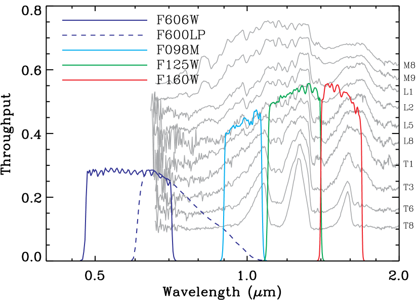
Figure 1.— HST/WFC3 filter throughput curves. The five filters used here are shown as F606W ($V_{606}$; solid blue), F600LP ($I_{600}$; dotted blue), F098M ($Y_{098}$; solid cyan), F125W ($J_{125}$; solid green), and F160W ($H_{160}$; solid red). In light gray lines, we show select spectra from the A. Burgasser SpeX compilation (see Table 2) with infrared types indicated on the left. The COS coordinated parallels and the ERS field have additional blue filters from HST. However, we do not explicitly place constraints on these colors, in order to ensure a uniform sample.

Table 2SpeX Catalog^†

Reference	Number of
	Citations
A. Burgasser (unpublished)	389
Burgasser et al. (2010)	116
Burgasser et al. (2004a)	87
Chiu et al. (2006)	51
Burgasser et al. (2008a)	45
Burgasser et al. (2006a)	19
Muench et al. (2007)	17
Looper, Kirkpatrick, & Burgasser (2007a)	14
Burgasser, Burrows, & Kirkpatrick (2006b)	12
Burgasser (2007a)	8
Siegler et al. (2007)	7
Burgasser et al. (2007b)	6
Burgasser & McElwain (2006)	6
Sheppard & Cushing (2009)	6
Cruz et al. (2004)	5
Burgasser & Kirkpatrick (2006)	4
Looper et al. (2008)	3
Burgasser et al. (2004b)	3
Looper et al. (2007b)	3
McElwain & Burgasser (2006)	3
Reid et al. (2006)	3
Muno et al. (2006)	2
Burgasser et al. (2008b)	2
Burgasser et al. (2009)	1
Luhman et al. (2007)	1
Kirkpatrick et al. (2006)	1
Burgasser (2007c)	1
Burgasser (2007d)	1
Liebert & Burgasser (2007)	1
†Compiled A. Burgasser and distributed at
http://web.mit.edu/ajb/www/browndwarfs/spexprism/

3. Ultracool Dwarf Candidates

3.1. Sample Selection

To ensure that our objects are point-like, we require the axis ratio to be $(b/a)\!\geq\!0.7$ and the half-light radius as measured by FLUX_RADIUS in SExtractor to be $1.2\!\leq\!r_{50}\!\leq\!1.8$ pix. While unsaturated point-sources should have half-light radii roughly independent of brightness, we find a weak trend in the stellar locus, therefore our exact half-light radii limits vary slightly with magnitude. Using the morphological criteria presented in 2, we identify 5982 point sources in the 231.90 arcmin² surveyed.

Figure 2.— Morphological selection criteria. We use the half-light radius, axis ratio, and brightness as measured by SExtractor to identify point sources. The small dots represent all objects from the 231.90 arcmin² analyzed here, and the solid lines show the stellar locus selection region. We find a very weak relationship between half-light radius and brightness. Our constraints on half-light radius and axis ratio are consistent with known stars selected from the Sloan Digital Sky Survey.

We select our ultracool dwarf candidates from the catalog of point sources based on their optical and near-infrared colors. We synthesize empirical $(V_{606}-Y_{098})$, $(I_{600}-Y_{098})$, $(Y_{098}-J_{125})$, and $(J_{125}-H_{160})$ colors from a library of spectra from the 3-meter NASA Infrared Telescope Facility compiled by A. Burgasser (listed in Table 2). In 3, we show the infrared color–color diagram for known L-dwarfs (green triangles), T-dwarfs (red circles), and M-dwarfs, giants, and subdwarfs (blue, magenta, and cyan squares, respectively). Unfortunately, our broadband data cannot accurately constrain the spectral type since the $J_{125}$- and $H_{160}$-bands equally sample the strong H₂O absorption at $\lambda\!=\!1.34~{}\mu$m (see 1). Therefore, the only unique spectral types we can derive from these near-infrared data are given by

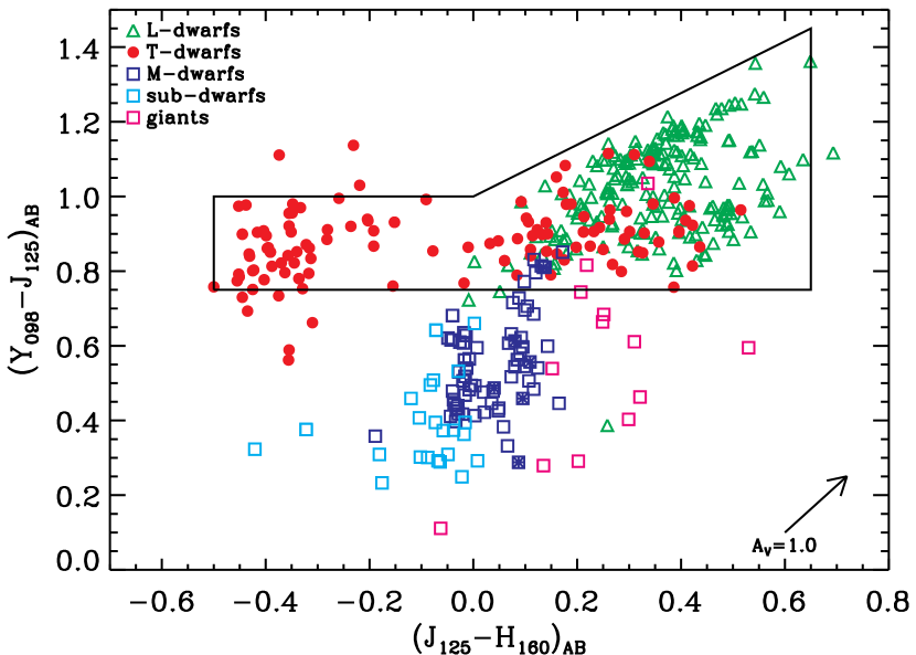
Figure 3.— Color–color diagram for ultracool dwarf selection. We show library of empirical L- and T-dwarfs from the SpeX spectrograph compiled by A. Burgasser (see Table 2) as green triangles and red circles, respectively. We show the M-dwarfs, giants, and subdwarfs as blue, magenta, and cyan squares, respectively. Based on these colors, we define unique spectral types as equations (3), (6), and (9).

$$\mathrm{MLT}\left\{\begin{array}[]{ll}0.0\leq(J_{125}-H_{160})\leq 0.65\>\hbox{mag; and}\\ 0.75\leq(Y_{098}-J_{125})\leq 1.0\>\hbox{mag}\end{array}\right.$$ (3)

$$\mathrm{L}\left\{\begin{array}[]{ll}0.0\leq(J_{125}-H_{160})\leq 0.65\>\hbox{mag; and}\\ 1.0\leq(Y_{098}-J_{160})\leq 0.7\times(J_{125}-H_{160})+1.0\>\hbox{mag}\end{array}\right.$$ (6)

$$\mathrm{T}\left\{\begin{array}[]{ll}-0.5\leq(J_{125}-H_{160})\leq 0.0\>\hbox{mag; and}\\ 0.75\leq(Y_{125}-J_{160})\leq 1.0\>\hbox{mag}\end{array}\right.$$ (9)

For all types, we require $(V_{606}-Y_{098})\!\geq\!2.0$ mag and/or $(I_{600}-Y_{098})\!\geq\!0.5$ mag. We present our ultracool dwarf candidates in Table 3.

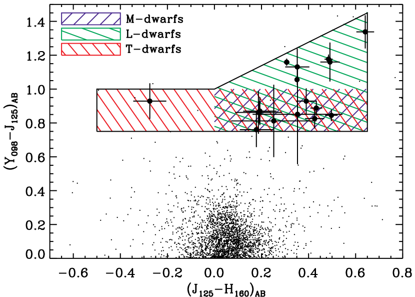
Figure 4.— Color–color diagram for ultracool dwarf candidates. We show the selection region defined by equations (3), (6), and (9) as thick lines and all objects passing our brightness and morphological criteria as small points. In blue, green, and red hatches, we show the expected colors of M-, L-, and T-dwarfs to highlight the ambiguity in spectral typing these stars with these bandpasses. The points with uncertainties represent our 17 ultracool dwarf candidates in Table 3.

3.2. Contaminants

In addition to the ultracool dwarfs, there are three additional types of known astrophysical objects which may satisfy our optical and near-infrared color criteria: early-type galaxies (ETGs), LBGs, and high redshift quasars. In the absence of spectroscopic confirmation, we can only make statistical arguments on these potential objects:

Based on the Coleman, Wu, & Weedman (1980) spectral templates, we estimate that an ETG at $1.2\lesssim\!z\!\lesssim\!1.5$ will have optical and infrared colors similar to our ultracool dwarfs. By extrapolating the luminosity function of ETGs at $z\!=\!1$ (Faber et al., 2007), we find that our fields could have $\sim\!80$ ETGs at these redshifts. However, the number of ETG contaminants in our sample should be much lower, since we require our stellar candidates be unresolved, which is not represented in this simple brightness calculation. To estimate the fraction of these ETGs that are also unresolved, we perform a simple Monte Carlo simulation. We draw $10^{5}$ random absolute magnitudes from the $z\!=\!1$ ETG luminosity function over our sample brightness range, which we convert to stellar masses assuming the mass-to-light of $\Upsilon_{B}\!=\!1~{}M_{\odot}~{}L_{\odot}^{-1}$. For a given stellar mass, we draw a random size according to the mass–size relation for local ETGs from the SDSS (Shen et al., 2003), and determine the measured effective radius by quadratically adding the size of the $J_{125}$-band PSF $r_{\rm meas}\!=\!\sqrt{r_{\rm SDSS}^{2}+r_{J}^{2}}$. Finally, we take the fraction of deviates which satisify our size criterion (see 2) as the fraction of detectable ETGs which would be unresolved in these HST images. We estimate the potential ETG fraction to be $\lesssim\!0.1$% for the Shen et al. (2003) relation, and this fraction only rises to $\lesssim\!1$% for the $z\!\sim\!2$ mass–size relations (e.g. Ryan et al., 2010). Therefore, we conclude that our sample is largely free of contaminating ETGs.

Like the ETGs, LBGs and quasars can only corrupt our sample in a very specific redshift range of $6.8\!\lesssim\!z\!\lesssim\!7.2$. While both populations are likely to be unresolved, LBGs are typically far too faint, and quasars are far too rare, to have been included in our sample. In our brightness range ($17.5\!\leq\!J_{125}\!\leq\!25.5$ mag), we expect to find $\sim\!0.02$ LBGs and $\sim\!0.01$ quasars, assuming the Bouwens et al. (2010) and Willott et al. (2010) luminosity functions, respectively. Therefore, we conclude our sample is likely free of any LBGs and/or quasars.

Table 3Ultracool Dwarf Candidates

ID	RA†	Dec†	($V_{606}-Y_{098}$)	($I_{600}-Y_{098}$)	($Y_{098}-J_{125}$)	($J_{125}-H_{160}$)	$J_{125}$	SpTddagger
	(${}^{\rm h}\;{}^{\rm m}\;{}^{\rm s}$)	(${}^{\circ}\;{}^{\prime}\;"$)	(mag)	(mag)	(mag)	(mag)	(mag)
1	$06\;23\;27.31$	$-64\;31\;22.0$	$4.73\pm 0.34$	$\cdots$	$1.06\pm 0.01$	$0.35\pm 0.01$	$20.88\pm 0.00$	L
2	$09\;25\;32.75$	$+44\;24\;44.5$	$\cdots$	$0.59\pm 0.05$	$1.16\pm 0.02$	$0.31\pm 0.01$	$22.53\pm 0.01$	L
3	$22\;02\;45.31$	$+18\;50\;53.2$	$\cdots$	$0.62\pm 0.08$	$1.18\pm 0.03$	$0.48\pm 0.02$	$23.19\pm 0.01$	L
4	$02\;13\;33.79$	$+12\;54\;11.4$	$\cdots$	$1.41\pm 0.37$	$1.13\pm 0.11$	$0.35\pm 0.05$	$23.36\pm 0.04$	L
5	$13\;36\;46.69$	$-00\;28\;35.3$	$\cdots$	$1.16\pm 0.14$	$0.84\pm 0.03$	$0.50\pm 0.03$	$23.41\pm 0.02$	MLT
6	$13\;01\;13.05$	$+00\;00\;09.0$	$\cdots$	$1.45\pm 0.24$	$0.83\pm 0.06$	$0.43\pm 0.04$	$23.43\pm 0.03$	MLT
7	$16\;32\;17.16$	$+37\;33\;32.7$	$2.36\pm 0.33$	$\cdots$	$0.89\pm 0.04$	$0.43\pm 0.03$	$23.57\pm 0.02$	MLT
8	$09\;25\;37.82$	$+40\;01\;03.9$	$2.77\pm 0.90$	$\cdots$	$0.86\pm 0.07$	$0.19\pm 0.05$	$23.76\pm 0.03$	MLT
9	$08\;46\;16.63$	$+76\;53\;12.5$	$\cdots$	$0.72\pm 0.34$	$1.34\pm 0.10$	$0.64\pm 0.04$	$24.21\pm 0.03$	L
10	$16\;32\;21.30$	$+37\;32\;52.1$	$2.53\pm 0.77$	$\cdots$	$0.93\pm 0.08$	$0.39\pm 0.04$	$24.21\pm 0.03$	MLT
11	$15\;24\;08.81$	$+09\;55\;06.2$	$\cdots$	$1.84\pm 0.70$	$0.87\pm 0.08$	$0.19\pm 0.07$	$24.65\pm 0.05$	MLT
12	$16\;31\;32.80$	$+37\;35\;53.6$	$>\!3.12$	$\cdots$	$0.86\pm 0.13$	$0.19\pm 0.10$	$24.72\pm 0.06$	MLT
13	$04\;39\;21.53$	$-53\;16\;52.0$	$\cdots$	$0.65\pm 0.30$	$1.16\pm 0.11$	$0.49\pm 0.04$	$24.73\pm 0.03$	L
14	$06\;23\;39.94$	$-64\;30\;58.3$	$\cdots$	$\cdots$	$0.85\pm 0.29$	$0.35\pm 0.19$	$24.86\pm 0.12$	MLT
15	$09\;14\;22.12$	$+28\;21\;34.6$	$>\!3.01$	$\cdots$	$0.76\pm 0.10$	$0.18\pm 0.07$	$24.93\pm 0.05$	MLT
16	$04\;39\;26.10$	$-53\;16\;01.1$	$\cdots$	$>\!2.92$	$0.93\pm 0.11$	$-0.28\pm 0.07$	$25.08\pm 0.03$	T
17	$08\;19\;19.00$	$+49\;11\;02.3$	$>\!2.61$	$\cdots$	$0.81\pm 0.21$	$0.25\pm 0.18$	$25.28\pm 0.11$	MLT
†Coordinates refer to the J2000 equinox.
‡Spectral types based on equations (3), (6), and (9).

4. Analysis

We determine the vertical scale height of ultracool dwarfs by comparing our observed star counts to those predicted from a Galactic structure model. We model the spatial distribution of dwarfs as

$$n(r,z)\!\propto\!e^{-(r-r_{\odot})/r_{scl}}e^{-|z|/z_{scl}},$$ (10)

where $r_{\odot}\!=\!8$ kpc is the Solar position, $r_{scl}\!=\!2$ kpc is the radial scale length (Jurić et al., 2008), and the constant of proportionality is set by the local ($R\!\leq\!20$ pc) luminosity function, $\Phi(M)$. We take the empirical luminosity functions of Cruz et al. (2007) for the M8–L9-dwarfs, and of Reylé et al. (2010) for T-dwarfs. The model number counts for the $i$th field are

$$\hat{N}_{m}(\ell_{i},b_{i})\,dm=\Delta\Omega_{i}\,\mathcal{C}_{i}(m)\,dm\int_{0}^{\infty}\!R^{2}n(r_{i})\Phi(M)\,dR,$$ (11)

where ($\ell_{i},b_{i}$) are the Galactic coordinates, $\Delta\Omega_{i}$ is the solid angle subtended, $M\!=\!m-5\log\left(R\right)-5-A\left(\ell_{i},b_{i},R\right)$ is the absolute magnitude, $R$ is the heliocentric distance in parsecs, $A(\ell_{i},b_{i},R)$ is the extinction (discussed in more detail in § 5.1), $x_{i}\!=\!\sqrt{r_{\odot}^{2}+R^{2}\cos^{2}b_{i}-2Rr_{\odot}\cos\ell_{i}\cos b_{i}}$ is the distance along the Galactic midplane, $z_{i}\!=\!R\sin b_{i}$ is the distance above the Galactic midplane, $r_{i}\!=\!\sqrt{x_{i}^{2}+z_{i}^{2}}$ is the Galactocentric distance (Bahcall, 1986), and $\mathcal{C}_{i}(m)$ is the completeness. The total model number counts are given by the sum over all of the fields

$$\hat{N}_{m}=\sum_{i=1}^{N_{\rm fields}}\hat{N}_{m}(\ell_{i},b_{i}),$$ (12)

which is parameterized by the vertical scale height in the Galactic model. We estimate the magnitude-dependent completeness by placing point-sources of known brightness at random locations within each field, cataloging the images as discussed in § 2.3, and taking the completeness as the fraction of recovered objects. In this way, we encapsulate the effects of our choice of SExtractor settings and source blending. In 5, we show the completeness corrections for each parallel field (light gray lines) and the ERS field (dashed black line). The hatched regions indicate the magnitude ranges that we omit in our analysis. Given our relatively conservative limits of $17.5\!\leq\!J_{125}\!\leq\!25.5$ mag, these completeness values are rarely $\lesssim\!90$%, and generally do not fall to their half-maximum values until $J_{125}\!\simeq\!26$ mag.

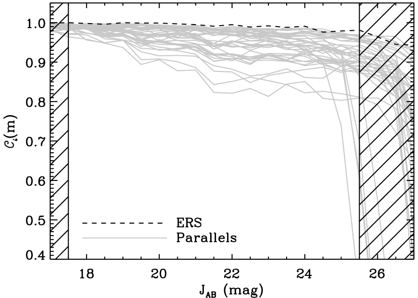
Figure 5.— The completeness corrections for the parallel (solid gray) and ERS field (dotted black). We estimate these corrections as the recovery rate of 1000 randomly-placed point sources in each magnitude interval. The completeness corrections are generally $\gtrsim\!90\%$ for our magnitude range and rarely tend to 100% (even at the bright-end), due to source blending.

We compute the model number counts for $240\!\leq\!z_{scl}\!\leq\!350$ pc with $\Delta z_{scl}\!=\!5$ pc and maximize the likelihood of obtaining the measured counts. Since the observed counts are in the limit of small integers, the probability distribution should be modeled as a Poisson distribution (Cash, 1979). To avoid confusion with the usual Gaussian probability distributions, we denote this goodness-of-fit statistic as $C^{2}$, and maximize the likelihood (${\cal L}$) in the usual way:

$$C^{2}(z_{scl}) = -2\ln\left(\prod_{m}{\cal L}\left(N_{m}\left|\hat{N}_{m}\right.\right)\right)$$ (13)

$$= -2\sum_{m}N_{m}\ln\left(\hat{N}_{m}\right)-\hat{N}_{m}-\ln\left(N_{m}!\right)$$ (14)

where $N_{m}$ and $\hat{N}_{m}$ are the observed and model differential number counts, respectively. Finally, we define $\Delta C^{2}\!\equiv\!C^{2}-\min(C^{2})$, which will follow the standard $\chi^{2}$-distribution (Cash, 1979) with one degree of freedom (in this case the scale height). In 6, we show the observed (solid histogram) and model counts (dashed line) for the optimal model of $z_{scl}\!=\!290$ with the total $1\sigma$ uncertainty (shaded region — we discuss our systematic uncertainties in § 5), as well as the $\Delta C^{2}(z_{scl})$ curve for $A_{J}\!=\!0$ mag in the inset (discussed in detail in § 5.1). We compute the random uncertainty on the scale height where $\Delta C^{2}\left(z_{scl}\right)\!=\!1$ to be $\pm 25$ pc.

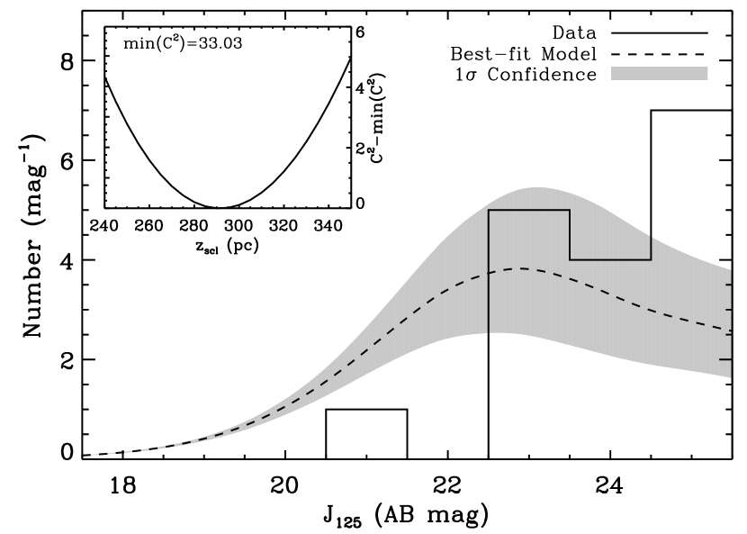
Figure 6.— Ultracool dwarf number counts. The histogram represents the number counts from 231.90 arcmin² from 39 parallel fields and the ERS data in the GOODS-S field. The solid line and grey region shows best-fitting model counts for $z_{scl}\!=\!290$ pc and the corresponding $1\sigma$ uncertainty, respectively. In the upper left, we show the $\Delta C^{2}(z_{scl})$ used to derive these scale height values. The peak in the model number counts at $J_{125}\!\sim\!24$ mag is not due to generic object incompleteness at the faint-end, but rather from having integrated completely through the disk.

5. Systematic Biases and Uncertainties

Here we discuss sources of potential systematic uncertainties that could affect our estimate of the vertical scale height.

5.1. Interstellar Extinction

As mentioned above, it is necessary to incorporate the field- and distance-dependent extinction to properly interpret the star counts. While the dust maps of Schlegel, Finkbeiner, & Davis (1998) provide the best estimate of the total line-of-sight Galactic extinction for extragalactic objects, they cannot be directly applied to our objects which reside within the Galaxy. Instead of parameterizing $A(\ell,b,R)$, we perform the above minimization for both $A(\ell,b,R)\!=\!0$ mag and the Schlegel, Finkbeiner, & Davis (1998) value as given in Table 1. As this approach brackets the two extinction extremes (the minimum and maximum extinction models, respectively), we expect it to indicate the degree to which insufficient knowledge of $A(\ell,b,R)$ is adversely affecting our results. Therefore we take the average and difference between the two extremal dust hypotheses as the expected value of the scale height, and its systematic uncertainty due to the extinction model, respectively. We approximate this as a symmetric uncertainty. However we do not expect these objects to be uniformly distributed between the two extinction limits. We find that the range of scale heights for the minimum and maximum extinction models is $\pm 5$ pc.

5.2. Ultracool Dwarf Luminosity Function

The measured ultracool dwarf luminosity function has potentially sizeable uncertainties ($\delta\Phi/\Phi\!\sim\!30$%), largely due to the Poisson counting uncertainty of these rare objects. To estimate the uncertainty introduced by the inaccurate knowledge of the luminosity function, we draw a normal random number for each absolute magnitude bin with mean and variance from the published results (e.g. Cruz et al., 2007; Reylé et al., 2010). We recompute the vertical scale height for 1000 realizations, and take the dispersion of optimal scale heights to be the systematic uncertainty. We estimate this uncertainty for our fields to be $\pm 30$ pc.

5.3. Malmquist Bias

For any flux-limited survey, intrinsically bright objects are preferentially detected, which biases the mean absolute magnitude ($\overline{M}$) as a function of apparent magnitude (Malmquist, 1936). Under basic assumptions, the correction to the absolute magnitudes is given by

$$\Delta M = \overline{M}-M_{0},$$ (15)

$$= -\frac{\sigma^{2}}{\log e}\frac{dN_{m}}{dm},$$ (16)

where $M_{0}$ is the intrinsic absolute magnitude, $\sigma$ is the dispersion on the brightnesses from the width of the main sequence and photometric uncertainties (e.g. Bochanski et al., 2010), and $\log e\!=\!0.4343$. Since our observed counts ($N_{m}$) are very discontinuous due to small number statistics, we opt to impose Malmquist bias on the model counts ($\hat{N}_{m}$). We adopt $\sigma\!=\!0.2$ mag which is a somewhat more conservative estimate than the typical photometric uncertainty of our faintest sources (see Table 3), which gives shifts on the absolute magnitude of $-0.1\!\lesssim\!\Delta M\!\lesssim\!0.2$ mag. Since this shift is considerably smaller than the width of our apparent magnitude bins, the bias on the vertical scale height is negligible.

5.4. Equal-Mass Binaries

We expect a fraction of our ultracool dwarfs will be in binary systems, which if unaccounted for, will tend to increase the vertical scale height measurements (e.g. Bochanski et al., 2010). To assess the properties of potential binary systems in our sample, we construct a grid of simulated images with two point sources placed at a range of separations ($1\!\leq\!s\!\leq\!5$ pix and $\Delta s\!=\!0.25$ pix), total magnitudes ($20\!\leq\!J_{125}\!\leq\!25$ mag and $\Delta J_{125}\!=\!0.25$ mag), and Gaussian noise field with mean and variance consistent with the parallel fields. For each brightness and separation, we generate 1000 realizations and catalog the images as described in § 2.3. We find that for separations of $s\!\lesssim\!3$ pix SExtractor does not detect two distinct point sources, but does recover the total flux to $\sim\!2$%. Furthermore, the combined source only fails to pass our axis ratio criterion of $(b/a)\!\leq\!0.7$ for $J_{125}\!\gtrsim\!23$ mag. Burgasser et al. (2007) find that most very low-mass stars have physical separations of $\Delta\!\lesssim\!20$ AU, which implies that the unresolved binaries that may escape our cataloging are at a distance of $50\!\lesssim\!R\!\lesssim\!80$ pc. Such systems will have an absolute magnitude of $M_{J}\!\gtrsim\!18$ AB mag, which corresponds to a spectral type that is far too cool to have been included in our sample (Hawley et al., 2002). Therefore we did not systematically reject any marginally-resolved binaries based on our axis ratio criterion.

Unresolved equal-mass binaries will be $2.5\log(2)$ mag brighter than a single star of the same spectral type and distance, which will skew the observed counts to brighter values and give the impression of a thinner disk (Bochanski et al., 2010). To estimate the magnitude of this effect, we randomly select a fraction of our objects (denoted as $f_{b}$) to be equal-mass binaries. We dim these objects by $2.5\log(2)$ mag, duplicate their entries in the number counts if the dimmed brightness is $J_{125}\!\leq\!25.5$ mag, and recompute the vertical scale height according to § 4. We repeat this procedure 1000 times for $f_{b}\!=\!0.1$, 0.2, 0.3, and 0.4 and find that the biases on the scale heights are $(z_{scl}^{\rm binary}-z_{scl})\!=\!5\pm 4$ pc, $6\pm 10$ pc, $14\pm 12$ pc, and $17\pm 12$ pc, respectively. The uncertainties in these biases reflect the distribution of estimated scale heights.

6. Discussion

With the deep ($J_{125}\!\lesssim\!26$ mag) HST/WFC3 parallel and pointed fields, we can identify an L0-dwarf out to $R\!\sim\!3.5$ kpc and a T0-dwarf to $\sim\!700$ pc. Since these fields are at high Galactic latitudes, they provide constraints on the vertical distribution of these intrinsically very faint objects. From our compilation of 231.90 arcmin² of HST imaging, we have identified 17 ultracool dwarf candidates, whose number counts are consistent with an exponential vertical distribution with a scale height of $z_{scl}\!=\!290\pm 25\;(\mathrm{random})\pm 31\;(\mathrm{systematic})$ pc. Our estimate improves upon previous results by combining the depths of Pirzkal et al. (2005) with the multiple sight-lines and area of Ryan et al. (2005). Additionally, our sample likely contains fewer M-dwarfs, owing to the deep infrared imaging. For example, the Ryan et al. (2005) work identified dwarfs later than $\sim\!\mathrm{M}6$ from HST/ACS parallels with a single color of $(i^{\prime}-z^{\prime})\!\geq\!1.3$ mag (see Bochanski et al., 2007, for representative SDSS colors of M-dwarfs). Since the early M-dwarfs are of considerably higher luminosity and far more common than the L-dwarfs, we speculate that the Ryan et al. (2005) sample contains many M-dwarfs. Using our derived Galactic structure model, we estimate that our sample contains $6.0\pm 2.2$, $7.4\pm 2.2$, and $2.3\pm 0.3$ M8–M9, L, and T-dwarfs, respectively. Had we adopted the weaker color criteria of Ryan et al. (2005), we would expect $27\pm 10$ M6–M9 dwarfs. Given these likely differences in sample properties, it is not surprising to find possible differences in the vertical scale height measurements. Finally, we note that the model counts peak around $J_{125}\!\simeq\!24$ mag, much brighter than the 50% completeness limit of $J_{125}\!\simeq\!26$ mag (see Table 1). This peak is not due to generic survey incompleteness at the faint-end, but rather due to the number density declining faster than the volume surveyed. At present, our observed number counts do not show or strongly demand such a peak, and more dwarfs at $J_{125}\!\sim\!24$ mag are needed to identify this critical peak.

We have used the most recent estimates of the ultracool dwarf luminosity function (e.g. Cruz et al., 2007; Reylé et al., 2010), which are derived primarily from nearby samples ($R\!\lesssim\!100$ pc). Since objects below the hydrogen-burning limit are passively-cooling, their bolometric luminosity strongly depends on their age and initial temperature. Therefore, the cooling will introduce a non-trivial time dependence on the luminosity function of a population of ultracool dwarfs (Burgasser, 2004c). For example, if the majority of these dwarfs are formed at the disk midplane and are scattered to these high Galactic latitudes by interactions with massive objects in the disk, then the luminosity function of these dwarfs is likely different than the local estimates, particularly if the cooling times are shorter than the scattering times. Specifically, many of the earliest L-dwarfs will have cooled to become later types, resulting in a more “bottom-heavy” luminosity function with respect to local estimates.

Additionally, this cooling should tend to make early- to mid-L dwarfs a kinematically younger population than the M-dwarfs Seifahrt et al. (e.g. 2010). However the high velocity dispersions reported by many kinematic studies suggest ages of 1–6 Gyr (e.g. Zapatero Osorio et al., 2007; Faherty et al., 2009; Seifahrt et al., 2010), with a well-established age of $\sim\!3$ Gyr for the M-dwarfs (e.g. Reid et al., 2002). If dwarfs immediately below the hydrogen-burning limit are indeed kinematically younger (and have a lower velocity dispersion) than the lowest mass main sequence dwarfs, then we expect they will be distributed in a thinner disk. Yet cooler spectral types will contain a mixture of old (high mass) dwarfs that have cooled and young (low mass) objects. This population will then be kinematically older, have a higher velocity dispersion, and reside in a thicker disk than the warmest brown dwarfs. Therefore we expect to see a gradual deviation in the trend of scale height with spectral type, since the hydrogen-burning limit does not occur for a fixed spectral type. With the present data, we find a scale height of $z_{scl}\!=\!290\pm 40$ pc for a sample of M8–T dwarfs, which is comparable to estimates for mid-M dwarfs (Jurić et al., 2008; Bochanski et al., 2010) and is qualitatively consistent with the kinematic results (e.g. Faherty et al., 2009). However, our estimate is somewhat lower than the extrapolation of the trend of scale height with spectral type (see Figure 10 of Jurić et al., 2008). More data with greatly improved spectral typing is needed to fully constrain these effects.

Our sample may contain dwarfs as early as $\sim$M8, which is a direct consequence of the filter set. These infrared colors are determined mostly by a series of molecular absorption bands, notably H₂O and CH₄, which are in turn used to define the spectral types (e.g. Kirkpatrick, 2005, and references therein). Therefore, a cleaner selection and spectral typing can be achieved by using medium or narrow bands which isolate these spectral features (e.g. Jones et al., 1994). For example, the H₂O feature at $\lambda\!=\!1.34~{}\mu$m directly maps onto effective temperature (Jones et al., 1995) and is relatively insensitive to surface gravity and metallicity (Gorlova et al., 2003; Wilking et al., 2004). Unfortunately the $J_{125}$- and $H_{160}$-bands equally split the H₂O feature, diminishing the type discrimination of the $(J_{125}-H_{160})$ color. Future surveys dedicated to finding ultracool dwarfs could take advantage of these molecular features for robust identification and classification. Fortunately, WFC3 contains a host of filters designed to sample this H₂O absorption feature (Lupie & Boucarut, 2000), specifically F127M, F139M, and F153M. Furthermore, the James Webb Space Telescope (JWST) and its Near-Infrared Camera (NIRCam) will be equipped with similar bandpasses, but with a significantly larger collecting area facilitating surveys at still larger heliocentric distances and search for ultracool dwarfs associated with other Galactic components (such as thick disk, halo, or bulge).

References

- Bahcall (1986) Bahcall, J. N. 1986, ARA&A, 24, 577
- Bahcall & Soneira (1980) Bahcall, J. N. & Soniera, R. M. 1980, ApJS, 44, 73
- Bahcall & Soneira (1984) Bahcall, J. N. & Soniera, R. M. 1984, ApJS, 55, 67
- Beckwith et al. (2006) Beckwith, S. V. W., et al. 2006, AJ, 132, 1729
- Bertin & Arnouts (1996) Berin, E. & Arnouts, S. 1996, A&AS, 117, 393
- Bochanski et al. (2007) Bochanski, J. J., West, A. A., Hawley, S. L., & Covey, K. R. 2007, AJ, 133, 531
- Bochanski et al. (2010) Bochanski, J. J., Hawley, S. L., Covey, K. R., West, A. A., Reid, I. N., Golimowski, D. A., & Ivezić, Ž. 2010, AJ, 139, 2679
- Bok (1937) Bok, B. J. 1937, The Distribution of Stars in Space. Chicago: University of Chicago Press
- Bouwens et al. (2006) Bouwens, R. J., Illingworth, G. D., Blakeslee, J. P., & Franx, M. 2006, ApJ, 653, 53
- Bouwens et al. (2010) Bouwens, R. J., et al. 2010, arXiv: 1006.4360
- Burgasser et al. (2004a) Burgasser, A. J., McElwain, M. W., Kirkpatrick, J. D., Cruz, K. L., Tinney, C. G., Reid, I. N. 2004a, AJ, 127, 2856
- Burgasser et al. (2004b) Burgasser, A. J. 2004b, ApJ, 614, L73
- Burgasser (2004c) Burgasser, A. J. 2004c, ApJS, 155, 191
- Burgasser et al. (2006a) Burgasser, A. J., Geballe, T. R., Leggett, S. K., Kirkpatrick, J. D., & Golimowski, D. A. 2006a, ApJ, 637, 1067