Characters of symmetric groups in terms of free cumulants and Frobenius coordinates

Abstract

Free cumulants are nice and useful functionals of the shape of a Young diagram, in particular they give the asymptotics of normalized characters of symmetric groups $\mathfrak{S}(n)$ in the limit $n\to\infty$. We give an explicit combinatorial formula for normalized characters of the symmetric groups in terms of free cumulants. We also express characters in terms of Frobenius coordinates. Our formulas involve counting certain factorizations of a given permutation. The main tool are Stanley polynomials which give values of characters on multirectangular Young diagrams.

Résumé. Les cumulants libres sont des fonctions agréables et utiles sur l’ensemble des diagrammes de Young, en particulier, ils donnent le comportement asymptotiques des caractères normalisés du groupe symétrique $\mathfrak{S}(n)$ dans la limite $n\to\infty$. Nous donnons une formule combinatoire explicite pour les caractères normalisés du groupe symétrique en fonction des cumulants libres. Nous exprimons également les caractères en fonction des coordonnées de Frobenius. Nos formules font intervenir le nombre de certaines factorisations d’une permutation donnée. L’outil principal est la famille de polynômes de Stanley donnant les valeurs des caractères sur les diagrammes de Young multirectangulaires.

Figure 1: Young diagram $(4,3,1)$ drawn in the French convention

1 Introduction

This contribution is an extended abstract of a full version [DFŚ10] which will be published elsewhere.

1.1 Dilations of Young diagrams and normalized characters

For a Young diagram $\lambda$ and an integer $s\geq 1$ we denote by $s\lambda$ the dilation of $\lambda$ by factor $s$. This operation can be easily described on a graphical representation of a Young diagram: we just dilate the picture of $\lambda$ or, alternatively, we replace each box of $\lambda$ by a grid of $s\times s$ boxes.

Any permutation $\pi\in\mathfrak{S}(k)$ can be also regarded as an element of $\mathfrak{S}(n)$ if $k\leq n$ (we just declare that $\pi\in\mathfrak{S}(n)$ has additional $n-k$ fixpoints). For any $\pi\in\mathfrak{S}(k)$ and an irreducible representation $\rho^{\lambda}$ of the symmetric group $\mathfrak{S}(n)$ corresponding to the Young diagram $\lambda$ we define the normalized character

$$\Sigma^{\lambda}_{\pi}=\begin{cases}\underbrace{n(n-1)\cdots(n-k+1)}_{k\text{ factors}}\frac{\operatorname{Tr}\rho^{\lambda}(\pi)}{\text{dimension of $\rho^{\lambda}$}}&\text{if }k\leq n,\\ 0&\text{otherwise.}\end{cases}$$

We shall concentrate our attention on the characters on cycles, therefore we will use the special notation

$$\Sigma^{\lambda}_{k}=\Sigma^{\lambda}_{(1,2,\dots,k)},$$

where we treat the cycle $(1,2,\dots,k)$ as an element of $\mathfrak{S}(k)$ for any integer $k\geq 1$.

The notion of dilation of a Young diagram is very useful from the viewpoint of the asymptotic representation theory because it allows us to ask the following question:

Problem 1

What can we say about the characters of the symmetric groups in the limit when the Young diagram $\lambda$ tends in some sense to infinity in a way that $\lambda$ preserves its shape?

This informal problem can be formalized as follows: for fixed $\lambda$ and $k$ we ask about (asymptotic) properties of the normalized characters $\Sigma^{s\lambda}_{k}$ in the limit $s\to\infty$. The reason why we decided to study this particular normalization of characters is the following well-known yet surprising result.

Fact 2

For any Young diagram $\lambda$ and integer $k\geq 2$ the normalized character on a dilated diagram

$$\mathbb{N}\ni s\mapsto\Sigma^{s\lambda}_{k-1}$$ (1)

is a polynomial function of degree (at most) $k$.

1.2 Generalized Young diagrams

Any Young diagram drawn in the French convention can be identified with its graph which is equal to the set $\{(x,y):0\leq x,0\leq y\leq f(x)\}$ for a suitably chosen function $f:\mathbb{R}_{+}\rightarrow\mathbb{R}_{+}$, where $\mathbb{R}_{+}=[0,\infty)$, cf. Figure 1. It is therefore natural to define the set of generalized Young diagrams $\mathbb{Y}$ (in the French convention) as the set of bounded, non-increasing functions $f:\mathbb{R}_{+}\rightarrow\mathbb{R}_{+}$ with a compact support; in this way any Young diagram can be regarded as a generalized Young diagram. Notice that with the notion of generalized Young diagrams we may consider dilations $s\lambda$ for any real $s\geq 0$.

1.3 How to describe the shape of a Young diagram?

Our ultimate goal is to explicitly express the polynomials (1) in terms of the shape of $\lambda$. However, before we start this task we must ask ourselves: how to describe the shape of $\lambda$ in the best way? In the folowing we shall present two approaches to this problem.

We define the fundamental functionals of shape of a Young diagram $\lambda$ by an integral over the area of $\lambda$

$$S^{\lambda}_{k}=(k-1)\iint_{(x,y)\in\lambda}(\operatorname{contents}_{(x,y)})^{k-2}\ dx\ dy$$

for integer $k\geq 2$, and where $\operatorname{contents}_{(x,y)}=x-y$ is the contents of a point of a Young diagram. When it does not lead to confusions we will skip the explicit dependence of the fundamental functionals on Young diagrams and instead of $S^{\lambda}_{k}$ we shall simply write $S_{k}$. Clearly, each functional $S_{k}$ is a homogeneous function of the Young diagram with degree $k$, i.e. $S^{s\lambda}_{k}=s^{k}S^{\lambda}_{k}$.

For a Young diagram with Frobenius coordinates $\lambda=\begin{bmatrix}a_{1}&\cdots&a_{l}\\ b_{1}&\cdots&b_{l}\end{bmatrix}$ we define its shifted Frobenius coordinates with $A_{i}=a_{i}+\frac{1}{2}$ and $B_{i}=b_{i}+\frac{1}{2}$. Shifted Frobenius coordinates have a simple interpretation as positions (up to the sign) of the particles and holes in the Dirac sea corresponding to a Young diagram [Oko01]. Functionals $S^{\lambda}_{k}$ can be nicely expressed in terms of (shifted) Frobenius coordinates as follows:

$$S^{\lambda}_{k}=\sum_{i}\int_{-\frac{1}{2}}^{\frac{1}{2}}\left[(A_{i}+z)^{k-1}-(-B_{i}-z)^{k-1}\right]dz,$$

$$\frac{S^{\lambda}_{k}}{|\lambda|^{k-1}}=\sum_{i}\left[\alpha_{i}^{k-1}-(-\beta_{i})^{k-1}\right]+O\left(\frac{1}{|\lambda|^{2}}\right),\qquad\text{where $\alpha_{i}=\frac{A_{i}}{|\lambda|}$ and $\beta_{i}=\frac{B_{i}}{|\lambda|}$.}$$ (2)

Another way of describing the shape of a Young diagram $\lambda$ is to use its free cumulants $R_{2}^{\lambda},R_{3}^{\lambda},\dots$ which are defined as the coefficients of the leading terms of the polynomials (1):

$$R_{k}^{\lambda}=[s^{k}]\Sigma^{s\lambda}_{k-1}=\lim_{s\to\infty}\frac{1}{s^{k}}\Sigma^{s\lambda}_{k-1}\qquad\text{for integer $k\geq 2$}.$$

Later on we shall show how to calculate free cumulants directly from the shape of a Young diagram. $R_{k}$ is a homogeneous function of the Young diagram with degree $k$, i.e. $R^{s\lambda}_{k}=s^{k}R^{\lambda}_{k}$.

The importance of homogeneity of $S_{k}^{\lambda}$ and $R_{k}^{\lambda}$ becomes clear when one wants to solve asymptotic problems, such as understanding coefficients of the polynomial (1).

1.4 Character polynomials and their applications

It is not very difficult to show [DFŚ10] that for each integer $k\geq 1$ there exists a polynomial with rational coefficients $J_{k}(S_{2},S_{3},\dots)$ with a property that

$$\Sigma_{k}^{\lambda}=J_{k}(S_{2}^{\lambda},S_{3}^{\lambda},\dots)$$

holds true for any Young diagram $\lambda$. For example, we have

$$\Sigma_{1}=S_{2},\qquad\Sigma_{2}=S_{3},\qquad\Sigma_{3}=S_{4}-\frac{3}{2}S_{2}^{2}+S_{2},\qquad\Sigma_{4}=S_{5}-4S_{2}S_{3}+5S_{3},$$

$$\Sigma_{5}=S_{6}-5S_{2}S_{4}-\frac{5}{2}S_{3}^{2}+\frac{25}{6}S_{2}^{3}+15S_{4}-\frac{35}{2}S_{2}^{2}+8S_{2}.$$

The polynomials $J_{n}$ are very useful, when one studies the asymptotics of characters in the limit when the parameters $\alpha_{1},\alpha_{2},\dots,\beta_{1},\beta_{2},\dots$ converge to some limits and the number of boxes of $\lambda$ tends to infinity. Equation (2) shows that for such scaling it is convenient to consider a different gradation, in which the degree of $S_{k}$ is equal to $k-1$. We leave it as an exercise to the Reader to use the results of this paper to show that with respect to this gradation polynomial $J_{k}$ has the form

$$\Sigma_{k}=S_{k+1}-\frac{k}{2}\sum_{j_{1}+j_{2}=k+1}S_{j_{1}}S_{j_{2}}+\text{(terms of smaller degree)}.$$

The dominant part of the right-hand side (the first summand) coincides with the estimate of Wassermann [Was81] and with Thoma character on $\mathfrak{S}(\infty)$ [VK81]. In a similar way it is possible to obtain next terms in the expansion.

One can also show that for each integer $k\geq 1$ there exists a polynomial with integer coefficients $K_{k}(R_{2},R_{3},\dots)$, called Kerov character polynomial [Ker00, Bia03] with a property that

$$\Sigma_{k}^{\lambda}=K_{k}(R_{2}^{\lambda},R_{3}^{\lambda},\dots)$$

holds true for any Young diagram $\lambda$. For example,

$$\Sigma_{1}=R_{2},\qquad\Sigma_{2}=R_{3},\qquad\Sigma_{3}=R_{4}+R_{2},\qquad\Sigma_{4}=R_{5}+5R_{3},$$

$$\Sigma_{5}=R_{6}+15R_{4}+5R_{2}^{2}+8R_{2},\qquad\Sigma_{6}=R_{7}+35R_{5}+35R_{3}R_{2}+84R_{3}.$$

The advantage of Kerov polynomials $K_{k}$ over polynomials $J_{k}$ comes from the fact that they usually have a much simpler form, involve smaller number of summands and are more suitable for studying asymptotics of characters in the case of balanced Young diagrams, i.e. for example in the case of characters $\Sigma^{s\lambda}_{k}$ of dilated Young diagrams [Bia03].

1.5 The main result: explicit form of character polynomials

For a permutation $\pi$ we denote by $C(\pi)$ the set of the cycles of $\pi$.

Theorem 3 (Dołęga, Féray, Śniady [DFŚ10])

The coefficients of polynomials $J_{k}$ are explicitly described as follows:

$$\left.\frac{\partial}{\partial S_{j_{1}}}\cdots\frac{\partial}{\partial S_{j_{l}}}J_{k}\right|_{S_{2}=S_{3}=\cdots=0}$$

is equal to $(-1)^{l-1}$ times the number of the number of the triples $(\sigma_{1},\sigma_{2},\ell)$ where

• $\sigma_{1},\sigma_{2}\in\mathfrak{S}(k)$ are such that $\sigma_{1}\circ\sigma_{2}=(1,2,\dots,k)$,

• $\ell:C(\sigma_{2})\rightarrow\{1,\dots,l\}$ is a bijective labeling,

• for each $1\leq i\leq l$ there are exactly $j_{i}-1$ cycles of $\sigma_{1}$ which intersect cycle $\ell^{-1}(i)$ and which do not intersect any of the cycles $\ell^{-1}(i+1),\ell^{-1}(i+2),\dots$.

Theorem 4 (Dołęga, Féray, Śniady [DFŚ10])

The coefficient of $R_{2}^{s_{2}}R_{3}^{s_{3}}\cdots$ in the Kerov polynomial $K_{k}$ is equal to the number of triples $(\sigma_{1},\sigma_{2},q)$ with the following properties:

1. $\sigma_{1},\sigma_{2}\in\mathfrak{S}(k)$ are such that $\sigma_{1}\circ\sigma_{2}=(1,2,\dots,k)$;

2. the number of cycles of $\sigma_{2}$ is equal to the number of factors in the product $R_{2}^{s_{2}}R_{3}^{s_{3}}\cdots$; in other words $|C(\sigma_{2})|=s_{2}+s_{3}+\cdots$;

3. the total number of cycles of $\sigma_{1}$ and $\sigma_{2}$ is equal to the degree of the product $R_{2}^{s_{2}}R_{3}^{s_{3}}\cdots$; in other words $|C(\sigma_{1})|+|C(\sigma_{2})|=2s_{2}+3s_{3}+4s_{4}+\cdots$;

4. $q:C(\sigma_{2})\rightarrow\{2,3,\dots\}$ is a coloring of the cycles of $\sigma_{2}$ with a property that each color $i\in\{2,3,\dots\}$ is used exactly $s_{i}$ times (informally, we can think that $q$ is a map which to cycles of $C(\sigma_{2})$ associates the factors in the product $R_{2}^{s_{2}}R_{3}^{s_{3}}\cdots$);

5. for every set $A\subset C(\sigma_{2})$ which is nontrivial (i.e., $A\neq\emptyset$ and $A\neq C(\sigma_{2})$) there are more than $\sum_{i\in A}\big{(}q(i)-1\big{)}$ cycles of $\sigma_{1}$ which intersect $\bigcup A$.

Only condition (e) is rather complicated, therefore we will provide two equivalent combinatorial conditions below.

1.6 Marriage and transportation interpretations of condition (e)

Let $(\sigma_{1},\sigma_{2},q)$ be a triple which fulfills conditions (a)–(d) of Theorem 4. We consider the following polyandrous interpretation of Hall marriage theorem. Each cycle of $\sigma_{1}$ will be called a boy and each cycle of $\sigma_{2}$ will be called a girl. For each girl $j\in C(\sigma_{2})$ let $q(j)-1$ be the desired number of husbands of $j$. We say that a boy $i\in C(\sigma_{1})$ is a possible candidate for a husband for a girl $j\in C(\sigma_{2})$ if cycles $i$ and $j$ intersect. Hall marriage theorem applied to our setup says that there exists an arrangement of marriages $\mathcal{M}:C(\sigma_{1})\rightarrow C(\sigma_{2})$ which assigns to each boy his wife (so that each girl $j$ has exactly $q(j)-1$ husbands) if and only if for every set $A\subseteq C(\sigma_{2})$ there are at least $\sum_{i\in A}\big{(}q(i)-1\big{)}$ cycles of $\sigma_{1}$ which intersect $\bigcup A$. As one easily see, the above condition is similar but not identical to (e). The following Proposition shows the connection between these two problems.

Proposition 5

Condition (e) is equivalent to each of the following two conditions:

1. for every nontrivial set of girls $A\subset C(\sigma_{2})$ (i.e., $A\neq\emptyset$ and $A\neq C(\sigma_{2})$) there exist two ways of arranging marriages $\mathcal{M}_{p}:C(\sigma_{1})\rightarrow C(\sigma_{2})$, $p\in\{1,2\}$ for which the corresponding sets of husbands of wives from $A$ are different:

   $$\mathcal{M}_{1}^{-1}(A)\neq\mathcal{M}_{2}^{-1}(A),$$

1. there exists a strictly positive solution to the following system of equations:

   Set of variables

   $\big{\{}x_{i,j}:\text{ $i\in C(\sigma_{1})$ and $j\in C(\sigma_{2})$ are intersecting cycles}\big{\}}$

   Equations

   $\left\{\begin{array}[]{l}\forall i,\sum_{j}x_{i,j}=1\\ \forall j,\sum_{i}x_{i,j}=q(j)-1\end{array}\right.$

Note that the possibility of arranging marriages can be rephrased as existence of a solution to the above system of equations with a requirement that $x_{i,j}\in\{0,1\}$.

The system of equations in condition (e³) can be interpreted as a transportation problem where each cycle of $\sigma_{1}$ is interpreted as a factory which produces a unit of some ware and each cycle $j$ of $\sigma_{2}$ is interpreted as a consumer with a demand equal to $q(j)-1$. The value of $x_{i,j}$ is interpreted as amount of ware transported from factory $i$ to the consumer $j$.

1.7 General conjugacy classes

An analogue of Theorem 3 holds true with some minor modifications also for the analogues of polynomials $J$ giving the values of characters on general permutations, not just cycles.

In case of the analogues of the Kerov polynomials giving the values of characters on more complex permutations $\pi$ than cycles the situation is slightly more diffcult. Namely, an analogue of Theorem 4 holds true if the character $\Sigma_{\pi}$ is replaced by some quantities which behave like classical cumulants of cycles constituting $\pi$ and the sum on the right-hand side is taken only over transitive factorizations. Since the expression of characters in terms of classical cumulants of cycles is straightforward, we obtain an expression of characters in terms of free cumulants.

1.8 Applications of the main result

The results of this article (Theorem 4 in particular) can be used to obtain new asymptotic inequalities for characters of the symmetric groups. This vast topic is outside of the scope of this article and will be studied in a subsequent paper.

1.9 Contents of this article

In this article we shall prove Theorem 3. Also, since the proof of Theorem 4 is rather long and technical [DFŚ10], in this overview article we shall highlight just the main ideas and concentrate on the first non-trivial case of quadratic terms of Kerov polynomials.

Due to lack of space we were not able to show the full history of the presented results and to give to everybody the proper credits. For more history and bibliographical references we refer to the full version of this article [DFŚ10].

2 Ingredients of the proof of the main result

2.1 Polynomial functions on the set of Young diagrams

Surprisingly, the normalized characters $\Sigma_{\pi}^{\lambda}$ can be extended in a natural way for any generalized Young diagram $\lambda\in\mathbb{Y}$. The algebra they generate will be called algebra of polynomial functions on (generalized) Young diagrams. It is well-known that many natural families of functions on Young diagrams generate the same algebra, for example the family of free cumulants $(R_{k}^{\lambda})$ or the family of fundamental functionals $(S_{k}^{\lambda})$.

2.2 Stanley polynomials

For two finite sequences of positive real numbers $\mathbf{p}=(p_{1},\dots,p_{m})$ and $\mathbf{q}=(q_{1},\dots,q_{m})$ with $q_{1}\geq\cdots\geq q_{m}$ we consider a multirectangular generalized Young diagram $\mathbf{p}\times\mathbf{q}$, cf Figure 2. In the case when $p_{1},\dots,p_{m},q_{1},\dots,q_{m}$ are natural numbers $\mathbf{p}\times\mathbf{q}$ is a partition

$$\mathbf{p}\times\mathbf{q}=(\underbrace{q_{1},\dots,q_{1}}_{p_{1}\text{ times}},\underbrace{q_{2},\dots,q_{2}}_{p_{2}\text{ times}},\dots).$$

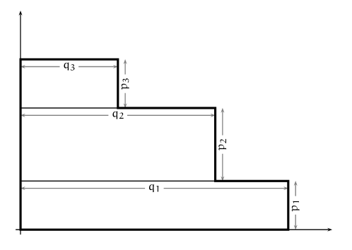
Figure 2: Generalized Young diagram $\mathbf{p}\times\mathbf{q}$ drawn in the French convention

Proposition 6

Let $\mathcal{F}:\mathbb{Y}\rightarrow\mathbb{R}$ be a polynomial function on the set of generalized Young diagrams. Then $(\mathbf{p},\mathbf{q})\mapsto\mathcal{F}(\mathbf{p}\times\mathbf{q})$ is a polynomial in indeterminates $p_{1},\dots,p_{m},q_{1},\dots,q_{m}$, called Stanley polynomial.

Proof 2.1.

It is enough to prove this proposition for some family of generators of the algebra of polynomial functions on $\mathbb{Y}$. In the case of functionals $S_{2},S_{3},\dots$ it is a simple exercise.

Lemma 2.2.

If we treat $\mathbf{p}$ as variables and $\mathbf{q}$ as constants then for every $k\geq 2$ and all $i_{1}<\cdots<i_{s}$

$$[p_{i_{1}}\cdots p_{i_{s}}]S_{k}^{\mathbf{p}\times\mathbf{q}}=\begin{cases}(-1)^{s-1}\ (k-1)_{s-1}\ q_{i_{s}}^{k-s}&\text{if\/ $1\leq s\leq k-1$},\\ 0&\text{otherwise}.\end{cases}$$ (3)

Proof 2.3.

The integral over the Young diagram $\mathbf{p}\times\mathbf{q}$ can be split into several integrals over rectangles constituting $\mathbf{p}\times\mathbf{q}$ therefore

$$S_{k}^{\mathbf{p}\times\mathbf{q}}=(k-1)\iint_{(x,y)\in\mathbf{p}\times\mathbf{q}}(x-y)^{k-2}\ dx\ dy=\\ (k-1)!\sum_{1\leq r\leq k-1}(-1)^{r-1}\iint_{(x,y)\in\mathbf{p}\times\mathbf{q}}\frac{x^{k-1-r}}{(k-1-r)!}\frac{y^{r-1}}{(r-1)!}\ dx\ dy=\\ (k-1)!\sum_{1\leq r\leq k-1}(-1)^{r-1}\sum_{j}\frac{q_{j}^{k-r}}{(k-r)!}\frac{(p_{1}+\cdots+p_{j})^{r}-(p_{1}+\cdots+p_{j-1})^{r}}{r!}.$$

For any $i_{1}<\cdots<i_{s}$

$$\left.\frac{\partial^{s}}{\partial p_{i_{1}}\cdots\partial p_{i_{s}}}\frac{(p_{1}+\cdots+p_{j})^{r}-(p_{1}+\cdots+p_{j-1})^{r}}{r!}\right|_{p_{1}=p_{2}=\cdots=0}=\begin{cases}1&\text{if $s=r$ and $i_{s}=j$,}\\ 0&\text{otherwise}\end{cases}$$

which finishes the proof.

Theorem 2.3.

Let $\mathcal{F}:\mathbb{Y}\rightarrow\mathbb{R}$ be a polynomial function on the set of generalized Young diagrams, we shall view it as a polynomial in $S_{2},S_{3},\dots$ Then for any $j_{1},\dots,j_{l}\geq 2$

$$\left.\frac{\partial}{\partial S_{j_{1}}}\cdots\frac{\partial}{\partial S_{j_{l}}}\mathcal{F}\right|_{S_{2}=S_{3}=\cdots=0}=[p_{1}q_{1}^{j_{1}-1}\cdots p_{l}q_{l}^{j_{l}-1}]\mathcal{F}^{\mathbf{p}\times\mathbf{q}}.$$

Proof 2.4.

By linearity is enough to consider the case when $\mathcal{F}=S_{m_{1}}\cdots S_{m_{r}}$. Clearly, the left hand side is equal to the number of permutations of the sequence $(m_{1},\dots,m_{r})$ which are equal to the sequence $(j_{1},\dots,j_{l})$. Lemma 2.2 shows that the same holds true for the right-hand side.

Corollary 2.5.

If $j_{1},\dots,j_{l}\geq 2$ then

$$[p_{1}q_{1}^{j_{1}-1}\cdots p_{l}q_{l}^{j_{l}-1}]\mathcal{F}^{\mathbf{p}\times\mathbf{q}}$$

does not depend on the order of the elements of the sequence $(j_{1},\dots,j_{l})$.

2.3 Stanley polynomials for characters

The following theorem gives explicitly the Stanley polynomial for normalized characters of symmetric groups. It was conjectured by Stanley [Sta06] and proved by Féray [Fér10] and therefore we refer to it as Stanley-Féray character formula. For a more elementary proof we refer to [FŚ11].

Theorem 2.5.

The value of the normalized character on $\pi\in\mathfrak{S}(k)$ for a multirectangular Young diagram $\mathbf{p}\times\mathbf{q}$ for $\mathbf{p}=(p_{1},\dots,p_{r})$, $\mathbf{q}=(q_{1},\dots,q_{r})$ is given by

$$\Sigma^{\mathbf{p}\times\mathbf{q}}_{\pi}=\sum_{\begin{subarray}{c}\sigma_{1},\sigma_{2}\in\mathfrak{S}(k)\\ \sigma_{1}\circ\sigma_{2}=\pi\end{subarray}}\ \sum_{\phi_{2}:C(\sigma_{2})\rightarrow\{1,\dots,r\}}(-1)^{\sigma_{1}}\left[\prod_{b\in C(\sigma_{1})}q_{\phi_{1}(b)}\prod_{c\in C(\sigma_{2})}p_{\phi_{2}(c)}\right],$$ (4)

where $\phi_{1}:C(\sigma_{1})\rightarrow\{1,\dots,r\}$ is defined by

$$\phi_{1}(c)=\max_{\begin{subarray}{c}b\in C(\sigma_{2}),\\ \text{$b$ and $c$ intersect}\end{subarray}}\phi_{2}(b).$$

Notice that Theorem 2.3 and the above Theorem 2.5 give immediately the proof of Theorem 3.

2.4 Relation between free cumulants and fundamental functionals

Corollary 2.6.

The value of the $k$-th free cumulant for a multirectangular Young diagram $\mathbf{p}\times\mathbf{q}$ for $\mathbf{p}=(p_{1},\dots,p_{r})$, $\mathbf{q}=(q_{1},\dots,q_{r})$ is given by

$$R^{\mathbf{p}\times\mathbf{q}}_{k}=\sum_{\begin{subarray}{c}\sigma_{1},\sigma_{2}\in\mathfrak{S}(k-1)\\ \sigma_{1}\circ\sigma_{2}=(1,2,\dots,k-1)\\ |C(\sigma_{1})|+|C(\sigma_{2})|=k\end{subarray}}\ \sum_{\phi_{2}:C(\sigma_{2})\rightarrow\{1,\dots,r\}}(-1)^{\sigma_{1}}\left[\prod_{b\in C(\sigma_{1})}q_{\phi_{1}(b)}\prod_{c\in C(\sigma_{2})}p_{\phi_{2}(c)}\right],$$ (5)

where $\phi_{1}:C(\sigma_{1})\rightarrow\{1,\dots,r\}$ is defined as in Theorem 2.5.

Proof 2.7.

It is enough to consider the homogeneous part with degree $k$ of both sides of (4) for $\pi=(1,\dots,k-1)\in\mathfrak{S}(k-1)$.

Proposition 2.8.

For any integer $n\geq 2$

$$R_{k}=\sum_{l\geq 1}\frac{1}{l!}(-k+1)^{l-1}\sum_{\begin{subarray}{c}j_{1},\dots,j_{l}\geq 2\\ j_{1}+\cdots+j_{l}=k\end{subarray}}S_{j_{1}}\cdots S_{j_{l}}.$$

Before the proof notice that the above formula shows that free cumulants can be explicitly and directly calculated from the shape of a Young diagram.

Proof 2.9.

For simplicity, we shall proof a weaker form of this result, namely

$$R_{k}=S_{k}-\frac{k-1}{2}\sum_{j_{1}+j_{2}=k}S_{j_{1}}S_{j_{2}}+\text{(terms involving at least three factors $S_{j}$)}.$$ (6)

Theorem 2.3 shows that the expansion of $R_{k}$ in terms of $(S_{j})$ involves coefficients of Stanley polynomials and the latter are given by Corollary 2.6. We shall use this idea in the following.

Notice that the condition $|C(\sigma_{1})|+|C(\sigma_{2})|=k$ appearing in (5) is equivalent to $|\sigma_{1}|+|\sigma_{2}|=|\sigma_{1}\circ\sigma_{2}|$ where $|\pi|$ denotes the length of the permutation, i.e. the minimal number of factors necessary to write $\pi$ as a product of transpositions. In other words, $\pi_{1}\circ\pi_{2}=(1,\dots,k-1)$ is a minimal factorization of a cycle. Such factorizations are in a bijective correspondence with non-crossing partitions of $k-1$-element set [Bia96]. It is therefore enough to enumerate appropriate non-crossing partitions. We present the details of this reasoning below.

The linear term $[S_{k}]R_{k}=[p_{1}q_{1}^{k-1}]R^{\mathbf{p}\times\mathbf{q}}_{k}$ is equal to the number of minimal factorizations such that $\sigma_{2}$ consists of one cycle and $\sigma_{1}$ consists of $k-1$ cycles. Such factorizations corresponds to non-crossing partitions of $k-1$ element set which have exactly one block and clearly there is only one such partition.

Since both free cumulants $(R_{j})$ and fundamental functionals of shape are homogeneous, by comparing the degrees we see that $[S_{j}]R_{k}=0$ if $j\neq k$. The same argument shows that $[S_{j_{1}}S_{j_{2}}]R_{k}=0$ if $j_{1}+j_{2}\neq k$.

Instead of finding the quadratic terms $[S_{j_{1}}S_{j_{2}}]R_{k}$ is better to find the derivative $\left.\frac{\partial^{2}}{\partial S_{j_{1}}\partial S_{j_{2}}}R_{k}\right|_{S_{j_{1}}=S_{j_{2}}=0}$ since it better takes care of the symmetric case $j_{1}=j_{2}$. The latter derivative is equal (up to the sign) to the number of minimal factorizations such that $\sigma_{2}$ consists of two labeled cycles $c_{1},c_{2}$ and $\sigma_{1}$ consists of $k-2$ cycles. Furthermore, we require that there are $j_{2}-1$ cycles of $\sigma_{1}$ which intersect cycle $c_{2}$. This is equivalent to counting non-crossing partitions of $k-1$-element set which consist of two labeled blocks $b_{1},b_{2}$ and we require that the block $b_{2}$ consists of $j_{2}-1$ elements. It is easy to see that all such non-crossing partitions can be transformed into each other by a cyclic rotation hence there are $k-1$ of them which finishes the proof.

The general case can be proved by analogous but more technically involved combinatorial considerations.

2.5 Identities fulfilled by coefficients of Stanley polynomials

The coefficients of Stanley polynomials $[p_{1}^{s_{1}}q_{1}^{r_{1}}\cdots]\mathcal{F}^{\mathbf{p}\times\mathbf{q}}$ for a polynomial function $\mathcal{F}$ are not linearly independent; in fact they fulfill many identities. In the following we shall show just one of them.

Lemma 2.10.

For any polynomial function $\mathcal{F}:\mathbb{Y}\rightarrow\mathbb{R}$

$$(j_{1}+j_{2}-1)\left[p_{1}q_{1}^{j_{1}+j_{2}-1}\right]\mathcal{F}^{\mathbf{p}\times\mathbf{q}}=-\left[p_{1}p_{2}q_{2}^{j_{1}+j_{2}-2}\right]\mathcal{F}^{\mathbf{p}\times\mathbf{q}}.$$ (7)

Proof 2.11.

It is enough to prove the Lemma if $\mathcal{F}=S_{k_{1}}\dots S_{k_{r}}$ is a monomial in fundamental functionals. Lemma 2.2 shows that the left-hand side of (7) is non-zero only if $\mathcal{F}=S_{j_{1}+j_{2}}$ (it is also a consequence of Theorem 2.3); otherwise every monomial in $\mathbf{p}$ and $\mathbf{q}$ with a nonzero coefficient would be at least quadratic with respect to the variables $\mathbf{p}$. The same argument shows that if the right-hand side is non-zero then either $\mathcal{F}=S_{k}$ is linear (in this case $k=j_{1}+j_{2}$ by comparing the degrees) or $\mathcal{F}=S_{k_{1}}S_{k_{2}}$ is quadratic. In the latter case, an inspection of the coefficient

$$[p_{1}p_{2}]S^{\mathbf{p}\times\mathbf{q}}_{k_{1}}S_{k_{2}}^{\mathbf{p}\times\mathbf{q}}=[p_{1}]S^{\mathbf{p}\times\mathbf{q}}_{k_{1}}\cdot[p_{2}]S^{\mathbf{p}\times\mathbf{q}}_{k_{2}}+[p_{1}]S^{\mathbf{p}\times\mathbf{q}}_{k_{2}}\cdot[p_{2}]S^{\mathbf{p}\times\mathbf{q}}_{k_{1}}=q_{1}^{k_{1}-1}q_{2}^{k_{2}-1}+q_{1}^{k_{2}-1}q_{2}^{k_{1}-1}$$

thanks to (3) leads to a contradiction.

It remains to show that for $\mathcal{F}=S_{j_{1}+j_{2}}$ the Lemma holds true, but this is an immediate consequence of Lemma 2.2.

3 Toy example: Quadratic terms of Kerov polynomials

We shall prove Theorem 4 in the simplest non-trivial case of the quadratic coefficients $[R_{j_{1}}R_{j_{2}}]K_{k}$. In this case Theorem 4 takes the following equivalent form.

Theorem 3.0.

For all integers $j_{1},j_{2}\geq 2$ and $k\geq 1$ the derivative

$$\left.\frac{\partial^{2}}{\partial R_{j_{1}}\partial R_{j_{2}}}K_{k}\right|_{R_{2}=R_{3}=\cdots=0}$$

is equal to the number of triples $(\sigma_{1},\sigma_{2},q)$ with the following properties:

1. $\sigma_{1},\sigma_{2}$ is a factorization of the cycle; in other words $\sigma_{1},\sigma_{2}\in\mathfrak{S}(k)$ are such that $\sigma_{1}\circ\sigma_{2}=(1,2,\dots,k)$;

2. $\sigma_{2}$ consists of two cycles;

3. $\sigma_{1}$ consists of $j_{1}+j_{2}-2$ cycles;

4. $\ell:C(\sigma_{2})\rightarrow\{1,2\}$ is a bijective labeling of the two cycles of $\sigma_{2}$;

5. for each cycle $c\in C(\sigma_{2})$ there are at least $j_{\ell(c)}$ cycles of $\sigma_{1}$ which intersect nontrivially $c$.

Proof 3.1.

Equation (6) shows that for any polynomial function $\mathcal{F}$ on the set of generalized Young diagrams

$$\frac{\partial^{2}}{\partial R_{j_{1}}\partial R_{j_{2}}}\mathcal{F}=\frac{\partial^{2}}{\partial S_{j_{1}}\partial S_{j_{2}}}\mathcal{F}+(j_{1}+j_{2}-1)\frac{\partial}{\partial S_{j_{1}+j_{2}}}\mathcal{F},$$

where all derivatives are taken at $R_{2}=R_{3}=\cdots=S_{2}=S_{3}=\cdots=0$. Theorem 2.3 shows that the right-hand side is equal to

$$\left[p_{1}p_{2}q_{1}^{j_{1}-1}q_{2}^{j_{2}-1}\right]\mathcal{F}^{\mathbf{p}\times\mathbf{q}}+(j_{1}+j_{2}-1)\left[p_{1}q_{1}^{j_{1}+j_{2}-1}\right]\mathcal{F}^{\mathbf{p}\times\mathbf{q}}.$$

Lemma 2.10 applied to the second summand shows therefore that

$$\frac{\partial^{2}}{\partial R_{j_{1}}\partial R_{j_{2}}}\mathcal{F}=\left[p_{1}p_{2}q_{1}^{j_{1}-1}q_{2}^{j_{2}-1}\right]\mathcal{F}^{\mathbf{p}\times\mathbf{q}}-\left[p_{1}p_{2}q_{2}^{j_{1}+j_{2}-2}\right]\mathcal{F}^{\mathbf{p}\times\mathbf{q}}.$$ (8)

On the other hand, let us compute the number of the triples $(\sigma_{1},\sigma_{2},\ell)$ which contribute to the quantity presented in Theorem 3.0. By inclusion-exclusion principle it is equal to

$$\big{(}\text{number of triples which fulfill conditions \ref{enum:quadratic-a}--\ref{enum:quadratic-c}}\big{)}+\\ (-1)\big{(}\text{number of triples for which the cycle $\ell^{-1}(1)$ intersects at most $j_{1}-1$ cycles of $\sigma_{1}$}\big{)}+\\ (-1)\big{(}\text{number of triples for which the cycle $\ell^{-1}(2)$ intersects at most $j_{2}-1$ cycles of $\sigma_{1}$}\big{)}.$$ (9)

At first sight it might seem that the above formula is not complete since we should also add the number of triples for which the cycle $\ell^{-1}(1)$ intersects at most $j_{1}-1$ cycles of $\sigma_{1}$ and the cycle $\ell^{-1}(2)$ intersects at most $j_{2}-1$ cycles of $\sigma_{1}$, however this situation is not possible since $\sigma_{1}$ consists of $j_{1}+j_{2}-2$ cycles and $\langle\sigma_{1},\sigma_{2}\rangle$ acts transitively.

By Stanley-Féray character formula (4) the first summand of (9) is equal to

$$(-1)\sum_{\begin{subarray}{c}a+b=j_{1}+j_{2}-2,\\ 1\leq b\end{subarray}}\left[p_{1}p_{2}q_{1}^{a}q_{2}^{b}\right]\Sigma_{k}^{\mathbf{p}\times\mathbf{q}},$$ (10)

the second summand of (9) is equal to

$$\sum_{\begin{subarray}{c}a+b=j_{1}+j_{2}-2,\\ 1\leq a\leq j_{1}-1\end{subarray}}\left[p_{1}p_{2}q_{1}^{b}q_{2}^{a}\right]\Sigma_{k}^{\mathbf{p}\times\mathbf{q}},$$ (11)

and the third summand of (9) is equal to

$$\sum_{\begin{subarray}{c}a+b=j_{1}+j_{2}-2,\\ 1\leq b\leq j_{2}-1\end{subarray}}\left[p_{1}p_{2}q_{1}^{a}q_{2}^{b}\right]\Sigma_{k}^{\mathbf{p}\times\mathbf{q}}.$$

We can apply Corollary 2.5 to the summands of (11); it follows that (11) is equal to

$$\sum_{\begin{subarray}{c}a+b=j_{1}+j_{2}-2,\\ 1\leq a\leq j_{1}-1\end{subarray}}\left[p_{1}p_{2}q_{1}^{a}q_{2}^{b}\right]\Sigma_{k}^{\mathbf{p}\times\mathbf{q}}.$$ (12)

It remains now to count how many times a pair $(a,b)$ contributes to the sum of (10), (11), (12). It is not difficult to see that the only pairs which contribute are $(0,j_{1}+j_{2}-2)$ and $(j_{1}-1,j_{2}-1)$, therefore the number of triples described in the formulation of the Theorem is equal to the right-hand of (8) which finishes the proof.

References

• [Bia96] Philippe Biane. Minimal factorizations of a cycle and central multiplicative functions on the infinite symmetric group. J. Combin. Theory Ser. A, 76(2):197–212, 1996.
• [Bia03] Philippe Biane. Characters of symmetric groups and free cumulants. In Asymptotic combinatorics with applications to mathematical physics (St. Petersburg, 2001), volume 1815 of Lecture Notes in Math., pages 185–200. Springer, Berlin, 2003.
• [DFŚ10] Maciej Dołęga, Valentin Féray, and Piotr Śniady. Explicit combinatorial interpretation of Kerov character polynomials as numbers of permutation factorizations. Adv. Math., 225(1):81–120, 2010.
• [Fér10] V. Féray. Stanley’s formula for characters of the symmetric group. Annals of Combinatorics, 13(4):453–461, 2010.
• [FŚ11] Valentin Féray and Piotr Śniady. Asymptotics of characters of symmetric groups related to Stanley character formula. Annals of Mathematics, 173(2):887–906, 2011.
• [Ker00] S. Kerov. Talk in institute henri poincaré, paris. January 2000.
• [Oko01] Andrei Okounkov. Infinite wedge and random partitions. Selecta Math. (N.S.), 7(1):57–81, 2001.
• [Sta06] Richard P. Stanley. A conjectured combinatorial interpretation of the normalized irreducible character values of the symmetric group. Preprint arXiv:math.CO/0606467, 2006.
• [VK81] A. M. Vershik and S. V. Kerov. Asymptotic theory of the characters of a symmetric group. Funktsional. Anal. i Prilozhen., 15(4):15–27, 96, 1981.
• [Was81] Anthony John Wassermann. Automorphic actions of compact groups on operator algebras. PhD thesis, University of Pennsylvania, 1981.