1

NUCLEAR SPIN $3/2$ ELECTRIC QUADRUPOLE RELAXATION

AS A QUANTUM COMPUTATION

A. M. Souza, A. Gavini-Viana, I. S. Oliveira and R. S. Sarthour

Centro Brasileiro de Pesquisas Físicas, Rua Dr. Xavier Sigaud 150

Rio de Janeiro 22290-180, RJ, Brazil

R. Auccaise, J. Teles, E. R. deAzevedo and T. J. Bonagamba

Instituto de Física de São Carlos, Universidade de São Paulo, Caixa Postal 369

São Carlos, 13560-970 SP, Brazil.

In this work we applied a quantum circuit treatment to describe the nuclear spin relaxation. From the Redfield theory, we were able to describe the quadrupolar relaxation as a computational process in the case of spin 3/2 systems, through a model in which the environment is comprised by five qubits and three different quantum noise channels. The interaction between the environment and the spin 3/2 nuclei is then described by a quantum circuit fully compatible with the Redfield theory of relaxation. Theoretical predictions are compared to experimental data, a short review of quantum channels and relaxation in NMR qubits is also present.

Keywords: Quantum Circuit, Relaxation, NMR

1 Introduction

The analysis of physical systems in terms of information processing [1, 2] can be very productive and complementary to the conventional description of nature in terms of forces and energy. A good example is the famous Maxwell’s demon paradox, only solved using arguments from information theory [3]. Recent works have applied this approach to gain novel insights into cosmology and fundamental physics [1, 2, 4, 5, 3]. In biophysics, Engel et al. [6] found evidence that photosynthetic plants employ a kind of quantum search algorithm to efficiently capture the energy of the Sun. Furthermore, the view of physical phenomena as quantum computational processes can be sometimes more adequate to design algorithms to simulate physical systems. One open problem in quantum science is the the problem of simulating open systems on quantum computers, considering relaxation phenomena in the context of information processing could yield some insight into this problem.

Nuclear Magnetic Resonance (NMR) is a well established technique used in Physics, Chemistry, Medicine, and Biology. In the last decade, it has also been used as an experimental method for many Quantum Information Processing (QIP) implementations [7, 8] and in the study of fundamental aspects of quantum mechanics [9, 10]. While $N$ coupled spin $1/2$ nuclei, either in solid or liquid state, have been extensively used to process information of $N$ qubit systems, quadrupolar nuclei with spin $I>1/2$, which account for about three quarters of naturally occurring magnetic nuclei, have also been used to process information of $\log_{2}(2I+1)$ equivalent qubit systems in liquid crystals [11, 12, 13, 14, 15, 16], solids [17] and more recently in GaAs nanodevices [18, 19, 20, 21].

Here we have used the quantum information view to describe the relaxation of NMR qubits. In this work, we describe a NMR relaxation process using the “language” of quantum circuits, following the approach of quantum information processing. For this study, the relaxation of a quadrupolar nucleus, originated by local electric field fluctuations, was fully characterized by means of basic quantum logic gates. The gates are related to some relaxation parameters, such as the spectral densities and the quadrupolar coupling strength, which contain all the information about the relaxation process. In the present paper we demostrate that the relaxation of spin 3/2 nuclei can be described by a model in which the environment is comprised by five qubits and three different quantum noise channels. The interaction between the environment and the nuclei is then described by a quantum circuit fully compatible with the Redfield theory of relaxation.

This paper is organized as follows: In sections 2 and 3, we present a short review of quantum channels and a brief description of the nuclear spin quadrupole relaxation. Secs. 4 and 5 contain the description of the quadrupolar relaxation as a computational process and a comparison between the theoretical model and experimental results. Finally, in the last section, some conclusion are drawn.

2 Quantum Channels

The dynamics of a quantum system ($\mathcal{S}$) that interacts with an environment ($\mathcal{E}$) can be described by the following Hamiltonian:

$$\mathcal{H}=\mathcal{H}_{s}+\mathcal{H}_{e}+\mathcal{H}_{int},$$ (1)

where $\mathcal{H}_{s}$ and $\mathcal{H}_{e}$ are the system and environment internal Hamiltonians, respectively, and $\mathcal{H}_{int}$ is the coupling Hamiltonian between them. The set system-environment is a closed system and must evolve unitarily in time, according to the laws of quantum mechanics. This process can be represented using a quantum circuit, as may be seen in Figure 2. The unitary evolution $U=e^{-i\mathcal{H}t/\hbar}$ can be interpreted as a quantum computational process and therefore be broken into smaller quantum logical gates. Due to the action of $U$, after some time $t$, both $\mathcal{S}$ and $\mathcal{E}$ become entangled and an initially pure state of $\mathcal{S}$ can be turned into a mixed state [22].

In real situations, the actual form of $U$, i.e. the quantum algorithm computed, depends on the specific processes that can take place between $\mathcal{S}$ and $\mathcal{E}$. Although the environment degrees of freedom are usually very large, it is possible to model the environment with a finite number of qubits [22]. In fact, at most $d^{2}$ qubits are necessary to model the environment, where $d$ is the Hilbert space dimension of $\mathcal{S}$.

Denoting $\rho$ and $\rho_{env}$ as the initial states of $\mathcal{S}$ and $\mathcal{E}$, respectively, one can show, by tracing over the degrees of freedom of the environment, that the effective evolution of $\rho$ is not unitary, and is given by:

Fig. 1. Circuit model for the system-environment interaction. $\rho$ and $\rho_{env}$ represent, respectively, the initial state of the system and the environment.

Fig. 1. Circuit model for the system-environment interaction. $\rho$ and $\rho_{env}$ represent, respectively, the initial state of the system and the environment.

$$\rho^{\prime}=\sum_{k}E_{k}\rho E_{k}^{{\dagger}},$$ (2)

where the set of operators $E_{k}$ are the so-called Krauss operators and the condition $\sum_{k}E_{k}\rho E_{k}^{{\dagger}}=I$ must be satisfied in order to preserve the trace of the density matrix. The interpretation of this expression is that $\rho$ is transformed into $E_{k}\rho E_{k}^{{\dagger}}$ with probability $Tr(E_{k}\rho E_{k}^{{\dagger}})$. The expression (2) is only valid if the set system-environment is initially in a non-entangled state. Usually, it is not the case since the constant interaction between them always produces quantum correlations. However, these correlations are destroyed upon the preparation of the initial state.

Regarding the main system $\mathcal{S}$ as being composed by $N$ subsystems, one can recognize two types of processes: The first, called Global Channel, is a process in which all the subsystems interact with the same environment. In this case, the operation $U$ is a non-separable matrix, the channel can create entanglement between $\mathcal{S}$ and $\mathcal{E}$ and, in principle, either can destroy or create entanglement among the subsystems. In contrast, Local Channels are those processes where each subsystem interacts with its own environment. In this case, entanglement among subsystems cannot be created since $U=U_{1}\otimes U_{2}\otimes\cdots\otimes U_{N}$ and the Eq. (2) has the form:

$$\rho=\sum_{k\cdots m}E_{k}^{1}\otimes\cdots\otimes E_{m}^{N}\rho E_{k}^{1{\dagger}}\otimes\cdots\otimes E_{m}^{N{\dagger}}.$$ (3)

There are many types of quantum channels, for example [22], the generalized amplitude damping (GAD) channel, the phase damping (PD) channel, the bit-flip, phase-flip and depolarizing channels. We will briefly review now two channels - GAD and PD - which are useful to describe NMR relaxation.

2.1 Generalized Amplitude Damping

The generalized amplitude damping channel describes dissipative interactions between the system and its environment at finite temperatures [22]. It can be decomposed into two processes. The first, denoted here as $\mathcal{A}_{1\rightarrow 0}$, is a process which a qubit in the excited state $|1\rangle$ decays to its fundamental state $|0\rangle$ with some probability $\gamma$. In the second process ($\mathcal{A}_{0\rightarrow 1}$), the qubit is excited from the ground state with probability $(1-\gamma)$. The former process is called amplitude damping and describes a qubit in contact with a reservoir at temperature $T=0$ K. To introduce finite temperatures, one have to consider that the process $\mathcal{A}_{0\rightarrow 1}$ occurs with probability $\mathcal{P}$ and $\mathcal{A}_{1\rightarrow 0}$ occurs with probability $1-\mathcal{P}$, where $\mathcal{P}$ is the probability of finding the system, at thermal equilibrium, in its ground state.

The Krauss operators for the GAD channel are described in Eq. (6)-(15) [22]. The circuit models for the processes $\mathcal{A}_{0\rightarrow 1}$ and $\mathcal{A}_{1\rightarrow 0}$ are shown in Figures (2.1) and (2.1). The circuit model for GAD can be constructed combining both processes (see Figure (2.1)).

$$E_{1} = \sqrt{\mathcal{P}}\left(\begin{array}[]{cc}1&0\\ 0&\sqrt{1-\gamma}\end{array}\right),$$ (6)

$$E_{2} = \sqrt{\mathcal{P}}\left(\begin{array}[]{cc}0&\sqrt{\gamma}\\ 0&0\end{array}\right),$$ (9)

$$E_{3} = \sqrt{1-\mathcal{P}}\left(\begin{array}[]{cc}\sqrt{1-\gamma}&0\\ 0&1\end{array}\right),$$ (12)

$$E_{4} = \sqrt{1-\mathcal{P}}\left(\begin{array}[]{cc}0&0\\ \sqrt{\gamma}&0\end{array}\right).$$ (15)

Fig. 2. Quantum circuit description of the process $\mathcal{A}_{1\rightarrow 0}$. The initial state of the system is represented by $\rho$ while the environment is initialized in the pure state $|0\rangle$. The notation $R_{y}(\alpha)$ represents a $\alpha=2\arcsin(\sqrt{\gamma})$ rotation around the axis $y$.

Fig. 2. Quantum circuit description of the process $\mathcal{A}_{1\rightarrow 0}$. The initial state of the system is represented by $\rho$ while the environment is initialized in the pure state $|0\rangle$. The notation $R_{y}(\alpha)$ represents a $\alpha=2\arcsin(\sqrt{\gamma})$ rotation around the axis $y$.

Fig. 3. Quantum circuit description of the process $\mathcal{A}_{0\rightarrow 1}$. The initial state of the system is represented by $\rho$ while the environment is initialized in the pure state $|0\rangle$. The notation $R_{y}(\beta)$ represents a $\beta=2\arcsin(\sqrt{\gamma})+\pi$ rotation around the axis $y$.

Fig. 3. Quantum circuit description of the process $\mathcal{A}_{0\rightarrow 1}$. The initial state of the system is represented by $\rho$ while the environment is initialized in the pure state $|0\rangle$. The notation $R_{y}(\beta)$ represents a $\beta=2\arcsin(\sqrt{\gamma})+\pi$ rotation around the axis $y$.

Fig. 4. Quantum circuit description of the generalized amplitude damping channel. The initial state of the system is represented by $\rho$ while the environment is initialized in the pure state $|0\rangle\otimes|\Phi\rangle_{eq}$, where $|\Phi\rangle_{eq}=\sqrt{\mathcal{P}}|0\rangle+\sqrt{1-\mathcal{P}}|1\rangle$.

Fig. 4. Quantum circuit description of the generalized amplitude damping channel. The initial state of the system is represented by $\rho$ while the environment is initialized in the pure state $|0\rangle\otimes|\Phi\rangle_{eq}$, where $|\Phi\rangle_{eq}=\sqrt{\mathcal{P}}|0\rangle+\sqrt{1-\mathcal{P}}|1\rangle$.

2.2 Phase Damping

The phase damping channel describes the loss of coherence without loss of energy [22]. In this channel, the relative phase between $|0\rangle$ and $|1\rangle$ remains unchanged with some probability $\lambda$ or is inverted ($\phi\rightarrow\phi+\pi$) with probability $1-\lambda$. The states of the computational basis do not change under this process. However, superpositions in the computational basis can get entangled with the environment. Thus, this channel does not change the probability of finding the qubit in the state $|0\rangle$ or $|1\rangle$, but it destroys all coherences between them. The quantum circuit model for this channel is shown in Figure (2.2) and their Krauss operators are given by [22]:

$$E_{1} = \sqrt{\lambda}\left(\begin{array}[]{cc}1&0\\ 0&1\end{array}\right),$$ (18)

$$E_{2} = \sqrt{1-\lambda}\left(\begin{array}[]{cc}1&0\\ 0&-1\end{array}\right).$$ (21)

Fig. 5. Quantum circuit description of the phase damping channel. The initial state of the system is represented by $\rho$ while the environment is initialized in the pure state $|0\rangle$. The notation $R_{y}(\theta)$ represents a $\theta=2\arccos(2\lambda-1)$ rotation around the axis $y$.

Fig. 5. Quantum circuit description of the phase damping channel. The initial state of the system is represented by $\rho$ while the environment is initialized in the pure state $|0\rangle$. The notation $R_{y}(\theta)$ represents a $\theta=2\arccos(2\lambda-1)$ rotation around the axis $y$.

2.3 Bloch Equation and Quantum Channels

In general, two different processes occur simultaneously during the relaxation in NMR systems: the transverse relaxation and the longitudinal relaxation. The first leads the disappearance of the nuclear magnetization components ($M_{x}$ and $M_{y}$) that are perpendicular to the strong static field applied along the $z$ direction. This process causes decoherence without energy exchange with the environment. The longitudinal relaxation leads the ensemble of nuclear spins to return to its equilibrium state. This process is related to transitions between the nuclear Zeeman energy levels. Unlike the transverse relaxation, the longitudinal relaxation is a mechanism where the system exchanges energy with the environment. In order to show an example of how the longitudinal and transverse relaxations can be related to the quantum channels, let’s consider the relaxation of a single nuclear spin $1/2$ in the initial state

$$\left(\begin{array}[]{ccc}M_{z}^{0}&M_{x}^{0}+iM_{y}^{0}\\ M_{x}^{0}-iM_{y}^{0}&1-M_{z}^{0}\end{array}\right),$$ (24)

where $M_{j}^{0}$ is the initial magnetization along $j=x,y,z$ axis. The application of GAD and PD channels on (24) leads to:

$$M_{x} = M_{x}^{0}\sqrt{1-\gamma}(2\lambda-1),$$ (25)

$$M_{y} = M_{y}^{0}\sqrt{1-\gamma}(2\lambda-1),$$ (26)

$$M_{z} = M_{z}^{0}(1-\gamma)+\gamma(2\mathcal{P}-1).$$ (27)

One can show that (25)-(27) reproduce the solution of phenomenological Bloch equations [7] if $\gamma=1-e^{-t/T_{1}}$, $\lambda=(1+e^{-t/\alpha})/2$ and $\alpha=2T_{1}T_{2}/(2T_{1}-T_{2}$), where $T_{1}$ and $T_{2}$ are, respectively, the longitudinal and transverse relaxation times [7]. Consequently, one can combine the circuits (2.1) and (2.2) to design a quantum circuit that describes the relaxation of a single spin $1/2$ and is completely equivalent to the Bloch equations description. The circuit we have derived is shown in Figure (2.3).

Fig. 6. A quantum circuit model equivalent to the Bloch equations description of relaxation for a single spin $1/2$. The circuit can be constructed combining figures (2.1) and (2.2).

Fig. 6. A quantum circuit model equivalent to the Bloch equations description of relaxation for a single spin $1/2$. The circuit can be constructed combining figures (2.1) and (2.2).

3 Nuclear Electric Quadrupole Relaxation

Nuclei with spin $I>1/2$ have an asymmetric charge distribution and thus possess an electric quadrupole moment $Q$. Therefore, a quadrupolar nucleus can interact with either magnetic fields or electric field gradients [23, 24]. Usually in liquid state, rapid molecular tumbling tends to completely average the electric field gradients and consequently, this interaction is not observed in the spectrum. However, even when any quadrupolar splintting is observed, the relaxation due to electric field gradient fluctuations can significantly contribute to the longitudinal and transverse relaxation. In many cases of interest, the averaging is not complete and an residual axially symmetric electric field gradient can be effective. In this cases, the dynamics of a quadrupolar nucleus is described by the Hamiltonian [7]:

$$\mathcal{H}=-\hbar\omega_{L}\mathcal{I}_{z}+\frac{\hbar\omega_{Q}}{6}\left(3\mathcal{I}_{z}^{2}-\mathcal{I}^{2}\right),$$ (28)

where $\omega_{L}$ and $\omega_{Q}$ are, respectively, the Larmor and quadrupole frequencies. For a spin 3/2 system, such as the ²³Na nuclei, this Hamiltonian gives rise to four unequally spaced energy levels, originating an NMR spectrum containing three lines, corresponding to transitions between adjacent levels. The energy states $\left|3/2\right\rangle$, $\left|1/2\right\rangle$, $\left|-1/2\right\rangle$, and $\left|-3/2\right\rangle$, can be labeled as $\left|00\right\rangle$, $\left|01\right\rangle$, $\left|10\right\rangle$, and $\left|11\right\rangle$, which correspond to a two-qubit system.

Nuclear relaxation is caused by the interaction between the nuclear spin and random electromagnetic fields generated by the environment. The relaxation can occur through several mechanisms, depending on the type of interactions existing in the spin system [23]. When the quadrupolar coupling strength is much higher than the dipolar fields, the loss of coherence and energy dissipation can then be considered to be exclusively due to electric field gradient fluctuations [23, 24, 25]. Under pure quadrupolar relaxation mechanism, one can show, using the Redfield formalism ([23, 26]), that the time evolution of each element of a spin $3/2$ density matrix is given by [27] the equations (29)-(38). The superscript $eq$ denotes the thermal equilibrium state and the index values $i,j=0,1,2,3$ corresponds to the states $\left|3/2\right\rangle$, $\left|1/2\right\rangle$, $\left|-1/2\right\rangle$, and $\left|-3/2\right\rangle$, respectively.

$${\rho}_{01}\left(t\right)=\frac{1}{2}[{\rho}_{01}\left(t_{0}\right)+{\rho}_{23}\left(t_{0}\right)$$

$$+\left({\rho}_{01}\left(t_{0}\right)-{\rho}_{23}\left(t_{0}\right)\right)e^{-2CJ_{2}\left(t-t_{0}\right)}]e^{-C\left(J_{0}+J_{1}\right)\left(t-t_{0}\right)},$$ (29)

$${\rho}_{23}\left(t\right)=\frac{1}{2}[{\rho}_{01}\left(t_{0}\right)+{\rho}_{23}\left(t_{0}\right)$$

$$-\left({\rho}_{01}\left(t_{0}\right)-{\rho}_{23}\left(t_{0}\right)\right)e^{-2CJ_{2}\left(t-t_{0}\right)}]e^{-C\left(J_{0}+J_{1}\right)\left(t-t_{0}\right)},$$ (30)

$${\rho}_{02}\left(t\right)=\frac{1}{2}[{\rho}_{02}\left(t_{0}\right)+{\rho}_{13}\left(t_{0}\right)$$

$$+\left({\rho}_{02}\left(t_{0}\right)-{\rho}_{13}\left(t_{0}\right)\right)e^{-2CJ_{1}\left(t-t_{0}\right)}]e^{-C\left(J_{0}+J_{2}\right)\left(t-t_{0}\right)},$$ (31)

$${\rho}_{13}\left(t\right)=\frac{1}{2}[{\rho}_{02}\left(t_{0}\right)+{\rho}_{13}\left(t_{0}\right)$$

$$-\left({\rho}_{02}\left(t_{0}\right)-{\rho}_{13}\left(t_{0}\right)\right)e^{-2CJ_{1}\left(t-t_{0}\right)}]e^{-C\left(J_{0}+J_{2}\right)\left(t-t_{0}\right)},$$ (32)

$${\rho}_{12}\left(t\right)={\rho}_{12}\left(t_{0}\right)e^{-C\left(J_{1}+J_{2}\right)\left(t-t_{0}\right)},$$ (33)

$${\rho}_{03}\left(t\right)={\rho}_{03}\left(t_{0}\right)e^{-C\left(J_{1}+J_{2}\right)\left(t-t_{0}\right)},$$ (34)

$${\rho}_{00}\left(t\right)=\rho_{00}^{eq}-\frac{1}{4}[R_{1}^{0}e^{-2C\left(J_{1}+J_{2}\right)\left(t-t_{0}\right)}$$

$$-R_{2}^{0}e^{-2CJ_{2}\left(t-t_{0}\right)}-R_{3}^{0}e^{-2CJ_{1}\left(t-t_{0}\right)}],$$ (35)

$${\rho}_{11}\left(t\right)=\rho_{11}^{eq}+\frac{1}{4}[R_{1}^{0}e^{-2C\left(J_{1}+J_{2}\right)\left(t-t_{0}\right)}$$

$$+R_{2}^{0}e^{-2CJ_{2}\left(t-t_{0}\right)}-R_{3}^{0}e^{-2CJ_{1}\left(t-t_{0}\right)}],$$ (36)

$${\rho}_{22}\left(t\right)=\rho_{22}^{eq}+\frac{1}{4}[R_{1}^{0}e^{-2C\left(J_{1}+J_{2}\right)\left(t-t_{0}\right)}$$

$$-R_{2}^{0}e^{-2CJ_{2}\left(t-t_{0}\right)}+R_{3}^{0}e^{-2CJ_{1}\left(t-t_{0}\right)}],$$ (37)

$${\rho}_{33}\left(t\right)=\rho_{33}^{eq}-\frac{1}{4}[R_{1}^{0}e^{-2C\left(J_{1}+J_{2}\right)\left(t-t_{0}\right)}$$

$$+R_{2}^{0}e^{-2CJ_{2}\left(t-t_{0}\right)}+R_{3}^{0}e^{-2CJ_{1}\left(t-t_{0}\right)}].$$ (38)

where

$$R_{1}^{0} = -(\rho_{00}-\rho_{00}^{eq})+(\rho_{11}-\rho_{11}^{eq})+(\rho_{22}-\rho_{22}^{eq})$$ (39)

$$-(\rho_{33}-\rho_{33}^{eq})$$

$$R_{2}^{0} = (\rho_{00}-\rho_{00}^{eq})+(\rho_{11}-\rho_{11}^{eq})-(\rho_{22}-\rho_{22}^{eq})$$ (40)

$$-(\rho_{33}-\rho_{33}^{eq})$$

$$R_{3}^{0} = (\rho_{00}-\rho_{00}^{eq})-(\rho_{11}-\rho_{11}^{eq})+(\rho_{22}-\rho_{22}^{eq})$$ (41)

$$-(\rho_{33}-\rho_{33}^{eq})$$

The parameters $J_{0}$, $J_{1}$ and $J_{2}$ are the spectral densities [28] and $C$ is a proportionality coefficient that can be determined using the quadrupolar coupling strength [29].

4 Quantum Computing Model for the Quadrupolar Relaxation

In the work of Auccaise et al. [27], it was shown that the longitudinal relaxation of each qubit in a spin $3/2$ nucleus under pure quadrupolar relaxation are related to the spectral densities $J_{2}$ and $J_{1}$, respectively, and occurs independently. These features suggest that the longitudinal relaxation in this case can be described by two dissipative GAD (see section 2.1) channels acting on each qubit separately.

In contrast, the loss of coherence depends on the three spectral densities. By inspection of Equations (29)-(34), one can see that only the coherence elements $\rho_{01}$, $\rho_{02}$ , $\rho_{13}$ and $\rho_{23}$ depend on $J_{0}$, suggesting that the phase damping channel in this case does not destroy the coherence between the states $|00\rangle$ and $|11\rangle$ and between $|01\rangle$ and $|10\rangle$, in other words we can say that the Bell’s states form a free decoherence subspace for such channel. A possible quantum channel to reproduce this feature is a channel where the relative phase between $|0\rangle$ and $|1\rangle$ in both qubits remains unchanged with some probability $\lambda$ or are simultaneously inverted with probability $1-\lambda$. We will call this channel as Global Phasing Damping (GPD). The quantum circuit model for the GPD channel is presented in Figure (4) and its Krauss operators are given by:

$$E_{0} = \sqrt{1-\lambda}\left(\begin{array}[]{cccc}1&0&0&0\\ 0&-1&0&0\\ 0&0&-1&0\\ 0&0&0&1\end{array}\right)$$ (46)

$$E_{1} =\sqrt{\lambda} \left(\begin{array}[]{cccc}1&0&0&0\\ 0&1&0&0\\ 0&0&1&0\\ 0&0&0&1\end{array}\right)$$ (51)

Therefore, the quadrupolar relaxation process can be described by a model with three different channels: two local channels related to dissipation of energy and one global channel related to loss of coherence without energy exchange. From the above statement, we can conclude that the quadrupolar relaxation can lead to sudden death of entanglement. Since the Bell states are not affected by the phase damping channel, the loss of coherence in such states occurs due to two independent GAD channels. As demonstrated in [30], under this situation all states undergo sudden death of entanglement. One can show, using Eq. (2) and (3), that under the action of these channels, the evolution of each density matrix element is given by:

$$\rho_{01}(t) = [(1-\gamma_{A}(1-\mathcal{P}_{A}))\rho_{01}(t_{0})$$ (52)

$$+(\gamma_{A}\mathcal{P}_{A})\rho_{23}(t_{0})]\sqrt{1-\gamma_{B}}(2\lambda-1),$$

$$\rho_{23}(t) = [(\gamma_{A}(1-\mathcal{P}_{A}))\rho_{01}(t_{0})$$ (53)

$$+(1-\gamma_{A}\mathcal{P}_{A})\rho_{23}(t_{0})]\sqrt{1-\gamma_{B}}(2\lambda-1),$$

$$\rho_{02}(t) = [(1-\gamma_{B}(1-\mathcal{P}_{B}))\rho_{02}(t_{0})$$ (54)

$$+(\gamma_{B}\mathcal{P}_{B})\rho_{13}(t_{0})]\sqrt{1-\gamma_{A}}(2\lambda-1),$$

$$\ \rho_{13}(t) = [\gamma_{B}(1-\mathcal{P}_{B})\rho_{02}(t_{0})$$

$$+(1-\gamma_{B}\mathcal{P}_{B})\rho_{13}(t_{0})]\sqrt{1-\gamma_{A}}(2\lambda-1),$$

$$\rho_{12}(t) = \rho_{12}(t_{0})\sqrt{1-\gamma_{A}}\sqrt{1-\gamma_{B}},$$ (55)

$$\rho_{03}(t) = \rho_{03}(t_{0})\sqrt{1-\gamma_{A}}\sqrt{1-\gamma_{B}},$$ (56)

$$\rho_{00}(t) = (1-\gamma_{A}(1-\mathcal{P}_{A}))(1-\gamma_{B}(1-\mathcal{P}_{B}))\rho_{00}(t_{0})+$$ (57)

$$(1-\gamma_{A}(1-\mathcal{P}_{A}))(\gamma_{B}\mathcal{P}_{B})\rho_{11}(t_{0})+$$

$$(\gamma_{A}\mathcal{P}_{A})(1-\gamma_{B}(1-\mathcal{P}_{B}))\rho_{22}(t_{0})+$$

$$(\gamma_{A}\mathcal{P}_{A})(\gamma_{B}\mathcal{P}_{B})\rho_{33}(t_{0}),$$

$$\rho_{11}(t) = (1-\gamma_{A}(1-\mathcal{P}_{A}))(\gamma_{B}(1-\mathcal{P}_{B}))\rho_{00}(t_{0})+$$ (58)

$$(1-\gamma_{A}(1-\mathcal{P}_{A}))(1-\gamma_{B}\mathcal{P}_{B})\rho_{11}(t_{0})+$$

$$(\gamma_{A}\mathcal{P}_{A})(\gamma_{B}(1-\mathcal{P}_{B}))\rho_{22}(t_{0})+$$

$$(\gamma_{A}\mathcal{P}_{A})(1-\gamma_{B}\mathcal{P}_{B})\rho_{33}(t_{0}),$$

$$\rho_{22}(t) = (\gamma_{A}(1-\mathcal{P}_{A}))(1-\gamma_{B}(1-\mathcal{P}_{B}))\rho_{00}(t_{0})+$$ (59)

$$(\gamma_{A}(1-\mathcal{P}_{A}))(\gamma_{B}\mathcal{P}_{B})\rho_{11}(t_{0})+$$

$$(1-\gamma_{A}\mathcal{P}_{A}))(1-\gamma_{B}(1-\mathcal{P}_{B}))\rho_{22}(t_{0})+$$

$$(1-\gamma_{A}\mathcal{P}_{A})(\gamma_{B}\mathcal{P}_{B})\rho_{33}(t_{0}),$$

$$\rho_{33}(t) = (\gamma_{A}(1-\mathcal{P}_{A}))(\gamma_{B}(1-\mathcal{P}_{B}))\rho_{00}(t_{0})+$$

$$(\gamma_{A}(1-\mathcal{P}_{A}))(1-\gamma_{B}\mathcal{P}_{B})\rho_{11}(t_{0})+$$

$$(1-\gamma_{A}\mathcal{P}_{A})(\gamma_{B}(1-\mathcal{P}_{B}))\rho_{22}(t_{0})+$$

$$(1-\gamma_{A}\mathcal{P}_{A})(1-\gamma_{B}\mathcal{P}_{B})\rho_{33}(t_{0}).$$

Comparing (29)-(38) and (52)-(4), one can find the conditions for which the combined action of the three quantum channels is equivalent to the Redfield theory for the quadrupolar relaxation: $\gamma_{A}=1-e^{-2CJ_{2}t}$, $\gamma_{B}=1-e^{-2CJ_{1}t}$, $\lambda=\frac{1}{2}\left(1+e^{-CJ_{0}t}\right)$ and $\mathcal{P}_{A}=\mathcal{P}_{B}=1/2$. Note that the last condition implies that the equilibrium state is a maximally mixed state, which corresponds to the equilibrium state at infinite temperature. Nuclear spins under Zeeman interaction at room temperature correspond to a low polarized system, ($\mathcal{P}\approx 1/2$ for all spins). Thus this requirement is quite reasonable, as we will show comparing the theoretical prediction to the experimental data in the next section. Furthermore, it is important to emphasize that a high temperature approximation is implied in the solutions of Redfield equations (29)-(38).

Therefore, a quantum circuit model for the quadrupolar relaxation can be constructed combining the quantum circuits (2.1) and (4). The circuit equivalent to the relaxation is shown in Figure (5) and involves 7 qubits. The first two qubits, from top to bottom, correspond to the qubits of the quadrupolar spin. The remaining five qubits correspond to the environment, which is initialized in the state $|000\rangle\otimes|\Phi\rangle_{eq}$, where $|\Phi\rangle_{eq}=(\sqrt{\mathcal{P}_{A}}|0\rangle+\sqrt{1-\mathcal{P_{A}}}|1\rangle)\otimes(\sqrt{\mathcal{P}_{B}}|0\rangle+\sqrt{1-\mathcal{P}_{B}}|1\rangle$). The relations between the angles $\theta$, $\alpha_{A,B}$, $\beta_{A,B}$ and the spectral densities are summarized in the table (4).

Table 1. Relation between $\theta$, $\alpha_{A,B}$, $\beta_{A,B}$ and the spectral densities.

Table 1. Relation between $\theta$, $\alpha_{A,B}$, $\beta_{A,B}$ and the spectral densities.

$\alpha_{A}=2\arcsin\left(\sqrt{1-e^{-2CJ_{2}t}}\right)$

$\alpha_{B}=2\arcsin\left(\sqrt{1-e^{-2CJ_{1}t}}\right)$

$\beta_{A}=2\arccos\left(\sqrt{1-e^{-2CJ_{2}t}}\right)$

$\beta_{B}=2\arccos\left(\sqrt{1-e^{-2CJ_{1}t}}\right)$

$\theta=2\arccos\left(2e^{-CJ_{0}t}\right)$

Fig. 7. Quantum circuit description of the global phase damping channel. The first two qubits (on the top of figure) correspond to the qubits of the quadrupolar spin. The environment is comprised by only one qubit initialized in the pure state $|0\rangle$. The notation $R_{y}(\theta)$ represents a $\theta=2\arccos(2\lambda-1)$ rotation around the axis $y$.

Fig. 7. Quantum circuit description of the global phase damping channel. The first two qubits (on the top of figure) correspond to the qubits of the quadrupolar spin. The environment is comprised by only one qubit initialized in the pure state $|0\rangle$. The notation $R_{y}(\theta)$ represents a $\theta=2\arccos(2\lambda-1)$ rotation around the axis $y$.

5 Experiment

The experiments were carried out using a 9.4 T - VARIAN INOVA spectrometer on ²³Na nuclei in a sample of a lyotropic liquid crystal system (Sodium Dodecyl Sulfate = SDS) [31]. Several pseudo-pure states were prepared using numerically optimized pulses known as Strongly Modulated Pulses (SMP)[32, 33] and the evolution of each density matrix element was monitored by quantum state tomography [12, 11, 34]. More specifically, it was experimentally followed the time evolution of the pseudo-pure states [7]:

$$\rho_{pps}=\frac{(1-\epsilon)}{2^{N}}\hat{\emph{1}}+\epsilon|\psi\rangle\langle\psi|,$$ (61)

where $\epsilon\sim 10^{-6}$ is the nuclear polarization at room temperature and $|\psi\rangle$ corresponds to $|00\rangle$, $|01\rangle$, $|10\rangle$, $|11\rangle$ $\frac{1}{2}(|00\rangle+|01\rangle+|10\rangle+|11\rangle)$, and $\frac{1}{\sqrt{2}}(|00\rangle+|11\rangle)$.

The basic experimental scheme presented in Figure (5) consists of: a state preparation period performed using SMP technique [32, 33]; a variable evolution period where relaxation processes take place; a hard RF pulse with the correct phase cycling and duration to execute quantum state tomography via coherence selection [34]. For off-diagonal elements, a $\pi$ pulse was added in the middle of the evolution period to refocus the $B_{0}$ field inhomogeneities. Since the quadrupolar evolution is not refocused by the $\pi$ pulse, evolution periods multiple of $2\pi/\omega_{Q}$ were used. The spectral densities were experimentally determined in reference [27] as being $J_{0}=(14\pm 1)\times 10^{-9}s$, $J_{1}=(3.4\pm 0.4)\times 10^{-9}s$, and $J_{2}=(3.7\pm 0.3)\times 10^{-9}s$ and $C=(1.2\pm 0.1)\times 10^{10}s^{-2}$.

Using the experimental spectral densities and the initial density matrix as inputs, we have simulated the evolution of density matrix (61) using the 7-qubit circuit model shown in (5) and then compared our simulation with experimental data. The comparisons for populations of deviation density matrix ($\Delta\rho=\rho_{pps}-I/4$ [7]) corresponding to the states $\left|01\right\rangle$, $\left|10\right\rangle$, $\left|11\right\rangle$, $\frac{1}{\sqrt{2}}(|00\rangle+|11\rangle)$ and $\frac{1}{2}(|00\rangle+|01\rangle+|10\rangle+|11\rangle)$ are shown in Figure 6. The results for the non-diagonal elements corresponding to an uniform superposition are presented in Figure (6). In all cases, the experimental behavior could be well reproduced using the circuit model (5). The good agreement between the theoretical and the experimental results shows that the electric quadrupolar nuclear relaxation can be viewed as three different channels and that the circuit derived in this work provides a good quantum computation model for the relaxation. Small discrepancies between the experimental and theoretical results are due to experimental errors in the determination of the spectral densities and initial density matrices.

Fig. 8. Scheme of the pulse sequence used for probing the relaxation of the individual density matrix elements. The initial states are prepared with the SMP technique [32]. The state relaxation takes place during a variable evolution period and, finally, a hard RF pulse with the correct phase cycling and duration is applied to execute quantum state tomography via coherence selection [34].

Fig. 8. Scheme of the pulse sequence used for probing the relaxation of the individual density matrix elements. The initial states are prepared with the SMP technique [32]. The state relaxation takes place during a variable evolution period and, finally, a hard RF pulse with the correct phase cycling and duration is applied to execute quantum state tomography via coherence selection [34].

Fig. 9. Quantum circuit description of the nuclear spin $3/2$ electric quadrupole relaxation. The first two qubits (on the top of figure) correspond to the qubits of the quadrupolar spin. The remaining five qubits corresponds to the environment which is initialized in the state $|000\rangle\otimes|\Phi\rangle_{eq}$ where $|\Phi\rangle_{eq}=(\sqrt{\mathcal{P}_{A}}|0\rangle+\sqrt{1-\mathcal{P_{A}}}|1\rangle)\otimes.(\sqrt{\mathcal{P}_{B}}|0\rangle+\sqrt{1-\mathcal{P}_{B}}|1\rangle$).

Fig. 9. Quantum circuit description of the nuclear spin $3/2$ electric quadrupole relaxation. The first two qubits (on the top of figure) correspond to the qubits of the quadrupolar spin. The remaining five qubits corresponds to the environment which is initialized in the state $|000\rangle\otimes|\Phi\rangle_{eq}$ where $|\Phi\rangle_{eq}=(\sqrt{\mathcal{P}_{A}}|0\rangle+\sqrt{1-\mathcal{P_{A}}}|1\rangle)\otimes.(\sqrt{\mathcal{P}_{B}}|0\rangle+\sqrt{1-\mathcal{P}_{B}}|1\rangle$).

6 Conclusions

In this work, we have studied the relaxation of a nuclear quadrupolar system, originated by local electric field gradient fluctuations, using the language of quantum circuits and following the approach of quantum information processing. We were able to describe the quadrupolar relaxation by a model in which the environment is comprised by five qubits and three different quantum noise channels acting on the quadrupolar system. The interaction between the environment and a spin 3/2 was described by a quantum circuit fully compatible with the Redfield theory of relaxation. The theoretical predictions were compared to experimental results. The good agreement between the theoretical and the experimental results shows that the model derived in this works provides a good quantum computation model for the relaxation.

Although many studies concerning open systems have been carried out for decades, just few studies consider relaxation phenomena in the context of information processing. We believe that further efforts on this direction could bring a better understanding about open systems as well to yield some insight into the problem of simulating open systems on quantum computers.

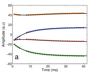
(a) $|\psi\rangle=\left|00\right\rangle$

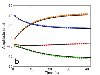
(b) $|\psi\rangle=\left|01\right\rangle$

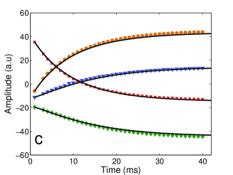
(c) $|\psi\rangle=\left|10\right\rangle$

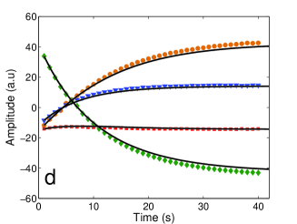
(d) $|\psi\rangle=\left|11\right\rangle$

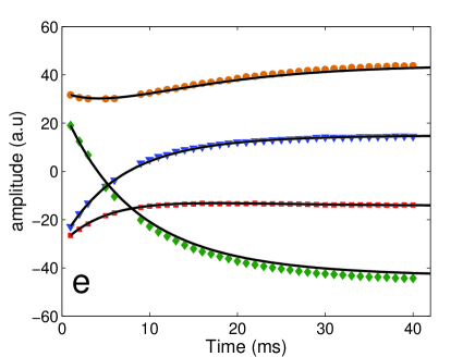
(e) $|\psi\rangle=\frac{1}{\sqrt{2}}(|00\rangle+|11\rangle)$

Fig. 10. Combined experimental data ( $\bullet$-$\rho_{00}$, $\blacktriangledown$-$\rho_{11}$, $\blacksquare$-$\rho_{22}$, $\Diamond$-$\rho_{33}$ ) and the corresponding theoretical prediction (solid lines) obtained from the circuit (5) for various input states. The experimental data were obtained from previous experiments [27].

Fig. 10. Combined experimental data ( $\bullet$-$\rho_{00}$, $\blacktriangledown$-$\rho_{11}$, $\blacksquare$-$\rho_{22}$, $\Diamond$-$\rho_{33}$ ) and the corresponding theoretical prediction (solid lines) obtained from the circuit (5) for various input states. The experimental data were obtained from previous experiments [27].

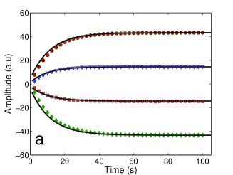
(a) $\bullet$-$\rho_{00}$, $\blacktriangledown$-$\rho_{11}$, $\blacksquare$-$\rho_{22}$, $\Diamond$-$\rho_{33}$.

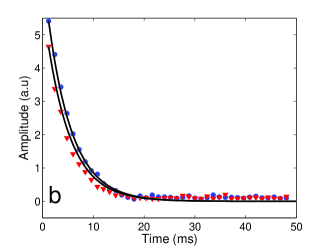
(b) $\bullet$-$\rho_{02}$, $\blacktriangledown$-$\rho_{13}$

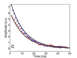
(c) $\bullet$-$\rho_{12}$, $\blacktriangledown$-$\rho_{03}$

Fig. 11. Combined experimental data (symbols) and the corresponding theoretical prediction (solid lines) obtained from the circuit (5) and starting from the state $\frac{1}{2}(|00\rangle+|01\rangle+|10\rangle+|11\rangle)$. The experimental data were obtained from previous experiments [27].

Fig. 11. Combined experimental data (symbols) and the corresponding theoretical prediction (solid lines) obtained from the circuit (5) and starting from the state $\frac{1}{2}(|00\rangle+|01\rangle+|10\rangle+|11\rangle)$. The experimental data were obtained from previous experiments [27].

Acknowledgements

The authors acknowledge the financial support of the Brazilian Science Foundations CAPES, CNPq and FAPESP. We also thank the support of the Brazilian network project National Institute for Quantum Information. AMS would like to acknowledge the government of Ontario - Canada.

References

References

- [1] S. Lloyd (2000), Ultimate physical limits to computation, Nature, 406, pp. 1047-1054.
- [2] S.Lloyd (2002), Computational Capacity of the Universe, Phys. Rev. Lett., 88, pp. 237901-237904.
- [3] K.Maruyama, F.Nori and V.Vedral (2009), The physics of Maxwell’s demon and information, Rev. Mod. Phys., 81, pp.1-23.
- [4] S.Lloyd and Y. J.Ng (2004), Black Holes computers, Sci. Am., 291, pp. 52-62.
- [5] S.D.H.Hsu (2006), Physical limits on information processing, Phys. Lett. B, 641, pp. 99-100.
- [6] G.S.Engel, T.R.Calhoun, E.L.Read, T.-K.Ahn, T.Mancal, Y.-C.Cheng, R.E.Blankenship, and G.R. Fleming (2007), Evidence for wavelike energy transfer throughquantum coherence in photosynthetic systems ,Nature, 446, pp. 782-786.
- [7] I.S. Oliveira, R.S. Sarthour, E.R. deAzevedo, T.J. Bonagamba and J.C.C. Freitas (2007),NMR Quantum information processing., Elsevier (Netherland).
- [8] J.Stolze and D. Suter (2004), Quantum Computing: A Short Course from Theory to Experiment., Wiley-VCH.
- [9] A.M.Souza, A.Magalhães, J.Teles, E.R.deAzevedo, T.J.Bonagamba, I.S.Oliveira, and R.S. Sarthour (2008), NMR analog of Bell’s inequalities violation test, New J. Phys., 10, pp. 0330201-03302010.
- [10] R.J.Nelson, D.Cory and S. Lloyd (2000), Experimental demonstration of Greenberger-Horne-Zeilinger correlations using nuclear magnetic resonance, Phys. Rev. A, 61, pp. 0221061-0221065.
- [11] F.A.Bonk, E.R.deAzevedo, R.S.Sarthour, J.D.Bulnes, J.C.C.Freitas, A.P. Guimarães, I.S. Oliveira and T.J.Bonagamba (2005), Quantum logical operations for spin 3/2 quadrupolar nucleimonitored by quantum state tomography, J. Magn. Reson., 175, pp. 226-234.
- [12] F.A.Bonk, R.S. Sarthour, E.R.deAzevedo, J.D.Bulnes, G.L.Mantovani, J.C.C. Freitas, T.J.Bonagamba, A.P. Guimarães, and I.S. Oliveira (2004),Quantum-state tomography for quadrupole nuclei and its application on a two-qubit system, Phys. Rev. A, 69, pp. 043221-043229.
- [13] A.K.Khitrin and B.M. Fung (2000), Nuclear magnetic resonance quantum logic gates using quadrupolar nuclei, J. Chem. Phys., 112, pp. 6963-6965.
- [14] K.V.R.M. Murali, N. Sinha, T.S. Mahesh, M.H. Levitt, K.V. Ramanathan, and A. Kumar (2002), Quantum-information processing by nuclear magnetic resonance: Experimental implementation of half-adder and subtractor operations using an oriented spin-7/2 system, Phys. Rev. A, 66, pp. 0223131-0223135.
- [15] A. Khitrin, H. Sun and B.M. Fung (2001), Method of multifrequency excitation for creating pseudopure states for NMR quantum computing, Phys. Rev. A, 63, pp. 0203011-0203014.
- [16] T.Gopinath and A. Kumar (2008), Implementation of controlled phase shift gates and Collins version of Deutsch-Jozsa algorithm on a quadrupolar spin-7/2 nucleus using non-adiabatic geometric phases, J. Magn. Reson., 193, pp. 168-176.
- [17] H. Kampermann and W.S. Veeman (2005), Characterization of quantum algorithms by quantum process tomography using quadrupolar spins in solid-state nuclear magnetic resonance, J. Chem. Phys., 63, pp. 2141081-2141086.
- [18] G.Yusa, K.Muraki, K.Takashina, K. Hashimoto and Y. Hirayama (2005), Controlled multiple quantum coherences of nuclear spins in a nanometre-scale device, Nature, 434, pp. 1001-1005.
- [19] M.N.Leuenberger, D.Loss, M. Poggio and D.D. Awschalom (2002), Quantum Information Processing with Large Nuclear Spins in GaAs Semiconductors , Phys. Rev. Lett. 89, pp. 2076011-2076014.
- [20] Y.Kondo, M. Ono, S.Matsuzaka, K.Morita, H.Sanada, Y.Ohno and H.Ohno (2008), Multipulse Operation and Optical Detection of Nuclear Spin Coherence in a GaAs/AlGaAs Quantum Well, Phys. Rev. Lett., 101, pp. 2076011-2076014.
- [21] Y.Hirayama, A.Miranowicz, T.Ota, G.Yusa, K.Muraki, S.Ozdemir and N.Imoto (2006), Nanometre-scale nuclear-spin device for quantum information processing, J.Phys.:Condens. Matter, 18, pp. S885-S900.
- [22] M.A. Nielsen and I.L. Chuang (2000),Quantum Computation and Quantum Information, Cambridge University Press, (Cambridge).
- [23] A. Abragam (1994), Principles of Nuclear Magnetism, Oxford Science Publications, (Oxford).
- [24] P. Gerothanassis and C.G. Tsanaktsidis (1996), Nuclear Electric Quadrupole Relaxation, Concepts Magn. Reson., 8, pp. 63-74.
- [25] R.S.Sarthour, E.R.deAzevedo, F.A.Bonk, E.L.G.Vidoto, T.J.Bonagamba, A.P.Guimarães, J.C.C.Freitas and I.S.Oliveira (2003), Relaxation of coherent states in a two qubit NMR quadrupole system, Phys. Rev. A, 68, pp.0223111-0223117.
- [26] A.G. Redfield (1957), On the Theory of relaxation Processes, IBM J. Res. Dev, 1, pp. 19-31.
- [27] R.Auccaise, J.Teles, R.S.Sarthour, T.J.Bonagamba, I.S.Oliveira, and E.R. deAzevedo (2008), A study of the relaxation dynamics in a quadrupolar NMR system using Quantum state Tomography, J. Magn. Reson. 192, pp. 17-26.
- [28] J.R.C. van der Maarel (1991), Relaxation of spin quantum number S = 3/2 under multiple pulse quadrupolar echoes, J. Chem. Phys., 94, pp. 4765-4775.
- [29] G.Jaccard, S.Wimperis and G.Bodenhausen (1986), Multiple quantum NMR spectroscopy of S = 3/2 spins in isotropic phase: a new probe for multiexponencial relaxation, J. Chem. Phys., 85, pp. 6282-6293.
- [30] A. Al-Qasimi and D.F.V. James (2008), Sudden death of entanglement at finite temperature, Phys. Rev. A, 77, pp. 0121171-0121174.
- [31] K.Radley, L.W. Reeves, and A.S.Tracey (1976), Effect of Counterion Substitution on the Type and Nature of Nematic Lyotropic Phases from Nuclear Magnetic Resonance Studies, J. Chem. Phys., 80, pp. 176-182.
- [32] E.M.Fortunato, M.A.Pravia, N.Boulant, G.Teklemariam, T.F.Havel and D.G.Cory (2002), Multiple quantum NMR spectroscopy of S = 3/2 spins in isotropic phase: a new probe for multiexponencial relaxation, J. Chem. Phys., 116, pp. 7599-7606.
- [33] D.Suter and T.S.Mahesh (2008), Spins as qubits: Quantum information processing by nuclear magnetic resonance, J. Chem. Phys., 128, pp. 0522061-05220614.
- [34] J.Teles, E.R. deAzevedo, R.Auccaise, R.S.Sarthour, I.S.Oliveira and T.J. Bonagamba (2007), Quantum state tomography for quadrupolar nuclei using global rotations of the spin system, J. Chem. Phys. 126, pp. 1545061-1545068.