Widespread nanoflare variability detected with Hinode/XRT in a solar active region

Abstract

It is generally agreed that small impulsive energy bursts called nanoflares are responsible for at least some of the Sun’s hot corona, but whether they are the explanation for most of the multi-million degree plasma has been a matter of ongoing debate. We here present evidence that nanoflares are widespread in an active region observed by the X-Ray Telescope on-board the Hinode mission. The distributions of intensity fluctuations have small but important asymmetries, whether taken from individual pixels, multi-pixel subregions, or the entire active region. Negative fluctuations (corresponding to reduced intensity) are greater in number but weaker in amplitude, so that the median fluctuation is negative compared to a mean of zero. Using MonteCarlo simulations, we show that only part of this asymmetry can be explained by Poisson photon statistics. The remainder is explainable with a tendency for exponentially decreasing intensity, such as would be expected from a cooling plasma produced from a nanoflare. We suggest that nanoflares are a universal heating process within active regions.

1 Introduction

How the outer atmosphere of the Sun, the solar corona, is heated to several million degrees Kelvin is one of the most compelling questions in space science (Klimchuk, 2006). Simple thermal conduction from below is clearly not the answer, since the corona is more than two orders of magnitude hotter than the solar surface. Indeed, whatever mechanism heats the corona must do so in the face of strong energy losses from both downward thermal conduction and radiation.

Soft X-ray and EUV images of the corona reveal many beautiful loop structures—arched magnetic flux tubes filled with plasma. It is generally agreed that warm loops – whose temperature is only about 1 MK, well observed in EUV images – are bundles of unresolved thin strands that are heated by small energy bursts called nanoflares (Parker, 1988; Gomez et al., 1993; Warren et al., 2002; Klimchuk, 2006; Sakamoto et al., 2008). Identifiable warm loops account for only a small fraction of the coronal plasma, however. Most emission has a diffuse appearance, and the question remains as to how this dominant component is heated, especially in the hotter central parts of active regions. Is it also energized by nanoflares, or is the heating more steady? Recent observations have revealed that small amounts of extremely hot plasma are widespread in active regions (Reale et al., 2009) and are consistent with the predictions of theoretical nanoflare models (Klimchuk et al., 2008). This suggests that nanoflare heating may indeed be universal. However, the conclusion is far from certain (Brooks & Warren, 2009). The work reported here sheds new light on this fundamental question.

A magnetic strand that is heated by a nanoflare evolves in a well defined manner. Its light curve (intensity vs. time) has a characteristic shape: the intensity rises quickly as the nanoflare occurs, levels off temporarily, then enters a longer period of exponential decay as the plasma cools (López Fuentes & Klimchuk, 2010). If we could isolate individual strands in real observations, it would be easy to establish whether the heating is impulsive or steady. Unfortunately, this is not the case. The corona is optically thin, so each line of sight represents an integration through a large number overlapping translucent strands. Nonetheless, it may be possible to infer the presence of nanoflares.

Actual light curves exhibit both long and short-term temporal variations. Some of the short-term fluctuation is due to photon statistical noise, but some may be caused by nanoflares. The amplitude of the fluctuations seems to be larger than expected from noise alone (Sakamoto et al., 2008, 2009; Vekstein, 2009). However, this is difficult to determine with confidence, because the precise level of noise depends on the temperature of the plasma, and this is known only approximately in these studies. As we report here for the first time, there is another method for detecting nanoflares from intensity fluctuations that does not depend sensitively on the noise. If heating is impulsive we expect the light curves of individual strands to be asymmetric. The strand is bright for less time than it is faint, and when it is bright it is much brighter than the temporal average. This results in a distribution of intensities that is also very asymmetric. A good measure of the asymmetry is the difference between the median and mean values. This is a generic property of light curves that are dominated by an exponential decay, as is the case with nanoflares. We use this property to demonstrate that nanoflares are occurring throughout a particular active region that we studied in detail. Since the light curve at each pixel in the image set is a composite of many light curves from along the line-of-sight, the asymmetries of the intensity distributions and the differences between the median and mean values are small. We use both statistical analysis and quantitative modeling to show that the differences are nonetheless significant and consistent with widespread nanoflaring in the active region.

In Section 2 we describe the data analysis and results, in Section 3 we interpret the results in the light of Monte Carlo simulations and of loop modeling and in Section 4 the whole scenario is discussed.

2 Data analysis

2.1 The observation and preliminary analysis

The grazing-incidence X-Ray Telescope (XRT) (Golub et al., 2007; Kano et al., 2008; Narukage et al., 2011) on the Hinode spacecraft (Kosugi et al., 2007) detects plasmas in the temperature range $6.1<\log~{}T<7.5$ with 1 arcsec spatial resolution. Active region AR 10923 was observed on 14 November 2006 near the center of the solar disk. It was also studied previously in other ways (Reale et al., 2007, 2009). The observations used for this study were made in the Al_poly filterband starting at 11 UT and lasting $\sim 26$ min. A total of 303 images were taken with a 0.26 s exposure at cadence intervals between 3 and 9 s. No major flare activity or significant change in the morphology occurred during this time. We concentrated on a 256$\times$256 arcsec² field of view and used the standard XRT software to calibrate the data. The images were co-aligned using the jitter information provided with the data.

2.2 Data cleaning

Because we are interested in low level systematic variations that could be indicative of nanoflares, we removed pixels from the dataset that show phenomena which may obscure the effect we are attempting to study. Our analysis is best applied to light curves that are approximately constant or that exhibit only a slow linear trend. We therefore excluded pixels that have a low signal or that show macroscopic variations that might be attributed to cosmic ray hits, microflares or other transient brightenings, or to slow variations due, for instance, to local loop drifts or motions. We discuss each of these possibilities in turn.

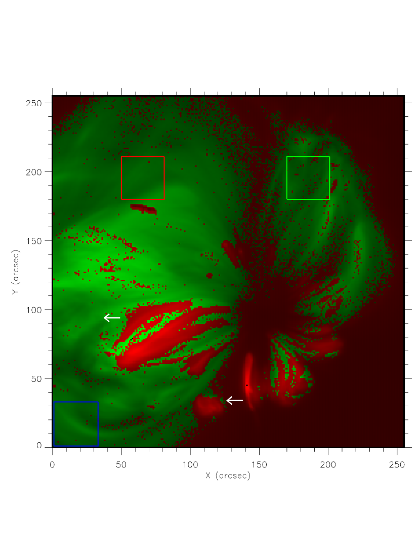
Since we expect the fluctuations that result from episodic heating to be erratic and of very small amplitude, they may be very difficult to distinguish from the noise, so we removed all pixels with an average count rate below $30DN/s$. This is essentially the entire dark area outside of the active region proper. These pixels amount to $\sim 11$% of the total. We removed all pixels affected by bright spikes due to cosmic rays or point-like brightenings. These pixels were identified by the condition that the signal is at least $1.5$ times the spatial median of the immediately surrounding pixels (Sakamoto et al., 2009). They represent $\sim 15\%$ of the total. We also excluded continuous macroscopic events, i.e. large scale events such as microflares. To this aim, we performed a linear fit of the pixel light curve and removed the pixels whose intensity became or exceeded 1.5 times of the bestfit line at any time during the observation. These account for $\sim 10\%$ of the total. Finally, we removed slow intensity variations due to displacement or drift of coronal structures along the line of sight. We used a method based on counting the number of crossings of the bestfit line by the light curve. If the fluctuations of m data points around the linear fit are completely random, the time profile has m-1 possibilities to cross the linear fit, with $0.5$ probability. The “number of crossings” follows a Binomial distribution with a mean of ${(m-1)}/{2}$ and a standard deviation of ${\sqrt{(m-1)}}/{2}$. Assuming that the duration of intrinsic intensity fluctuations is shorter than the observing time ($\sim 26$ min), and the duration of the fluctuations due to loop drifts or motions is comparable with observing time, the number of crossings due to loop motions should be smaller than $\sqrt{(m-1)}/{2}$. We removed all pixels where the number of crossings is smaller than the mean of the binomial distribution ($\sim 7\%$). At the end of the cleaning we are left with about $56\%$ of the total number of pixels as shown in Figure 1.

2.3 Temporal analysis

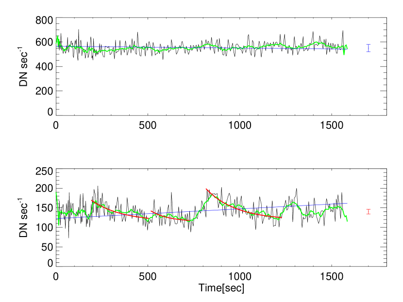
The light curves of the remaining pixels (green in Fig.1) can be fit satisfactorily well with a linear regression. The slopes tend to be very small ($0\pm 0.15$ in $90\%$ of the cases), and there is no preference for increasing or decreasing intensity. Figure 2 shows light curves for two sample pixels with the linear fit in blue and 9-point ($\sim 1$ min) running averages in green. The light curve in the lower panel is one with a highly negative median, and on it we mark three decaying exponentials that fit well the respective data segments and provide good evidence for cooling (see Sections 3.1,4). We measure intensity fluctuations relative to the linear fit according to:

$$dI(x,y,t)=\frac{I(x,y,t)-I_{0}(x,y,t)}{\sigma_{P}(x,y,t)}$$ (1)

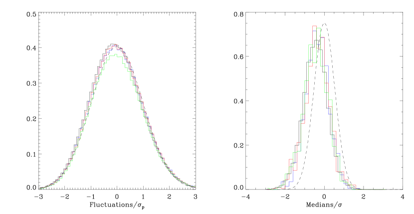
where $I(x,y,t)$ is the count rate (DN/s) at position $[x,y]$ and time $t$, $I_{0}(x,y,t)$ is the value of the linear fit at the same position and time, and $\sigma_{P}(x,y,t)$ is the photon noise estimated as the standard deviation of the pixel light curve with respect to the linear fit, with a small correction to account for the variation of the average count rate with time (described by the linear fit). The distribution of the intensity fluctuations (Fig.3) is not symmetric at either pixel. There is a slight excess of negative fluctuations (fainter than average emission) compared to positive. The mean fluctuation is 0, by definition, but the median fluctuation (normalized to $\sigma_{P}$) is $-0.08\pm 0.07$ in the brighter pixel (upper panel of Fig. 2) and $-0.12\pm 0.07$ in the fainter pixel (lower panel of Fig. 2). The uncertainties in the median values have been rigorously computed according to Hong et al. (2004).

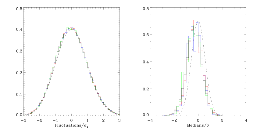
Since the fluctuations of each pixel light curve are normalized, in the same way we can build a distribution with higher statistical significance simply including the fluctuations from more pixels. Figure 4 (left panel) shows the distributions of the three $32\times 32$ pixels sub-regions marked in Figure 1 and of the whole active region. Subtle asymmetries can be detected by eye when compared to the Gaussian distribution shown as a dashed curve for comparison. The right panel in Figure 4 shows the distributions of the median values themselves, computed individually at each pixel. There is a clear preference for the medians to be negative. The median averages (coinciding with the peak of the median distributions, that are highly symmetric) are between $-0.025\pm 0.002$ and $-0.030\pm 0.002$ for the sub-regions and $-0.0258\pm 0.0004$ for the entire active region. Uncertainties are estimated according to Hong et al. (2004). Results for the active region and the selected subregions are listed in Table 1. The fact that the results are similar in the subregions and in the whole active region (and the significance increases) is important because it shows that the effect is widespread and real. Were it due simply to random Gaussian fluctuations (or fluctuations of any random variable that is symmetrically distributed), the magnitude would decrease as more and more pixels are included in the statistics, i.e., the effect would be smaller for the whole active region. Furthermore, if the effect were due entirely to photon noise, which obeys Poisson statistics (see next Section), then increasing the sample size would bring the Poisson distribution closer to a symmetric Gaussian and decrease the difference between the median and the mean (i.e., bring the mean closer to zero). However, the measured median is just as large for the entire active region as it is for the sub-regions.

3 Modeling and interpretation

3.1 MonteCarlo simulations

Photon counting obeys Poisson statistics, and since the Poisson distribution is asymmetric, part of the negative offset of the median values is due to photon noise. We determine how much by performing MonteCarlo simulations to generate synthetic light curves for an appropriate number of pixels.

As a null-hypothesis, we assume that the fluctuations at each pixel are due only to photon noise, i.e., that the intrinsic light curve is flat. To simulate this, we start from an observed emission map obtained by time averaging all the actual images. We then introduce synthetic noise at each pixel using Poisson statistics and having the same average fluctuation amplitude as observed, derived according to Equation 1. In this way we obtain a noisy light curve, with fluctuations Poisson-distributed around the zero-value. We repeat this procedure for all valid pixels, thereby obtaining a datacube of artificial XRT images exactly analogous to the real one. We can then apply the same analysis to the synthetic data. As already mentioned, we obtain asymmetric distributions from the null-hypothesis. For the three subregions marked in Figure 1 we obtain median values between $-0.013\pm 0.002$ and $-0.018\pm 0.002$. These values are incompatible with and significantly lower than those measured from the observational data ($-0.025/-0.030\pm 0.002$). For the whole region we obtain $-0.0164\pm 0.0004$ to be compared to $-0.0258\pm 0.0004$ from the data. Analogously we have computed that for all pixels with an average rate $\geq 800$ and $\geq 1600$ DN/s the median distribution for the whole region is $-0.0096\pm 0.0009$ and $-0.0096\pm 0.0017$, respectively, to be compared with observational data ($-0.0160\pm 0.0009$ and $-0.0136\pm 0.0018$) for the same threshold values respectively.

Our next step is to perturb the intrinsically flat light curves with a sequence of random segments of exponential decays, linked one to the other. We slightly reduce the constant offset so as to maintain the same average DN rate after adding the perturbations, which are all positive. The parameters of the perturbations are the $e$-folding time, $\tau$, the average time interval between two successive perturbations, $dt$, and the amplitude, $A$. The $e$-folding time is fixed for each simulation. The cadence is Poisson-distributed around the average value, because each perturbation is triggered an integer number of frames after the previous one. Since the number of frames is relatively large (tens) the Poisson distribution approaches a Gaussian one. The amplitude is random-uniform between 0.5 and 1.5 of the average value.

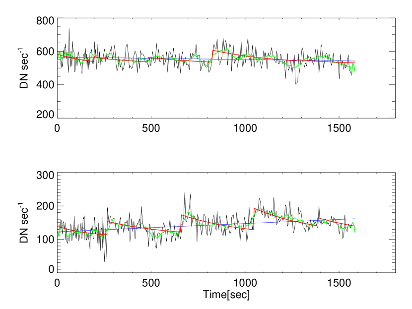
The flat light curve becomes “saw-toothed”, but non-periodic, with exponential descending trends. This new light curve is then randomized according to the pixel average counting statistics, as was done for the constant light curve (Fig.5). Again, we repeat this procedure for all valid pixels to obtain new datacubes, which we analyze as if they were real data.

We perform a sample exploration of the parameter space. In particular, we consider reasonable loop cooling timescales as possible $e$-folding times, i.e. $\tau=180,\;360,\;540\;s$. The larger values more likely for realistic active region loops of length $5-10\times 10^{9}$ cm, according to the loop cooling times ($\tau_{s}$), which are of the order of (Serio et al., 1991):

$$\tau_{s}=4.8\times 10^{-4}\frac{L}{\sqrt{T_{0}}}=120\frac{L_{9}}{\sqrt{T_{0,7}}}$$ (2)

where $L$ ($L_{9}$) is the loop half-length (in units of $10^{9}$ cm) and $T_{0}$ ($T_{0,7}$) is the loop maximum temperature (in units of $10^{7}$ K). To give a significantly negative median, each exponential must be visible uninterrupted for a relatively long time, even more since its amplitude is relatively small with respect to the constant background. Therefore we have set the average time interval between two successive perturbations to a value compatible with the chosen $e$-folding time. We make two different sets of simulations with amplitude A = $30$ and $60\;DN/s$.

The results of the simulations are listed in Tables 2 and 3. The median values from the simulations approach those obtained from the data for all values of $\tau$, for $A=60$ DN/s, and for time intervals of the order or larger than $\tau$ (Figures 4 and 6). The best match with data results is obtained with $A=60$ DN/s, $\tau=360\;s$ and $dt=360\;s$.

It is worth commenting further on the distribution of median values obtained from the individual pixels (Figures 4 and 6, right panels). As we have discussed, a negative median is indicative of exponentially decreasing intensity and cooling plasma (and also Poisson photon statistics to some degree). However, a sizable fraction of the observed median values are positive. Without the benefit of our simulations, we might conclude that these pixels do not have cooling plasma. The good agreement between the observed (Fig.4, right panel) and simulated (Fig.6, right panel) distributions, both in terms of the centroid offset and the width, shows that the observations are in fact consistent with all of the pixels having cooling plasma. Positive median values occur when photon statistics mask the relative weak signal of the exponentially decreasing intensity.

3.2 Loop hydrodynamic modeling

In a possible scenario, a coronal loop consists of many independent strands, each ignited by a heat pulse that we call a nanoflare. The evolution of the plasma confined in a single strand driven by a heat pulse has been described in the past by means of time-dependent hydrodynamic loop models (Nagai, 1980; Peres et al., 1982; Cheng et al., 1983; Fisher et al., 1985; MacNeice, 1986). The light curve in Figure 7 is synthesized in the Hinode/XRT Al_poly filterband from the results of a hydrodynamic model of a nanoflaring strand (Guarrasi et al., 2010). This hydrodynamic simulation has been used successfully to explain totally different observational results, which indicates that the parameters are realistic. The strand half-length is $3\times 10^{9}$ cm. The heat pulse of the single strand is a top-hat function in time, the high state lasting $60\;s$, and in space it is uniformly distributed along the strand. Its intensity is 0.38 erg cm^-3 s^-1 and brings the strand to a maximum temperature $\log T\approx 7$. The total energy injected in the strand is therefore $\approx 1.4\times 10^{11}$ erg cm^-2 to be multiplied by the strand cross-section area. The loop hydrodynamic simulations are one-dimensional and in the synthesis of the loop emission the cross-section area is a free parameter. We have chosen the cross-section area so as to have an emission peak of 60 DN/s, a realistic value suggested by the MonteCarlo simulations described above. The light curve is characterized by a steep rise phase, a short plateau and a much longer decay phase, which can be well approximated by a decreasing exponential (Figure 7). For this particular model strand (it depends on the strand half-length, see Eq. 2), the best-fit $e$-folding time is $\sim 300$ s. We verified that the median intensity (7.0 DN/s) is much smaller than (less than half of) the mean intensity (16.6 DN/s).

4 Discussion

We find evidence that the light curves in each pixel of an active region have systematic features: the distribution of intensity fluctuations is asymmetric and the median value is less than the mean. The effect is confirmed and even at higher level of significance when summed over larger and larger parts of the region, and therefore widespread and real.

We have also shown that part of the negative offset of the median values is due to photon noise. We determine how much by performing MonteCarlo simulations to generate synthetic light curves. Comparing the value of the median for the entire region in Table 1 with the value of the median for the simulations with Poisson noise only (null hypothesis, $A=0$, $threshold=30$ in Table 2) we see that the Poisson noise accounts only for the $\sim 60$% of the negative shift of the median. The significance of the remainder is at the $5\sigma$ level for the subregions and $25\sigma$ level for the active region!

We also perform simulations meant to represent cooling plasma by randomly adding pieces of exponential decays onto the constant background intensity. Photon noise is included as explained above. The resulting light curves (see Figure 5) look similar to those in Figure 2. The distributions of the intensity fluctuations agree well with observations, with median values that have a similar negative offset. As an aside, the parameters of the simulations lead to realistic constraints about the loop substructuring (see the Appendix). We roughly estimate a possible strand diameter around $10^{7}$ cm, i.e. a fraction of arcsec, not far from the resolution of the current instruments. Probably these are the most significant nanoflare events, the high tail of a distribution. The bulk of the events may occur with higher frequency and in finer strands.

We remark that our analysis is entirely independent of filter calibration and highly model-independent. The data error is in principle dependent on the emitted spectrum and therefore on the plasma temperature and filter calibration, but we have estimated it directly from the noise of the light curves. The model we use in Monte Carlo simulations is very simple and has a minimal set of free parameters.

Previous attempts to determine the nature of coronal heating outside of isolated warm loops have been inconclusive (Brooks & Warren, 2009; Tripathi et al., 2011). Our study provides strong evidence for widespread cooling plasma in active region AR 10923. This suggests heating that is impulsive and definitively excludes steady heating, which in turn suggests that nanoflares play a universal role in active regions. We favor nanoflares occurring within the corona, but we do not exclude that our observations may also be consistent with the impulsive injection of hot plasma from below, as has recently been suggested (De Pontieu et al., 2011).

Appendix A Loop substructuring

We can make simple estimates of some characteristics implied by the parameters constrained with MonteCarlo simulations. Let us assume that the events that we resolve are able to heat an active region loop, that an event observed in a pixel heats a whole loop strand, that the intensity of each event is able to bring the loop to a temperature of 10 MK, with an average temperature of 3 MK, and that the loop has a total length of $2L=5\times 10^{9}$ cm.

From MonteCarlo simulations, we find that an appropriate average event cadence interval is:

$$dt\geq 360~{}~{}s$$

For an observation duration:

$$\Delta t=1600~{}~{}s$$

the number of events per pixel is:

$$dn\approx\frac{\Delta t}{dt}\leq 4$$

If we assume an average loop half-length ($10^{9}$ cm):

$$L_{9}\approx 2.5$$

and a loop diameter (typically $10$% of the loop length):

$$D\approx 0.1\times 2L\approx 0.5\times 10^{9}{\rm cm}\approx 7~{}~{}{\rm pix}$$

The number of events in the loop is:

$$n\approx dn\times D\leq 30$$

From loop scaling laws (Rosner et al., 1978) , we estimate the equilibrium pressure corresponding to the maximum temperature (MK) $T_{max,6}=10$, possibly due to a heat pulse:

$$p\approx 0.3\frac{T_{0,6}^{3}}{L_{9}}\sim 100~{}{\rm dyne~{}cm^{-2}}$$

From this we roughly estimate the pulse heating rate per unit volume in units of $10^{-3}{\rm erg~{}cm^{-3}~{}s^{-1}}$ to bring a strand to a temperature of 10 MK:

$$H_{-3}=3p^{7/6}~{}L_{9}^{-5/6}\sim 300$$

and the pulse energy flux over the whole loop:

$$F=H\times 2~{}L\sim 0.3\times 5\times 10^{9}\sim 1.5\times 10^{9}~{}~{}~{}{\rm erg~{}cm^{-2}~{}s^{-1}}$$

The energy released by the nanoflare in the loop is then:

$$E_{n}=F~{}n~{}t_{n}~{}dA_{n}\leq 1.5\times 10^{9}\times 30t_{n}~{}dA_{n}\approx 4\times 10^{10}t_{n}~{}dA_{n}$$

where $t_{n}$ is the nanoflare duration and $dA_{n}$ is strand cross-section area.

Let’s now consider the average loop conditions. For a loop cross-section of:

$$A=\pi~{}R^{2}\sim\pi 6\times 10^{16}\sim 2\times 10^{17}~{}~{}{\rm cm}^{2}$$

and an average loop heating rate per unit volume for steady state ($T_{max,6}=3$):

$$\langle H\rangle\sim 0.002~{}~{}{\rm erg~{}cm^{-3}~{}s^{-1}}$$

The loop total thermal energy in the observation can be estimated as:

$$E_{L}\approx\langle H\rangle~{}2~{}L~{}A~{}\Delta t\approx 0.002\times 2\times 2.5\times 10^{9}\times 2\times 10^{17}\times 1600\approx 3\times 10^{27}~{}~{}~{}{\rm erg}$$

By equating $E_{n}\approx E_{L}$, we obtain:

$$t_{n}\frac{dA_{n}}{A}\geq\frac{3\times 10^{27}}{4\times 10^{10}\times 2\times 10^{17}}\approx 0.5$$

So the product of the nanoflare duration (in s) and the fractional strand area is of the order of 1. For instance, if the nanoflare lasts 60 s we fill the loop with about 120 strands. The implication would be that the strand diameter is more than $10^{7}$ cm, but we warn that this is a crude estimate, based on scaling laws that hold only roughly out of equilibrium.

Table 1: Active Region Analysis results

Data	Threshold 30	Threshold 800	Threshold 1600
Region	-0.0258$\pm$0.0004	-0.0160$\pm$0.0009	-0.0136$\pm$0.0018
Sub-reg 1	-0.025$\pm$0.002	$\cdots$	$\cdots$
Sub-reg 2	-0.026$\pm$0.002	$\cdots$	$\cdots$
Sub-reg 3	-0.030$\pm$0.002	$\cdots$	$\cdots$

Note. — Table 1 shows the values of the median averages, with errors, for the entire active region, and for the selected subregions (Fig.1). The listed values for the entire active region are obtained analyzing only pixels with intensity over three different threshold values.

Table 2: MonteCarlo Simulations results

$A^{\;1}$	$dt^{\;2}$	$\tau^{\;2}$	$Thr=30^{\;1}$	Thr=800	Thr=1600
0	0	0	-0.0164$\pm$0.0004	-0.0096$\pm$0.0009	-0.0096$\pm$0.0017
30${}^{\;\;}$	360	360	-0.0184$\pm$0.0004	-0.0105$\pm$0.0005	-0.0087$\pm$0.0017
30${}^{\;\;}$	540	360	-0.0189$\pm$0.0004	-0.0099$\pm$0.0009	-0.0086$\pm$0.0018
60${}^{\;\;}$	360	180	-0.0322$\pm$0.0004	-0.0136$\pm$0.0008	-0.0109$\pm$0.0017
60 3	360	360	-0.0253$\pm$0.0004	-0.0112$\pm$0.0009	-0.0070$\pm$0.0017
60${}^{\;\;}$	360	540	-0.0228$\pm$0.0004	-0.0103$\pm$0.0009	-0.0063$\pm$0.0018
60${}^{\;\;}$	540	360	-0.0283$\pm$0.0004	-0.0124$\pm$0.0008	-0.0087$\pm$0.0017

Note. — Table 2 shows the simulated values of averaged medians, with errors, for nanoflares heated active region. The cadence is Poisson-distributed around the average value, the amplitude is random-uniform between 0.5 and 1.5 the average value, A. A $=0$ is the null-hypothesis (no perturbation).

Table 3: MonteCarlo Simulations results for Sub-regions

A	dt	Sub-reg 1	Sub-reg 2	Sub-reg 3
0	0	-0.016$\pm$0.002	-0.013$\pm$0.002	-0.018$\pm$0.002
30	360	-0.018$\pm$0.002	-0.018$\pm$0.002	-0.018$\pm$0.002
30	540	-0.021$\pm$0.002	-0.017$\pm$0.002	-0.020$\pm$0.002
60	360	-0.021$\pm$0.002	-0.021$\pm$0.002	-0.024$\pm$0.002
60	540	-0.024$\pm$0.002	-0.024$\pm$0.002	-0.028$\pm$0.002

Note. — Table 3 shows the simulated values of averaged medians, with errors, for selected sub-regions (Fig.1) obtained from MonteCarlo simulations, with units as in Tab.2.

Figure 1: Active region AR 10923 observed with the Hinode/XRT Al_poly filter on 14 November 2006 at 11 UT. We distinguish between pixels accepted (green) and rejected (red) for the analysis. The color scales are powers of the intensity (0.5 and 0.1 for green and red respectively), with maxima of 57 DN/s and 1171 DN/s respectively. We mark three subregions (frames) which are analyzed specifically. We show in Figure 2 the light curves of two pixels (indicated by the arrows).

Figure 2: Light curves of two selected pixels indicated in Figure 1. Linear fits are shown in blue; 9-point ($\sim 1$ min) running averages are shown in green; in the lower panel we show sample decaying exponentials (red) that fit well some data segments.

Figure 3: Distributions of the fluctuations of the light curves with respect to the linear fit in the two selected pixels of Figure 1 and 2. The fluctuations amplitude distributions are normalized to the Poisson noise. A Gaussian centered on zero and having unit width is plotted for reference (dashed line).

Figure 4: The left panel shows the combined distributions of fluctuations for the pixels in three selected regions (color coded to match the boxes in Figure 1) and in the whole active region (black histogram). The right panel shows the distributions of the median fluctuation values computed individually at each pixel. Fluctuations are normalized to the Poisson noise (left), and medians are normalized to their standard deviation (right). Gaussians centered on zero and having unit width are plotted for reference (dashed line).

Figure 5: Light curves of two pixels obtained from Monte Carlo simulations adding trains of exponentials (red). The linear fits are marked (blue lines); 9-point ($\sim 1$ min) running averages are shown (green).

Figure 6: Identical to Figure 4 but obtained with the MonteCarlo simulation with: $A=60$ DN/s, $\tau=360$ s, and $dt=360$ s.

Figure 7: Light curve in the XRT Al_poly filterband obtained from a hydrodynamic simulation of the plasma confined in a loop strand ignited by a heat pulse (nanoflare). The heat pulse lasts 60 s and brings the strand to a maximum temperature $\log T\approx 7$. Most of the decay is well described by an exponential with an $e$-folding time $\tau\approx 300$ s (dashed line). Solid and dashed horizontal lines show the mean and median intensity, respectively.

References

- Brooks & Warren (2009) Brooks, D. H., & Warren, H. P. 2009, ApJ, 703, L10
- Cheng et al. (1983) Cheng, C., Oran, E. S., Doschek, G. A., Boris, J. P., & Mariska, J. T. 1983, ApJ, 265, 1090
- De Pontieu et al. (2011) De Pontieu, B. et al. 2011, Science, 331, 55
- Fisher et al. (1985) Fisher, G. H., Canfield, R. C., & McClymont, A. N. 1985, ApJ, 289, 414
- Golub et al. (2007) Golub, L. et al. 2007, Sol. Phys., 243, 63
- Gomez et al. (1993) Gomez, D. O., Martens, P. C. H., & Golub, L. 1993, ApJ, 405, 767
- Guarrasi et al. (2010) Guarrasi, M., Reale, F., & Peres, G. 2010, ApJ, 719, 576
- Hong et al. (2004) Hong, J., Schlegel, E. M., & Grindlay, J. E. 2004, ApJ, 614, 508
- Kano et al. (2008) Kano, R. et al. 2008, Sol. Phys., 249, 263
- Klimchuk (2006) Klimchuk, J. A. 2006, Sol. Phys., 234, 41
- Klimchuk et al. (2008) Klimchuk, J. A., Patsourakos, S., & Cargill, P. J. 2008, ApJ, 682, 1351
- Kosugi et al. (2007) Kosugi, T. et al. 2007, Sol. Phys., 243, 3
- López Fuentes & Klimchuk (2010) López Fuentes, M. C., & Klimchuk, J. A. 2010, ApJ, 719, 591
- MacNeice (1986) MacNeice, P. 1986, Sol. Phys., 103, 47
- Nagai (1980) Nagai, F. 1980, Sol. Phys., 68, 351
- Narukage et al. (2011) Narukage, N. et al. 2011, Sol. Phys., 269, 169
- Parker (1988) Parker, E. N. 1988, ApJ, 330, 474
- Peres et al. (1982) Peres, G., Serio, S., Vaiana, G. S., & Rosner, R. 1982, ApJ, 252, 791
- Reale et al. (2007) Reale, F. et al. 2007, Science, 318, 1582
- Reale et al. (2009) Reale, F., Testa, P., Klimchuk, J. A., & Parenti, S. 2009, ApJ, 698, 756
- Rosner et al. (1978) Rosner, R., Tucker, W. H., & Vaiana, G. S. 1978, ApJ, 220, 643
- Sakamoto et al. (2008) Sakamoto, Y., Tsuneta, S., & Vekstein, G. 2008, ApJ, 689, 1421
- Sakamoto et al. (2009) —. 2009, ApJ, 703, 2118
- Serio et al. (1991) Serio, S., Reale, F., Jakimiec, J., Sylwester, B., & Sylwester, J. 1991, A&A, 241, 197
- Tripathi et al. (2011) Tripathi, D.,Mason, H. E., & Klimchuk, J. A. 2011, ApJ, in press
- Vekstein (2009) Vekstein, G. 2009, A&A, 499, L5
- Warren et al. (2002) Warren, H. P., Winebarger, A. R., & Hamilton, P. S. 2002, ApJ, 579, L41