Impact of heterogenous prior beliefs and disclosed insider trades thanks: For useful discussions, we thank Deqing Zhou and Bowen Shi. We also would like to thank Jiaan Yan, Jianming Xia and other seminar participants at the Institute of Applied Mathematics, Academy of Mathematics and Systems Science, Chinese Academy of Sciences. The first named author is grateful for financial support for National Natural Science Foundation of China (No.10721101) and China’s National 973 Project (No.2006CB805900). The second author also would like to thank Hengfu Zou, Zhixiang Zhang and other seminar participants at Central University of Finance and Economics.

Fuzhou Gong1  Hong Liu2,3
1 Institute of Applied Mathematics, Academy of Mathematics and Systems Science,
Chinese Academy of Sciences, Beijing, 100190, P.R. China.
2MOE Key Laboratory of Applied Statistics, School of Mathematics and Statistics,
Northeast Normal University, Changchun, 130024, P.R. China
3China Economics and Management Academy, and CIAS,
Central University of Finance and Economics, Beijing, 100081, P.R. China
Corresponding author. E-mail: mathhongliu@gmail.com, liuh653@nenu.edu.cn.
Abstract

In this paper, we present a multi-period trading model by assuming that traders face not only asymmetric information but also heterogenous prior beliefs, under the requirement that the insider publicly disclose his stock trades after the fact. We show that there is an equilibrium in which the irrational insider camouflages his trades with a noise component so that his private information is revealed slowly and linearly whenever he is overconfident or underconfident. We also investigate the relationship between the heterogeneous beliefs and the trade intensity in the presence of trade disclosure, and show that the weights on asymmetric information and heterogeneous prior beliefs are opposite in sign and they change alternatively in the next period. Under the requirement of disclosure, the irrational insider trades more aggressively and leads to smaller market depth. Moreover, the co-existence of “public disclosure requirement” and “heterogeneous prior beliefs” leads to the fluctuant multi-period expected profits and a larger total expected trading volume which is positively related to the degree of heterogeneity. More importantly, even public disclosure may lead to negative profits of the irrational insider’s in some periods, inside trading remains profitable from the whole trading period.

Keywords. public disclosure; asymmetric information; insider trading; price discovery; heterogeneous prior beliefs.

JEL subject classifications: G12; G14

1 Introduction

Anybody, who has a casual look at the security or stock markets, would be amazed by the fluctuation features of financial markets, such as the fluctuation of the trading volume, the price and the short-term aggressive trading. But these fascinating features have rarely been studied in theoretical finance, perhaps for the reason that they seem close to the irrational behavior of traders and can not be explained in the rational expectations. In this paper, we try to study these fascinating features of the market and address the implications on financial market of irrational behavior, by developing a trading model to characterize the optimal behavior of an irrational insider who possesses long-lived private information about the fundamental value of a security under mandatory disclosure requirements.

In his pioneering and insightful paper, Kyle (1985) introduces a dynamic model of insider trading where an insider receives only one signal and the fundamental asset value does not change over time. Through trade, the insider progressively releases his private information to the market as he exploits his informational advantage. Kyle (1985) also points out that liquidity trading provides camouflage which conceals informed trading such that the informed trading is swamped by liquidity trading. Based on Kyle (1985), Huddart, Hughes and Levine (2001) consider the case of the same insider under disclosure requirement as mandated by US securities laws. The ex-post disclosure of the insider’s trades changes the equilibirum strategy of the insider, given that market makers can infer information from the insider’s previous trade before the next round of trading. Huddart, Hughes and Levine (2001) find that public disclosure of the insider’s traders nevertheless accelerates the price discovery process and lowers trading costs by comparison to the case with no disclosure requirement. Zhang (2004) extends Huddart, Hughes and Levine (2001) by incorporating the condition that the monopoly insider is risk-averse, and he finds that under disclosure requirements, the risk-averse insider is more concerned about the risk of sub-optimally revealing his information by mandatory disclosure and his private information is revealed slowly. Also, Zhang (2008) analyzes a dynamic market where outsiders share part of the information about a security with a corporate insider and update their incomplete information by learning from disclosed insider trades. Recently, Gong and Liu (2011) study the optimal behaviors of competitive insiders and their influences to the market under disclosure requirements. All the papers mentioned above have the assumption that the insider is rational. An interesting question is what the behavior of an irrational insider behavior under mandatory disclosure requirements.

In the past few years, lots of literatures have studied the behaviors of irrational traders and their influences to the market. Odean (1998) presents three different markets structures, two of which examine price-taking overconfident informed traders, and one which looks as Kyle (1985)’s setting. His results depend a lot on the specific assumptions about risk preferences of agents and competition. Benos (1998) explicitly models investor behavior in financial markets allowing for traits linked to a notion of imperfect rationality. He studies an extreme form of posterior over confidence where some risk neutral investors overestimate the precision of their private information. In addition, Kyle and Wang (1997) and Wang (1997) consider the case of heterogeneous prior beliefs. The former considers heterogeneous prior beliefs in their study of the survival of irrational traders in a duopoly context while the later examines the implication of overconfidence for delegated fund management in both learning and evolutionary game models. Harris and Raviv (1993) and Wang (1998) use heterogeneous prior beliefs to explain the enormity of volume traded each day. Specifically, Wang (1998) extends the model of Kyle (1985) by incorporating heterogeneous prior beliefs. He finds that in equilibrium, the informed trader, facing both asymmetric information and heterogeneous prior beliefs, smoothes out his trading on asymmetric information gradually over time, but concentrates his entire trading on heterogeneous beliefs toward the last few periods. Since under US securities laws insiders associated with a firm must report to the Securities and Exchange Commission trades they make in the stock of that firm, we try to study the optimal behaviors of an irrational insider, and address its impact to the market under the mandatory disclosure requirements in this paper, using the framework of Kyle (1985).

Kyle (1985)’s model has been widely used to analyze financial market microstructure and the value of information. For example, Holden and Subrahmanyan (1992) and Foster and Viswanathan (1996) consider a market with multiple the competing insiders, and they show that competition among insiders accelerates the release of their private information. Back (1992) formalizes and extends the model by showing the existence of a unique equilibrium beyond the Gaussian-linear framework. Remarkable, when the asset value has a log-normal distribution, the price process becomes a geometric Brownian motion as is usually assumed in finance. Holden and Subrahmanyan (1994) assume the single informed trader is risk-averse. They show that both monopolistic and competing informed traders choose to exploit rents rapidly, causing market depth to be low in the initial periods and high in later periods and causing information to be revealed rapidly, unlike in the case of a risk-neutral monopolist considered by Kyle (1985). Gong and Zhou (2010) improve the Kyle (1985) model by loosing the assumption of constant pricing rule and give a new framework to analysis the insider’s behavior.111We will consider this problem using the new framework in other papers, and the purpose of this paper is to analysis the impact of heterogenous prior beliefs and disclosed insider trades to the market using the framework of Kyle (1985) so as to compare with the modified model. Also, Fishman and Hagerty (1992), Luo (2001), Rochet and Vila (1994), and Jain and Mirman (1999) e.t. have used variance of Kyle’s model to analyze and to explain real financial phenomena.

We consider a model in which traders face both asymmetric information and heterogeneous prior beliefs, with the requirement that the insider publicly disclose his stock trades after the fact. Heterogeneity arises because traders have different distribution assumptions about an informed trader’s private signal, that is to say traders agree to disagree with the precision of the signal. Using the same description as Wang (1998), a trader is overconfident if his distribution of the signal is too tight and underconfident if it is too loose.

We give the existence and the uniqueness of the insider’s equilibrium trading strategy in a multi-period rational expectation framework and give the analysis of the equilibrium. In equilibrium, the “trade public disclosure” and “heterogeneous prior beliefs” have great effects on the insider’s trading intensity, the market depth and the effectiveness of the price.

We obtain many new and interesting results on market characteristics and traders’ strategies. First, under disclosure requirement, the adverse selection decreases when there is an irrational informed trader participating in the market, and the descending range is positive related to the degree of heterogeneity. Since the insider trades more aggressive than he should rationally do, he submits larger orders. The market makers, realizing that the insider is irrational and aggressive behavior, increase market depth. While market makers decrease the market depth if there is no public disclosure requirements, even though the insider is irrational. That is to say, “public disclosure” leads to smaller market depth.

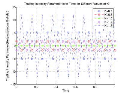
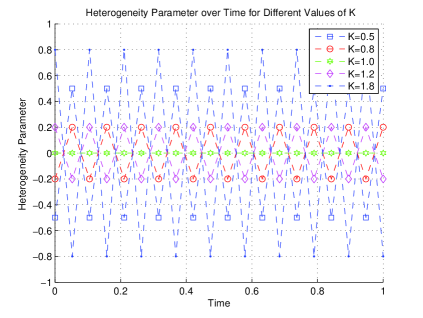
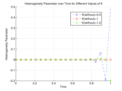
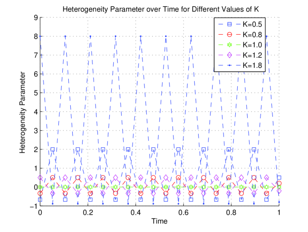
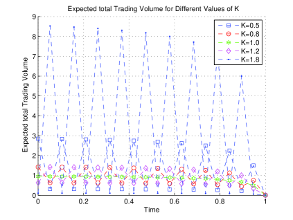
Also, under the disclosure requirement, the irrational insider’s private information is revealed slowly and linearly, for any degree of his heterogeneity. That is to say, under the public disclosure requirement, “heterogeneous beliefs” has no effect on the speed of revelation of information. While “heterogeneous beliefs” has great impacts on the trading behavior of irrational insiders and market structure. In particular, under the disclosure requirement, the insider dissembles his information by adding a random component to his trades in every round except the last one. Despite this, our analysis shows that the information is reflected more rapidly in price with disclosure of insider trades than without. An interesting finding is that when the insider is overconfident or underconfident, the trading intensity of the insider, the heterogeneity parameter and the expected profits all fluctuate greatly during all early auctions. We reveal the relationship between the heterogeneity and the trade intensity in the presence of information disclosure, which agrees with our intuition in the financial market. That is to say, if the underconfident insider puts a positive weight on asymmetric information this period, then he puts a negative weight on heterogeneous prior beliefs this period, and the case is inverse in the next period. We also show that the co-existence of public disclosure and heterogeneous prior beliefs leads to large and fluctuated trading volume and the fluctuation is positively related to the degree of the insider’s heterogeneity.

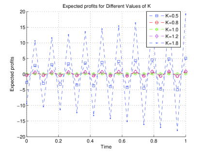
More importantly, the irrational insider’s profits of some trading rounds may be negative under the mandatory disclosure requirement. The expected profits fluctuate during all auctions, and the fluctuation which is positive related to the degree of heterogeneity is small at the early auctions and becomes larger as the trading goes by. Moreover, even though the irrational insider may get negative profits in some periods, he trades to make sure the profit of the last period and the whole trading profit are all positive.

This paper is structured as follows. In Section 222 we introduce the model and in Section 333 we make an analysis and give the two-period equilibrium of the models with and without disclosure of insider trades, respectively. In Section 444, we give the unique linear Nash equilibrium in multi-period framework and give the analysis of the equilibrium. Finally, the appendix contains the proof of some necessary propositions.

2 The model

We conform to the notation of Kyle (1985). A single risky asset with a terminal value v~~𝑣\tilde{v}, which is normally distributed with mean p0subscript𝑝0p_{0} and variance Σ0subscriptΣ0\Sigma_{0}, is traded in an N𝑁N-period sequential auction market among three kinds of risk-neutral traders: a monopolistic informed trader, noise traders and market makers. The monopolistic informed trader has a unique access to a private signal s~\tilde{s}* about v~~𝑣\tilde{v}. All market makers and the insider agree that the signal s~\tilde{s}* is a scalar multiple of the terminal value v~~𝑣\tilde{v}, but they disagree concerning the right scale, that is to say, the informed trader thinks s~=c1v~\tilde{s}*=c_{1}\tilde{v} while the market makers think s~=c2v~\tilde{s}*=c_{2}\tilde{v} , where c1subscript𝑐1c_{1} and c2subscript𝑐2c_{2} are different positive constants. If we consider a normalized signal s~=s~c2~𝑠superscript~𝑠subscript𝑐2\tilde{s}=\frac{\tilde{s}^{*}}{c_{2}}, using the same analysis as Wang (1998) we know that each trader’s heterogeneous prior belief is characterized completely by a parameter K𝐾K, where K=c2/c1𝐾subscript𝑐2subscript𝑐1K=c_{2}/c_{1} is a positive constant. Then the informed trader thinks s~=v~/K~𝑠~𝑣𝐾\tilde{s}=\tilde{v}/K while the market makers think s~=v~~𝑠~𝑣\tilde{s}=\tilde{v}. If we consider the market maker’s beliefs (i.e., K=1𝐾1K=1) as the benchmark case, then the informed trader is “overconfident” if K>1𝐾1K>1 and “underconfident” if 0<K<10𝐾10<K<1. The noise traders (uninformed liquidity traders) trade randomly; and market makers set prices efficiently in the semi-strong form sense, conditional on the total quantities traded by the informed trader and noise traders, but not each of them. We also assume that there is no discount across periods, i.e., the interest rate is normalized to zero. This market model has some game-theoretic features. We can view it as a game played by the insider and the market makers: the insider attempts to hide his private information and make the best use of his information to maximize his profit; the market makers attempt to learn the private information from the order and set prices as efficiently as possible in order to rule out the profit opportunities of the insider.

Let x~nsubscript~𝑥𝑛\tilde{x}_{n} denote the market order submitted by the informed trader at the n𝑛n-th auction, conditional on his information, and let μ~nsubscript~𝜇𝑛\tilde{\mu}_{n} denote the random quantity traded by noise traders at the n𝑛n-th auction. We assume that μ~nsubscript~𝜇𝑛\tilde{\mu}_{n} is normally distributed with zero mean and variance σμ2,superscriptsubscript𝜎𝜇2\sigma_{\mu}^{2}, n=1,2,,N,𝑛12𝑁n=1,2,\cdots,N, and μ~1,μ~2,,μ~N,v~subscript~𝜇1subscript~𝜇2subscript~𝜇𝑁~𝑣\tilde{\mu}_{1},\tilde{\mu}_{2},\cdots,\tilde{\mu}_{N},\tilde{v} are mutually independent. So the total trading volume, denoted by y~nsubscript~𝑦𝑛\tilde{y}_{n}, is given by y~n=x~n+μ~n.subscript~𝑦𝑛subscript~𝑥𝑛subscript~𝜇𝑛\tilde{y}_{n}=\tilde{x}_{n}+\tilde{\mu}_{n}. The market makers set price p~nsubscript~𝑝𝑛\tilde{p}_{n} in semi-strong form sense based on his information y~1,y~2,,y~nsubscript~𝑦1subscript~𝑦2subscript~𝑦𝑛\tilde{y}_{1},\tilde{y}_{2},\cdots,\tilde{y}_{n} at the n𝑛n-th auction. Denote by EK[]subscript𝐸𝐾delimited-[]E_{K}[\cdots] and E1[]subscript𝐸1delimited-[]E_{1}[\cdots] the expectation operators of the informed trader and the market makers, respectively. Then p~n=E1[v~|y~1,,y~n]subscript~𝑝𝑛subscript𝐸1delimited-[]conditional~𝑣subscript~𝑦1subscript~𝑦𝑛\tilde{p}_{n}=E_{1}[\tilde{v}|\tilde{y}_{1},\cdots,\tilde{y}_{n}], n=1,2,,N𝑛12𝑁n=1,2,\cdots,N.

Let π~nsubscript~𝜋𝑛\tilde{\pi}_{n} be the profit which accrues to the informed trader from the n𝑛n-th auction on, i.e., for n=1,2,N,𝑛12𝑁n=1,2\cdots,N, π~n=k=nN(v~p~k)x~ksubscript~𝜋𝑛superscriptsubscript𝑘𝑛𝑁~𝑣subscript~𝑝𝑘subscript~𝑥𝑘\tilde{\pi}_{n}=\sum_{k=n}^{N}(\tilde{v}-\tilde{p}_{k})\tilde{x}_{k}. At each auction the informed trader maximizes his total expected profits of the current and the remaining rounds of trading conditional on his information, i.e.,

maxxEK[π~n|s~=s,p~1=p1,,p~n=pn],forn=1,2,,N.formulae-sequencesubscript𝑥subscript𝐸𝐾delimited-[]formulae-sequenceconditionalsubscript~𝜋𝑛~𝑠𝑠formulae-sequencesubscript~𝑝1subscript𝑝1subscript~𝑝𝑛subscript𝑝𝑛𝑓𝑜𝑟𝑛12𝑁\max_{x}E_{K}[\tilde{\pi}_{n}|\tilde{s}=s,\tilde{p}_{1}=p_{1},\cdots,\tilde{p}_{n}=p_{n}],~{}~{}~{}~{}for~{}~{}~{}n=1,2,\cdots,N.

The equilibrium conditions are that the competition between market makers drives their expected profits to zero conditional on the order flow and the fact that the informed trader selects the optimal strategy conditional on his correct conjectures and his information at each auction. Following the convention in the existing literature, an equilibrium is said to be linear if the pricing rule is an affine function of the order flow. We will give the definition of equilibrium of two-period and N-period in the following sections, respectively.

3 Analysis

3.1 Two-period model without public disclosure of insider trades

In order to get a benchmark against which to compare an equilibrium for the case where the insider’s trade in the first period is publicly disclosed on completion of trading in that period, we first give the two-period equilibrium of the model without public disclosure of insider trades.

The proposition below is based on a special case of Theorem 111 of Wang (1998).

Proposition 3.1.

Given no public disclosure of insider trades, for 0<K<2,0𝐾20<K<2,222Just as the analysis in Wang (1998), the inequality condition 0<K<20𝐾20<K<2 means that if a rational informed trader thinks a risky asset is worth 100100100, then an irrational informed trader’s subjective value cannot be less than 00 or more than 200200200 for the equilibrium to exist. a subgame perfect linear equilibrium exists. In this equilibrium there are constants βn,θn,λn,γn,αn,ωn,ϕn,δnsubscript𝛽𝑛subscript𝜃𝑛subscript𝜆𝑛subscript𝛾𝑛subscript𝛼𝑛subscript𝜔𝑛subscriptitalic-ϕ𝑛subscript𝛿𝑛\beta_{n},\theta_{n},\lambda_{n},\gamma_{n},\alpha_{n},\omega_{n},\phi_{n},\delta_{n} and Σn(n=1,2)subscriptΣ𝑛𝑛12\Sigma_{n}~{}(n=1,2) such that

x~n=βn(1+γn)(s~p~n1)+θns~,subscript~𝑥𝑛subscript𝛽𝑛1subscript𝛾𝑛~𝑠subscript~𝑝𝑛1subscript𝜃𝑛~𝑠\tilde{x}_{n}=\beta_{n}(1+\gamma_{n})(\tilde{s}-\tilde{p}_{n-1})+\theta_{n}\tilde{s},
p~np~n1=γnp~n1+λn(x~n+μ~n),subscript~𝑝𝑛subscript~𝑝𝑛1subscript𝛾𝑛subscript~𝑝𝑛1subscript𝜆𝑛subscript~𝑥𝑛subscript~𝜇𝑛\tilde{p}_{n}-\tilde{p}_{n-1}=\gamma_{n}\tilde{p}_{n-1}+\lambda_{n}(\tilde{x}_{n}+\tilde{\mu}_{n}),
Σ1=Var1{v~|x~1+μ~1},subscriptΣ1𝑉𝑎subscript𝑟1conditional-set~𝑣subscript~𝑥1subscript~𝜇1\Sigma_{1}=Var_{1}\{\tilde{v}|\tilde{x}_{1}+\tilde{\mu}_{1}\},
Σ2=Var1{v~|x~1+μ~1,x~2+μ~2},subscriptΣ2𝑉𝑎subscript𝑟1conditional-set~𝑣subscript~𝑥1subscript~𝜇1subscript~𝑥2subscript~𝜇2\Sigma_{2}=Var_{1}\{\tilde{v}|\tilde{x}_{1}+\tilde{\mu}_{1},\tilde{x}_{2}+\tilde{\mu}_{2}\},
EK(π~1|s~=s,p0)=α0(sp0)2+ω0p0s+ϕ0s2+δ0,subscript𝐸𝐾conditionalsubscript~𝜋1~𝑠𝑠subscript𝑝0subscript𝛼0superscript𝑠subscript𝑝02subscript𝜔0subscript𝑝0𝑠subscriptitalic-ϕ0superscript𝑠2subscript𝛿0E_{K}(\tilde{\pi}_{1}|\tilde{s}=s,p_{0})=\alpha_{0}(s-p_{0})^{2}+\omega_{0}p_{0}s+\phi_{0}s^{2}+\delta_{0},
EK(π~2|s~=s,p~1=p1,p0)=α1(sp1)2+ω1p1s+ϕ1s2+δ1.subscript𝐸𝐾formulae-sequenceconditionalsubscript~𝜋2~𝑠𝑠subscript~𝑝1subscript𝑝1subscript𝑝0subscript𝛼1superscript𝑠subscript𝑝12subscript𝜔1subscript𝑝1𝑠subscriptitalic-ϕ1superscript𝑠2subscript𝛿1E_{K}(\tilde{\pi}_{2}|\tilde{s}=s,\tilde{p}_{1}=p_{1},p_{0})=\alpha_{1}(s-p_{1})^{2}+\omega_{1}p_{1}s+\phi_{1}s^{2}+\delta_{1}.

Given Σ0subscriptΣ0\Sigma_{0} and σμ2superscriptsubscript𝜎𝜇2\sigma_{\mu}^{2}, the above constants βn,θn,λn,γn,αn,ωn,ϕn,δnsubscript𝛽𝑛subscript𝜃𝑛subscript𝜆𝑛subscript𝛾𝑛subscript𝛼𝑛subscript𝜔𝑛subscriptitalic-ϕ𝑛subscript𝛿𝑛\beta_{n},\theta_{n},\lambda_{n},\gamma_{n},\alpha_{n},\omega_{n},\phi_{n},\delta_{n} and ΣnsubscriptΣ𝑛\Sigma_{n}(n=1,2)𝑛12(n=1,2) satisfy:

λ1=1σμ2K(2K)[2m(2K)][1m(1K)]Σ04m(2K)2,λ2=12σμ2K(2K)2[1m(1K)]Σ04m(2K)2,formulae-sequencesubscript𝜆11subscript𝜎𝜇2𝐾2𝐾delimited-[]2𝑚2𝐾delimited-[]1𝑚1𝐾subscriptΣ04𝑚superscript2𝐾2subscript𝜆212subscript𝜎𝜇2𝐾superscript2𝐾2delimited-[]1𝑚1𝐾subscriptΣ04𝑚superscript2𝐾2\lambda_{1}=\frac{1}{\sigma_{\mu}}\frac{\sqrt{2K(2-K)[2-m(2-K)][1-m(1-K)]\Sigma_{0}}}{4-m(2-K)^{2}},~{}\lambda_{2}=\frac{1}{2\sigma_{\mu}}\sqrt{\frac{2K(2-K)^{2}[1-m(1-K)]\Sigma_{0}}{4-m(2-K)^{2}}},
β1=[2m(2K)2]λ1[4m(2K)2],β2=12λ2,θ1=γ1λ1,θ2=K1λ2,formulae-sequencesubscript𝛽1delimited-[]2𝑚superscript2𝐾2subscript𝜆1delimited-[]4𝑚superscript2𝐾2formulae-sequencesubscript𝛽212subscript𝜆2formulae-sequencesubscript𝜃1subscript𝛾1subscript𝜆1subscript𝜃2𝐾1subscript𝜆2\beta_{1}=\frac{[2-m(2-K)^{2}]}{\lambda_{1}[4-m(2-K)^{2}]},~{}~{}~{}~{}\beta_{2}=\frac{1}{2\lambda_{2}},~{}~{}\theta_{1}=-\frac{\gamma_{1}}{\lambda_{1}},~{}~{}\theta_{2}=\frac{K-1}{\lambda_{2}},
γ1=(1K)[1m(2K)],γ2=1K,formulae-sequencesubscript𝛾11𝐾delimited-[]1𝑚2𝐾subscript𝛾21𝐾\gamma_{1}=(1-K)[1-m(2-K)],~{}~{}~{}\gamma_{2}=1-K,
α0=(1+γ1)24λ1(1α1λ1),α1=(2K)24λ2,formulae-sequencesubscript𝛼0superscript1subscript𝛾124subscript𝜆11subscript𝛼1subscript𝜆1subscript𝛼1superscript2𝐾24subscript𝜆2\alpha_{0}=\frac{(1+\gamma_{1})^{2}}{4\lambda_{1}(1-\alpha_{1}\lambda_{1})},~{}~{}~{}~{}\alpha_{1}=\frac{(2-K)^{2}}{4\lambda_{2}},
ω0=ω1+(2K)γ1λ1,ω1=(2K)(1K)λ2,formulae-sequencesubscript𝜔0subscript𝜔12𝐾subscript𝛾1subscript𝜆1subscript𝜔12𝐾1𝐾subscript𝜆2\omega_{0}=\omega_{1}+\frac{(2-K)\gamma_{1}}{\lambda_{1}},~{}~{}~{}\omega_{1}=\frac{(2-K)(1-K)}{\lambda_{2}},
ϕ0=ϕ1γ1λ1,ϕ1=K1λ2,formulae-sequencesubscriptitalic-ϕ0subscriptitalic-ϕ1subscript𝛾1subscript𝜆1subscriptitalic-ϕ1𝐾1subscript𝜆2\phi_{0}=\phi_{1}-\frac{\gamma_{1}}{\lambda_{1}},~{}~{}~{}\phi_{1}=\frac{K-1}{\lambda_{2}},
δ0=α1λ12σμ2,δ1=0,formulae-sequencesubscript𝛿0subscript𝛼1superscriptsubscript𝜆12superscriptsubscript𝜎𝜇2subscript𝛿10\delta_{0}=\alpha_{1}\lambda_{1}^{2}\sigma_{\mu}^{2},~{}~{}~{}\delta_{1}=0,
Σ1=2(2K)[1m(1K)]4m(2K)2Σ0,Σ2=(2K)2[1m(1K)]4m(2K)2Σ0formulae-sequencesubscriptΣ122𝐾delimited-[]1𝑚1𝐾4𝑚superscript2𝐾2subscriptΣ0subscriptΣ2superscript2𝐾2delimited-[]1𝑚1𝐾4𝑚superscript2𝐾2subscriptΣ0\Sigma_{1}=\frac{2(2-K)[1-m(1-K)]}{4-m(2-K)^{2}}\Sigma_{0},~{}\Sigma_{2}=\frac{(2-K)^{2}[1-m(1-K)]}{4-m(2-K)^{2}}\Sigma_{0}

the boundary condition is α2=ω2=ϕ2=δ2=0subscript𝛼2subscript𝜔2subscriptitalic-ϕ2subscript𝛿20\alpha_{2}=\omega_{2}=\phi_{2}=\delta_{2}=0, and the second order condition is λn(1αnλn)>0,(n=1,2)subscript𝜆𝑛1subscript𝛼𝑛subscript𝜆𝑛0𝑛12\lambda_{n}(1-\alpha_{n}\lambda_{n})>0,(n=1,2), where mλ1λ2approaches-limit𝑚subscript𝜆1subscript𝜆2m\doteq\frac{\lambda_{1}}{\lambda_{2}}, and m𝑚m is the unique solution of the following equation

(2K)3m34(2K)m24(2K)m+8=0.superscript2𝐾3superscript𝑚342𝐾superscript𝑚242𝐾𝑚80(2-K)^{3}m^{3}-4(2-K)m^{2}-4(2-K)m+8=0.

satisfying 0<m<22K0𝑚22𝐾0<m<\frac{2}{2-K}.

Proof.

See Appendix. ∎

3.2 Two-period model with public disclosure of insider trades

Using the same method by Huddart, Hughes and Levine (2001), we know that no invertible trading strategy can be part of an equilibrium in this case, and we show that there exists an equilibrium in which the insider’s first-period trade consists of an information-based linear component β1(1+γ1)(s~p~0)+θ1s~subscript𝛽11subscript𝛾1~𝑠subscript~𝑝0subscript𝜃1~𝑠\beta_{1}(1+\gamma_{1})(\tilde{s}-\tilde{p}_{0})+\theta_{1}\tilde{s} and a noise component z~1subscript~𝑧1\tilde{z}_{1}, which is independently of v~~𝑣\tilde{v} and μ~1subscript~𝜇1\tilde{\mu}_{1} and normally distributed with mean 00 and variance σz12superscriptsubscript𝜎subscript𝑧12\sigma_{z_{1}}^{2}. For market makers, the public disclosure of x1subscript𝑥1x_{1} allows them to update their beliefs based on the first period order flow. In particular, let p~1=p0+γ1p0+η1x~1superscriptsubscript~𝑝1subscript𝑝0superscriptsubscript𝛾1subscript𝑝0subscript𝜂1subscript~𝑥1\tilde{p}_{1}^{*}=p_{0}+\gamma_{1}^{\prime}p_{0}+\eta_{1}\tilde{x}_{1} be the expected value of v~~𝑣\tilde{v} given x~1=x1subscript~𝑥1subscript𝑥1\tilde{x}_{1}=x_{1} and y~1=y1subscript~𝑦1subscript𝑦1\tilde{y}_{1}=y_{1}. Thus, E1(v~|x~1=x1,y~1=y1)=E1(v|x~1=x1)subscript𝐸1formulae-sequenceconditional~𝑣subscript~𝑥1subscript𝑥1subscript~𝑦1subscript𝑦1subscript𝐸1conditional𝑣subscript~𝑥1subscript𝑥1E_{1}(\tilde{v}|\tilde{x}_{1}=x_{1},\tilde{y}_{1}=y_{1})=E_{1}(v|\tilde{x}_{1}=x_{1}). In turn, p~1superscriptsubscript~𝑝1\tilde{p}_{1}^{*} replaces p~1subscript~𝑝1\tilde{p}_{1} in the second period price p~2=p~1+γ2p~1+λ2y~2=p~1+γ2p~1+λ2(x~2+μ~2)subscript~𝑝2superscriptsubscript~𝑝1subscript𝛾2superscriptsubscript~𝑝1subscript𝜆2subscript~𝑦2superscriptsubscript~𝑝1subscript𝛾2superscriptsubscript~𝑝1subscript𝜆2subscript~𝑥2subscript~𝜇2\tilde{p}_{2}=\tilde{p}_{1}^{*}+\gamma_{2}\tilde{p}_{1}^{*}+\lambda_{2}\tilde{y}_{2}=\tilde{p}_{1}^{*}+\gamma_{2}\tilde{p}_{1}^{*}+\lambda_{2}(\tilde{x}_{2}+\tilde{\mu}_{2}).

Applying the principal of backward induction, we can write the insider’s second period optimization problem for given x~1=x1subscript~𝑥1subscript𝑥1\tilde{x}_{1}=x_{1} and p~1=p1superscriptsubscript~𝑝1superscriptsubscript𝑝1\tilde{p}_{1}^{*}=p_{1}^{*} as x2argmaxxEK[x(v~p~2)|x~1=x1,p1~=p1,s~=s].subscript𝑥2subscript𝑥subscript𝐸𝐾delimited-[]formulae-sequenceconditional𝑥~𝑣subscript~𝑝2subscript~𝑥1subscript𝑥1formulae-sequence~superscriptsubscript𝑝1superscriptsubscript𝑝1~𝑠𝑠x_{2}\in\arg\max_{x}E_{K}[x(\tilde{v}-\tilde{p}_{2})|\tilde{x}_{1}=x_{1},\tilde{p_{1}^{*}}=p_{1}^{*},\tilde{s}=s]. Since

maxxEK[x~(v~p~2)|x~1=x1,p1~=p1,s~=s]=maxx[(Ksp1γ2p1λ2x)x],subscript𝑥subscript𝐸𝐾delimited-[]formulae-sequenceconditional~𝑥~𝑣subscript~𝑝2subscript~𝑥1subscript𝑥1formulae-sequence~superscriptsubscript𝑝1superscriptsubscript𝑝1~𝑠𝑠subscript𝑥𝐾𝑠superscriptsubscript𝑝1subscript𝛾2superscriptsubscript𝑝1subscript𝜆2𝑥𝑥\displaystyle\max_{x}E_{K}[\tilde{x}(\tilde{v}-\tilde{p}_{2})|\tilde{x}_{1}=x_{1},\tilde{p_{1}^{*}}=p_{1}^{*},\tilde{s}=s]=\max_{x}[(Ks-p_{1}^{*}-\gamma_{2}p_{1}^{*}-\lambda_{2}x)x], (3.1)

the first order condition implies

x2=β2(1+γ2)(sp1)+θ2s=1+γ22λ2(sp1)+K1γ22λ2s,subscript𝑥2subscript𝛽21subscript𝛾2𝑠superscriptsubscript𝑝1subscript𝜃2𝑠1subscript𝛾22subscript𝜆2𝑠superscriptsubscript𝑝1𝐾1subscript𝛾22subscript𝜆2𝑠x_{2}=\beta_{2}(1+\gamma_{2})(s-{p}_{1}^{*})+\theta_{2}{s}=\frac{1+\gamma_{2}}{2\lambda_{2}}(s-p_{1}^{*})+\frac{K-1-\gamma_{2}}{2\lambda_{2}}s, (3.2)

and the second order condition is λ2>0subscript𝜆20\lambda_{2}>0. So

EK[π~2(p~1,s~)|x~1=x1,p1~=p1,s~=s]=14λ2[Ks(1+γ2)p1]2,subscript𝐸𝐾delimited-[]formulae-sequenceconditionalsubscript~𝜋2superscriptsubscript~𝑝1~𝑠subscript~𝑥1subscript𝑥1formulae-sequence~superscriptsubscript𝑝1superscriptsubscript𝑝1~𝑠𝑠14subscript𝜆2superscriptdelimited-[]𝐾𝑠1subscript𝛾2superscriptsubscript𝑝12E_{K}[\tilde{\pi}_{2}(\tilde{p}_{1}^{*},\tilde{s})|\tilde{x}_{1}=x_{1},\tilde{p_{1}^{*}}=p_{1}^{*},\tilde{s}=s]=\frac{1}{4\lambda_{2}}[Ks-(1+\gamma_{2})p_{1}^{*}]^{2}, (3.3)

and

β2=12λ2,θ2=K1γ22λ2.formulae-sequencesubscript𝛽212subscript𝜆2subscript𝜃2𝐾1subscript𝛾22subscript𝜆2\beta_{2}=\frac{1}{2\lambda_{2}},~{}~{}~{}\theta_{2}=\frac{K-1-\gamma_{2}}{2\lambda_{2}}. (3.4)

Substituting the above into p~2=p~1+γ2p~1+λ2y~2=p~1+γ2p~1+λ2(x~2+μ~2)subscript~𝑝2superscriptsubscript~𝑝1subscript𝛾2superscriptsubscript~𝑝1subscript𝜆2subscript~𝑦2superscriptsubscript~𝑝1subscript𝛾2superscriptsubscript~𝑝1subscript𝜆2subscript~𝑥2subscript~𝜇2\tilde{p}_{2}=\tilde{p}_{1}^{*}+\gamma_{2}\tilde{p}_{1}^{*}+\lambda_{2}\tilde{y}_{2}=\tilde{p}_{1}^{*}+\gamma_{2}\tilde{p}_{1}^{*}+\lambda_{2}(\tilde{x}_{2}+\tilde{\mu}_{2}), and using E(p~2p~1)=0𝐸superscriptsubscript~𝑝2superscriptsubscript~𝑝10E(\tilde{p}_{2}^{*}-\tilde{p}_{1}^{*})=0, we obtain

γ2=1K.subscript𝛾21𝐾\gamma_{2}=1-K. (3.5)

Stepping back to the insider’s first period optimization problem, we have

x1argmaxxEK[x~(v~p~1)+π2(p~1,s~)|s~=s],subscript𝑥1subscript𝑥subscript𝐸𝐾delimited-[]~𝑥~𝑣subscript~𝑝1conditionalsubscript𝜋2superscriptsubscript~𝑝1~𝑠~𝑠𝑠x_{1}\in\arg\max_{x}E_{K}[\tilde{x}(\tilde{v}-\tilde{p}_{1})+\pi_{2}(\tilde{p}_{1}^{*},\tilde{s})|\tilde{s}=s],

and

EK[x~(v~p~1)+π~2(p~1,s~)|s~=s]=x[Ksp0γ1p0λ1x]+14λ2[Ks(1+γ2)(p0+γ1p0+η1x)]2.subscript𝐸𝐾delimited-[]~𝑥~𝑣subscript~𝑝1conditionalsubscript~𝜋2superscriptsubscript~𝑝1~𝑠~𝑠𝑠𝑥delimited-[]𝐾𝑠subscript𝑝0subscript𝛾1subscript𝑝0subscript𝜆1𝑥14subscript𝜆2superscriptdelimited-[]𝐾𝑠1subscript𝛾2subscript𝑝0superscriptsubscript𝛾1subscript𝑝0subscript𝜂1𝑥2\displaystyle E_{K}[\tilde{x}(\tilde{v}-\tilde{p}_{1})+\tilde{\pi}_{2}(\tilde{p}_{1}^{*},\tilde{s})|\tilde{s}=s]=x[Ks-p_{0}-\gamma_{1}p_{0}-\lambda_{1}x]+\frac{1}{4\lambda_{2}}[Ks-(1+\gamma_{2})(p_{0}+\gamma_{1}^{\prime}p_{0}+\eta_{1}x)]^{2}. (3.6)

The first order condition implies

(η12(1+γ2)22λ22λ1)x1+(Kη1(1+γ2)K2λ2)ssuperscriptsubscript𝜂12superscript1subscript𝛾222subscript𝜆22subscript𝜆1subscript𝑥1𝐾subscript𝜂11subscript𝛾2𝐾2subscript𝜆2𝑠\displaystyle\left(\frac{\eta_{1}^{2}(1+\gamma_{2})^{2}}{2\lambda_{2}}-2\lambda_{1}\right)x_{1}+\left(K-\frac{\eta_{1}(1+\gamma_{2})K}{2\lambda_{2}}\right)s (3.7)
\displaystyle- [(1+γ1)η1(1+γ2)2(1+γ1)2λ2]p0=0.delimited-[]1subscript𝛾1subscript𝜂1superscript1subscript𝛾221superscriptsubscript𝛾12subscript𝜆2subscript𝑝00\displaystyle\left[(1+\gamma_{1})-\frac{\eta_{1}(1+\gamma_{2})^{2}(1+\gamma_{1}^{\prime})}{2\lambda_{2}}\right]p_{0}=0.

If our proposed mixed trading strategy x~1=β1(1+γ1)(s~p~0)+θ1s~+z~1subscript~𝑥1subscript𝛽11subscript𝛾1~𝑠subscript~𝑝0subscript𝜃1~𝑠subscript~𝑧1\tilde{x}_{1}=\beta_{1}(1+\gamma_{1})(\tilde{s}-\tilde{p}_{0})+\theta_{1}\tilde{s}+\tilde{z}_{1} is to hold in the equilibrium, we can seek values of λ1subscript𝜆1\lambda_{1}, λ2subscript𝜆2\lambda_{2}, and γ1subscript𝛾1\gamma_{1} from Eq. (3.7)3.7(\ref{eq3.8}) such that λ1>0,λ2>0formulae-sequencesubscript𝜆10subscript𝜆20\lambda_{1}>0,\lambda_{2}>0, and

η12(1+γ2)22λ22λ1=0,superscriptsubscript𝜂12superscript1subscript𝛾222subscript𝜆22subscript𝜆10\displaystyle\frac{\eta_{1}^{2}(1+\gamma_{2})^{2}}{2\lambda_{2}}-2\lambda_{1}=0, (3.8)
Kη1(1+γ2)K2λ2=0,𝐾subscript𝜂11subscript𝛾2𝐾2subscript𝜆20\displaystyle K-\frac{\eta_{1}(1+\gamma_{2})K}{2\lambda_{2}}=0, (3.9)
(1+γ1)η1(1+γ2)2(1+γ1)2λ2=0.1subscript𝛾1subscript𝜂1superscript1subscript𝛾221superscriptsubscript𝛾12subscript𝜆20\displaystyle(1+\gamma_{1})-\frac{\eta_{1}(1+\gamma_{2})^{2}(1+\gamma_{1}^{\prime})}{2\lambda_{2}}=0. (3.10)

Combining Eqs. (3.8)3.8(\ref{eq3.9}), (3.9)3.9(\ref{eq3.10}) with (3.10)3.10(\ref{eq3.11}), we get

λ1=λ2=η1(1+γ2)2.subscript𝜆1subscript𝜆2subscript𝜂11subscript𝛾22\lambda_{1}=\lambda_{2}=\frac{\eta_{1}(1+\gamma_{2})}{2}.

By the market’s efficient condition, we have

p~1=E1(v~|x~1+μ~1)=p0+γ1p0+λ1(x~1+μ~1),p~1=E1(v~|x~1,y~1)=p0+γ1p0+η1x~1,formulae-sequencesubscript~𝑝1subscript𝐸1conditional~𝑣subscript~𝑥1subscript~𝜇1subscript𝑝0subscript𝛾1subscript𝑝0subscript𝜆1subscript~𝑥1subscript~𝜇1superscriptsubscript~𝑝1subscript𝐸1conditional~𝑣subscript~𝑥1subscript~𝑦1subscript𝑝0superscriptsubscript𝛾1subscript𝑝0subscript𝜂1subscript~𝑥1{}\tilde{p}_{1}=E_{1}(\tilde{v}|\tilde{x}_{1}+\tilde{\mu}_{1})=p_{0}+\gamma_{1}p_{0}+\lambda_{1}(\tilde{x}_{1}+\tilde{\mu}_{1}),~{}~{}~{}\tilde{p}_{1}^{*}=E_{1}(\tilde{v}|\tilde{x}_{1},\tilde{y}_{1})=p_{0}+\gamma_{1}^{\prime}p_{0}+\eta_{1}\tilde{x}_{1}, (3.11)

where

λ1=[β1(1+γ1)+θ1]Σ0[β1(1+γ1)+θ1]2Σ0+σμ2+σz12,subscript𝜆1delimited-[]subscript𝛽11subscript𝛾1subscript𝜃1subscriptΣ0superscriptdelimited-[]subscript𝛽11subscript𝛾1subscript𝜃12subscriptΣ0superscriptsubscript𝜎𝜇2superscriptsubscript𝜎subscript𝑧12{}\lambda_{1}=\frac{[\beta_{1}(1+\gamma_{1})+\theta_{1}]\Sigma_{0}}{[\beta_{1}(1+\gamma_{1})+\theta_{1}]^{2}\Sigma_{0}+\sigma_{\mu}^{2}+\sigma_{z_{1}}^{2}}, (3.12)
η1=[β1(1+γ1)+θ1]Σ0[β1(1+γ1)+θ1]2Σ0+σz12,subscript𝜂1delimited-[]subscript𝛽11subscript𝛾1subscript𝜃1subscriptΣ0superscriptdelimited-[]subscript𝛽11subscript𝛾1subscript𝜃12subscriptΣ0superscriptsubscript𝜎subscript𝑧12{}\eta_{1}=\frac{[\beta_{1}(1+\gamma_{1})+\theta_{1}]\Sigma_{0}}{[\beta_{1}(1+\gamma_{1})+\theta_{1}]^{2}\Sigma_{0}+\sigma_{z_{1}}^{2}}, (3.13)
γ1=λ1θ1,γ1=η1θ1.formulae-sequencesubscript𝛾1subscript𝜆1subscript𝜃1superscriptsubscript𝛾1subscript𝜂1subscript𝜃1\displaystyle\gamma_{1}=-\lambda_{1}\theta_{1},~{}~{}~{}\gamma_{1}^{\prime}=-\eta_{1}\theta_{1}. (3.14)

Note that

p~2p~1=γ2p~1+λ2y~2=γ2p~1+λ2(x~2+μ~2)subscript~𝑝2superscriptsubscript~𝑝1subscript𝛾2superscriptsubscript~𝑝1subscript𝜆2subscript~𝑦2subscript𝛾2superscriptsubscript~𝑝1subscript𝜆2subscript~𝑥2subscript~𝜇2\tilde{p}_{2}-\tilde{p}_{1}^{*}=\gamma_{2}\tilde{p}_{1}^{*}+\lambda_{2}\tilde{y}_{2}=\gamma_{2}\tilde{p}_{1}^{*}+\lambda_{2}(\tilde{x}_{2}+\tilde{\mu}_{2})

and

p~2p~1=E1(v~p~1|x~2+μ~2,p~1),subscript~𝑝2superscriptsubscript~𝑝1subscript𝐸1~𝑣conditionalsuperscriptsubscript~𝑝1subscript~𝑥2subscript~𝜇2superscriptsubscript~𝑝1\tilde{p}_{2}-\tilde{p}_{1}^{*}=E_{1}(\tilde{v}-\tilde{p}_{1}^{*}|\tilde{x}_{2}+\tilde{\mu}_{2},\tilde{p}_{1}^{*}),

by the projection theorem, we know that p~2p~1subscript~𝑝2superscriptsubscript~𝑝1\tilde{p}_{2}-\tilde{p}_{1}^{*} is the projection of v~p~1~𝑣superscriptsubscript~𝑝1\tilde{v}-\tilde{p}_{1}^{*} onto the two dimension space spanned by (x~2+μ~2,p~1)subscript~𝑥2subscript~𝜇2superscriptsubscript~𝑝1(\tilde{x}_{2}+\tilde{\mu}_{2},\tilde{p}_{1}^{*}) in which λ2subscript𝜆2\lambda_{2} is the coefficient of the 222ed orthogonal basis γ2λ2p~1+x~2+μ~2.subscript𝛾2subscript𝜆2superscriptsubscript~𝑝1subscript~𝑥2subscript~𝜇2\frac{\gamma_{2}}{\lambda_{2}}\tilde{p}_{1}^{*}+\tilde{x}_{2}+\tilde{\mu}_{2}. Thus, we obtain

p~2p~1=subscript~𝑝2superscriptsubscript~𝑝1absent\displaystyle\tilde{p}_{2}-\tilde{p}_{1}^{*}= E1(v~p~1|x~2+μ~2,p~1)=E1[v~p~1|γ2λ2p~1+x~2+μ~2]subscript𝐸1~𝑣conditionalsuperscriptsubscript~𝑝1subscript~𝑥2subscript~𝜇2superscriptsubscript~𝑝1subscript𝐸1delimited-[]~𝑣conditionalsuperscriptsubscript~𝑝1subscript𝛾2subscript𝜆2superscriptsubscript~𝑝1subscript~𝑥2subscript~𝜇2\displaystyle E_{1}(\tilde{v}-\tilde{p}_{1}^{*}|\tilde{x}_{2}+\tilde{\mu}_{2},\tilde{p}_{1}^{*})=E_{1}\left[\tilde{v}-\tilde{p}_{1}^{*}|\frac{\gamma_{2}}{\lambda_{2}}\tilde{p}_{1}^{*}+\tilde{x}_{2}+\tilde{\mu}_{2}\right] (3.15)
=\displaystyle= E1[v~p~1|(1+γ22λ2γ2λ2)(s~p1)+μ~2].subscript𝐸1delimited-[]~𝑣conditionalsuperscriptsubscript~𝑝11subscript𝛾22subscript𝜆2subscript𝛾2subscript𝜆2~𝑠superscriptsubscript𝑝1subscript~𝜇2\displaystyle E_{1}\left[\tilde{v}-\tilde{p}_{1}^{*}|(\frac{1+\gamma_{2}}{2\lambda_{2}}-\frac{\gamma_{2}}{\lambda_{2}})(\tilde{s}-p_{1}^{*})+\tilde{\mu}_{2}\right].

Furthermore,

λ2=1γ22λ2Σ1(1γ2)24λ22Σ1+σμ2,γ2=1K.formulae-sequencesubscript𝜆21subscript𝛾22subscript𝜆2subscriptΣ1superscript1subscript𝛾224superscriptsubscript𝜆22subscriptΣ1superscriptsubscript𝜎𝜇2subscript𝛾21𝐾\lambda_{2}=\frac{\frac{1-\gamma_{2}}{2\lambda_{2}}\Sigma_{1}}{\frac{(1-\gamma_{2})^{2}}{4\lambda_{2}^{2}}\Sigma_{1}+\sigma_{\mu}^{2}},~{}~{}~{}\gamma_{2}=1-K. (3.16)

Then it is easy to get

λ2=12σμ(2K)KΣ1,subscript𝜆212subscript𝜎𝜇2𝐾𝐾subscriptΣ1\lambda_{2}=\frac{1}{2\sigma_{\mu}}\sqrt{(2-K)K\Sigma_{1}}, (3.17)

where K𝐾K must satisfy 0<K<2.0𝐾20<K<2.

Next, we consider the effectiveness of the price, measured by Σn(n=1,2).subscriptΣ𝑛𝑛12\Sigma_{n}(n=1,2). Note that

Σ1=Var(v~|p~1)=Var(v~|x~1)=Σ0η12[(β1(1+γ1)+θ1)2Σ0+σz12].subscriptΣ1𝑉𝑎𝑟conditional~𝑣superscriptsubscript~𝑝1𝑉𝑎𝑟conditional~𝑣subscript~𝑥1subscriptΣ0superscriptsubscript𝜂12delimited-[]superscriptsubscript𝛽11subscript𝛾1subscript𝜃12subscriptΣ0superscriptsubscript𝜎subscript𝑧12\displaystyle\Sigma_{1}=Var(\tilde{v}|\tilde{p}_{1}^{*})=Var(\tilde{v}|\tilde{x}_{1})=\Sigma_{0}-\eta_{1}^{2}[(\beta_{1}(1+\gamma_{1})+\theta_{1})^{2}\Sigma_{0}+\sigma_{z_{1}}^{2}]. (3.18)

Using λ1=λ2=η1(2K)2subscript𝜆1subscript𝜆2subscript𝜂12𝐾2\lambda_{1}=\lambda_{2}=\frac{\eta_{1}(2-K)}{2}, we obtain

(β1(1+γ1)+θ1)Σ0(β1(1+γ1)+θ1)2Σ0+σz12+σμ2=2K2(β1(1+γ1)+θ1)Σ0(β1(1+γ1)+θ1)2Σ0+σz12,subscript𝛽11subscript𝛾1subscript𝜃1subscriptΣ0superscriptsubscript𝛽11subscript𝛾1subscript𝜃12subscriptΣ0superscriptsubscript𝜎subscript𝑧12superscriptsubscript𝜎𝜇22𝐾2subscript𝛽11subscript𝛾1subscript𝜃1subscriptΣ0superscriptsubscript𝛽11subscript𝛾1subscript𝜃12subscriptΣ0superscriptsubscript𝜎subscript𝑧12\displaystyle\frac{(\beta_{1}(1+\gamma_{1})+\theta_{1})\Sigma_{0}}{(\beta_{1}(1+\gamma_{1})+\theta_{1})^{2}\Sigma_{0}+\sigma_{z_{1}}^{2}+\sigma_{\mu}^{2}}=\frac{2-K}{2}\frac{(\beta_{1}(1+\gamma_{1})+\theta_{1})\Sigma_{0}}{(\beta_{1}(1+\gamma_{1})+\theta_{1})^{2}\Sigma_{0}+\sigma_{z_{1}}^{2}}, (3.19)

i.e.,

K[(β1(1+γ1)+θ1)2Σ0+σz12+σμ2]=2σμ2.𝐾delimited-[]superscriptsubscript𝛽11subscript𝛾1subscript𝜃12subscriptΣ0superscriptsubscript𝜎subscript𝑧12superscriptsubscript𝜎𝜇22superscriptsubscript𝜎𝜇2\displaystyle K[(\beta_{1}(1+\gamma_{1})+\theta_{1})^{2}\Sigma_{0}+\sigma_{z_{1}}^{2}+\sigma_{\mu}^{2}]=2\sigma_{\mu}^{2}. (3.20)

By Eq. (3.10)3.10(\ref{eq3.11}) we get

(1λ1θ1)(1η1θ1)(2K)=0,1subscript𝜆1subscript𝜃11subscript𝜂1subscript𝜃12𝐾0(1-\lambda_{1}\theta_{1})-(1-\eta_{1}\theta_{1})(2-K)=0,

i.e.,

θ1=1Kλ1.subscript𝜃11𝐾subscript𝜆1\theta_{1}=\frac{1-K}{\lambda_{1}}.

Then Eq.(3.12) can be rewritten as

λ1=Kβ1(1+γ1)Σ0+K(1K)λ1Σ02σμ2,subscript𝜆1𝐾subscript𝛽11subscript𝛾1subscriptΣ0𝐾1𝐾subscript𝜆1subscriptΣ02superscriptsubscript𝜎𝜇2\lambda_{1}=\frac{K\beta_{1}(1+\gamma_{1})\Sigma_{0}+\frac{K(1-K)}{\lambda_{1}}\Sigma_{0}}{2\sigma_{\mu}^{2}}, (3.21)

and thus

β1(1+γ1)=2σμ2λ1KΣ0(1K)λ1.subscript𝛽11subscript𝛾12superscriptsubscript𝜎𝜇2subscript𝜆1𝐾subscriptΣ01𝐾subscript𝜆1\displaystyle\beta_{1}(1+\gamma_{1})=\frac{2\sigma_{\mu}^{2}\lambda_{1}}{K\Sigma_{0}}-\frac{(1-K)}{\lambda_{1}}. (3.22)

Eqs. (3.17)3.17(\ref{eq3.23}), (3.18)3.18(\ref{eq3.33}) and (3.20)3.20(\ref{eq3.35}) yield

Σ1=Σ04λ22K(2K)σμ2=Σ0Σ1,subscriptΣ1subscriptΣ04superscriptsubscript𝜆22𝐾2𝐾superscriptsubscript𝜎𝜇2subscriptΣ0subscriptΣ1\displaystyle\Sigma_{1}=\Sigma_{0}-\frac{4\lambda_{2}^{2}}{K(2-K)}\sigma_{\mu}^{2}=\Sigma_{0}-\Sigma_{1}, (3.23)

i.e.,

Σ1=12Σ0.subscriptΣ112subscriptΣ0\Sigma_{1}=\frac{1}{2}\Sigma_{0}.

From the above we give the following proposition:

Proposition 3.2.

For 0<K<20𝐾20<K<2 , there exist a unique linear equilibrium in the two-period setting with public disclosure of the irrational insider’s trades, in which there are constants βn,θn,λn,γn(n=1,2)subscript𝛽𝑛subscript𝜃𝑛subscript𝜆𝑛subscript𝛾𝑛𝑛12\beta_{n},\theta_{n},\lambda_{n},\gamma_{n}~{}~{}(n=1,2), γ1,η1superscriptsubscript𝛾1subscript𝜂1\gamma_{1}^{\prime},\eta_{1} and Σ1subscriptΣ1\Sigma_{1} such that:

x~1=β1(1+γ1)(s~p~0)+θ1s~+z~1,x~2=β2(1+γ2)(s~p~1)+θ2s~,formulae-sequencesubscript~𝑥1subscript𝛽11subscript𝛾1~𝑠subscript~𝑝0subscript𝜃1~𝑠subscript~𝑧1subscript~𝑥2subscript𝛽21subscript𝛾2~𝑠superscriptsubscript~𝑝1subscript𝜃2~𝑠\tilde{x}_{1}=\beta_{1}(1+\gamma_{1})(\tilde{s}-\tilde{p}_{0})+\theta_{1}\tilde{s}+\tilde{z}_{1},~{}~{}~{}\tilde{x}_{2}=\beta_{2}(1+\gamma_{2})(\tilde{s}-\tilde{p}_{1}^{*})+\theta_{2}\tilde{s},
p~1p0=γ1p0+λ1(x~1+μ~1),p~1p0=γ1p0+η1x~1,formulae-sequencesubscript~𝑝1subscript𝑝0subscript𝛾1subscript𝑝0subscript𝜆1subscript~𝑥1subscript~𝜇1superscriptsubscript~𝑝1subscript𝑝0superscriptsubscript𝛾1subscript𝑝0subscript𝜂1subscript~𝑥1\tilde{p}_{1}-p_{0}=\gamma_{1}p_{0}+\lambda_{1}(\tilde{x}_{1}+\tilde{\mu}_{1}),~{}~{}~{}\tilde{p}_{1}^{*}-p_{0}=\gamma_{1}^{\prime}p_{0}+\eta_{1}\tilde{x}_{1},
p~2p~1=γ2p~1+λ2(x~2+μ~2),Σ1=Var1{v~|x~1}.formulae-sequencesubscript~𝑝2superscriptsubscript~𝑝1subscript𝛾2superscriptsubscript~𝑝1subscript𝜆2subscript~𝑥2subscript~𝜇2subscriptΣ1𝑉𝑎subscript𝑟1conditional-set~𝑣subscript~𝑥1\tilde{p}_{2}-\tilde{p}_{1}^{*}=\gamma_{2}\tilde{p}_{1}^{*}+\lambda_{2}(\tilde{x}_{2}+\tilde{\mu}_{2}),~{}~{}\Sigma_{1}=Var_{1}\{\tilde{v}|\tilde{x}_{1}\}.

Given Σ0subscriptΣ0\Sigma_{0} and σμ2superscriptsubscript𝜎𝜇2\sigma_{\mu}^{2}, the constants βn,θn,λn,γn(n=1,2)subscript𝛽𝑛subscript𝜃𝑛subscript𝜆𝑛subscript𝛾𝑛𝑛12\beta_{n},\theta_{n},\lambda_{n},\gamma_{n}~{}~{}(n=1,2), γ1,η1superscriptsubscript𝛾1subscript𝜂1\gamma_{1}^{\prime},\eta_{1} and Σ1subscriptΣ1\Sigma_{1} are characterized as follows:

λ1=λ2=K(2K)Σ022σμ,subscript𝜆1subscript𝜆2𝐾2𝐾subscriptΣ022subscript𝜎𝜇\lambda_{1}=\lambda_{2}=\frac{\sqrt{K(2-K)\Sigma_{0}}}{2\sqrt{2}\sigma_{\mu}},
η1=KΣ0σμ2(2K),subscript𝜂1𝐾subscriptΣ0subscript𝜎𝜇22𝐾\eta_{1}=\frac{\sqrt{K\Sigma_{0}}}{\sigma_{\mu}\sqrt{2(2-K)}},
γ1=K1,γ1=2(K1)2K,γ2=1K,formulae-sequencesubscript𝛾1𝐾1formulae-sequencesuperscriptsubscript𝛾12𝐾12𝐾subscript𝛾21𝐾\gamma_{1}=K-1,~{}~{}\gamma_{1}^{\prime}=\frac{2(K-1)}{2-K},~{}~{}\gamma_{2}=1-K,
β1=(3K2)σμK2K(2K)Σ0,β2=σμ2(2K)KΣ0;formulae-sequencesubscript𝛽13𝐾2subscript𝜎𝜇𝐾2𝐾2𝐾subscriptΣ0subscript𝛽2subscript𝜎𝜇22𝐾𝐾subscriptΣ0\beta_{1}=\frac{(3K-2)\sigma_{\mu}}{K\sqrt{2K(2-K)\Sigma_{0}}},~{}~{}~{}~{}~{}\beta_{2}=\sigma_{\mu}\sqrt{\frac{2}{(2-K)K\Sigma_{0}}};
θ1=22(1K)σμK(2K)Σ0,θ2=θ1;formulae-sequencesubscript𝜃1221𝐾subscript𝜎𝜇𝐾2𝐾subscriptΣ0subscript𝜃2subscript𝜃1\theta_{1}=\frac{2\sqrt{2}(1-K)\sigma_{\mu}}{\sqrt{K(2-K)\Sigma_{0}}},~{}~{}~{}~{}~{}\theta_{2}=-\theta_{1};
E(π~1)=K22K(2K)σμΣ0+6K210K+42K(2K)σμΣ0p02,,𝐸subscript~𝜋1superscript𝐾22𝐾2𝐾subscript𝜎𝜇subscriptΣ06superscript𝐾210𝐾42𝐾2𝐾subscript𝜎𝜇subscriptΣ0superscriptsubscript𝑝02E(\tilde{\pi}_{1})=\frac{K^{2}}{\sqrt{2K(2-K)}}\sigma_{\mu}\sqrt{\Sigma_{0}}+\frac{6K^{2}-10K+4}{\sqrt{2K(2-K)}}\frac{\sigma_{\mu}}{\sqrt{\Sigma_{0}}}p_{0}^{2},,
E(π~2)=5K28K+422K(2K)σμΣ0+(2K2)22K(2K)σμΣ0p02,,𝐸subscript~𝜋25superscript𝐾28𝐾422𝐾2𝐾subscript𝜎𝜇subscriptΣ0superscript2𝐾222𝐾2𝐾subscript𝜎𝜇subscriptΣ0superscriptsubscript𝑝02E(\tilde{\pi}_{2})=\frac{5K^{2}-8K+4}{2\sqrt{2K(2-K)}}\sigma_{\mu}\sqrt{\Sigma_{0}}+\frac{(2K-2)^{2}}{\sqrt{2K(2-K)}}\frac{\sigma_{\mu}}{\sqrt{\Sigma_{0}}}p_{0}^{2},,
Σ1=12Σ0,subscriptΣ112subscriptΣ0\Sigma_{1}=\frac{1}{2}\Sigma_{0},
σz12=2K2Kσμ2.superscriptsubscript𝜎subscript𝑧122𝐾2𝐾superscriptsubscript𝜎𝜇2\sigma_{z_{1}}^{2}=\frac{2-K}{2K}\sigma_{\mu}^{2}.
Proof.

See Appendix. ∎

Analysis of the equilibrium: The parameters βnsubscript𝛽𝑛\beta_{n} and θnsubscript𝜃𝑛\theta_{n} measure the intensity of trading due to asymmetric information and heterogeneous prior beliefs, respectively. In Proposition 3.2, we can have β1β2=3K22K<1subscript𝛽1subscript𝛽23𝐾22𝐾1\frac{\beta_{1}}{\beta_{2}}=\frac{3K-2}{2K}<1, which implies the intensity of trading on asymmetric information at the first period is lower than that at the second period (β1<β2subscript𝛽1subscript𝛽2\beta_{1}<\beta_{2}), no matter what the insider’s heterogeneous prior belief is. These are consistent with the absence of a concern for the effect of trading on future expected profits in the last period. It also implies that when the insider is underconfident (0<K<10𝐾10<K<1), he puts a positive weight on heterogeneous prior beliefs in the first period and negative weight in the second period, i.e., θ1>0subscript𝜃10\theta_{1}>0 and θ2=θ1<0subscript𝜃2subscript𝜃10\theta_{2}=-\theta_{1}<0. While the insider is overconfident, he does the opposite, that is to say, he puts a negative weight on heterogeneous prior beliefs in the first period and positive weight in the second period, i.e., θ1<0subscript𝜃10\theta_{1}<0 and θ2=θ1>0subscript𝜃2subscript𝜃10\theta_{2}=-\theta_{1}>0. These are consistent with our intuition.

The parameters λnsubscript𝜆𝑛\lambda_{n}, γnsubscript𝛾𝑛\gamma_{n} and γnsuperscriptsubscript𝛾𝑛\gamma_{n}^{\prime} characterize the pricing rule. The liquidity parameter λnsubscript𝜆𝑛\lambda_{n} is an inverse measure of market depth and the heterogeneous parameter γnsubscript𝛾𝑛\gamma_{n} measures the correction in the efficient price change per unit of the price in the previous period due to heterogeneous prior beliefs. The parameter γnsuperscriptsubscript𝛾𝑛\gamma_{n}^{\prime} measures the adjusted correction. From the proposition above, we know that the market liquidity are the same across the two periods, i.e. λ1=λ2subscript𝜆1subscript𝜆2\lambda_{1}=\lambda_{2}, no matter what the degree of the heterogenous belief is. η1λ1=KKΣ02σμ2(2K)subscript𝜂1subscript𝜆1𝐾𝐾subscriptΣ02subscript𝜎𝜇22𝐾\eta_{1}-\lambda_{1}=\frac{K\sqrt{K\Sigma_{0}}}{2\sigma_{\mu}\sqrt{2(2-K)}} equals the price adjustment based on the first period order flow and it increasing with K𝐾K.

The measure of the informativeness of price, Σ1subscriptΣ1\Sigma_{1}, equals Σ02subscriptΣ02\frac{\Sigma_{0}}{2}. That is to say, at the end of the first trading period, a half of the private information has been incorporated into the price. Setting σz12=2K2Kσμ2superscriptsubscript𝜎subscript𝑧122𝐾2𝐾superscriptsubscript𝜎𝜇2\sigma_{z_{1}}^{2}=\frac{2-K}{2K}\sigma_{\mu}^{2} serves to disguise the information based component of the insider’s trades once they are publicly disclosed. It is easy to see that σz12superscriptsubscript𝜎subscript𝑧12\sigma_{z_{1}}^{2} is a decreasing function of the parameter K𝐾K, That is to say the more confident of the insider the less noise he puts in formulating his strategy.

It is worth noting that the insider’s expected profit at each period is not always positive as the existence literatures. The sign of the expected profit depends on the degree of heterogeneity. For example, the insider’s first period expected profit is E(π~1)E(π~2)=3K2+8K422K(2K)σμΣ0+2K22K2K(2K)σμΣ0p02𝐸subscript~𝜋1𝐸subscript~𝜋23superscript𝐾28𝐾422𝐾2𝐾subscript𝜎𝜇subscriptΣ02superscript𝐾22𝐾2𝐾2𝐾subscript𝜎𝜇subscriptΣ0superscriptsubscript𝑝02E(\tilde{\pi}_{1})-E(\tilde{\pi}_{2})=\frac{-3K^{2}+8K-4}{2\sqrt{2K(2-K)}}\sigma_{\mu}\sqrt{\Sigma_{0}}+\frac{2K^{2}-2K}{\sqrt{2K(2-K)}}\frac{\sigma_{\mu}}{\sqrt{\Sigma_{0}}}p_{0}^{2}, and when 0<K<230𝐾230<K<\frac{2}{3}, E(π~1)E(π~2)<0𝐸subscript~𝜋1𝐸subscript~𝜋20E(\tilde{\pi}_{1})-E(\tilde{\pi}_{2})<0.

The same exogenous parameters imply different values for the endogenous parameters depending not only on whether the insider must disclose his trader after the fact or not but also on the degree of heterogeneity. In order to distinguish these parameters, we add an upper bar to the endogenous parameters in the case of Huddart, Hughes and Levine (2001)’s model and a hat to the endogenous parameters in the case of Wang (1998). Note that when K=1𝐾1K=1 the above proposition is just Proposition 222 of Huddart, Hughes and Levine (2001). The next proposition compares the endogenous parameters across Huddart, Hughes and Levine (2001)’s model and our model when K1.𝐾1K\neq 1.

Proposition 3.3.

In the two-period setting, the endogenous parameters across Huddart, Hughes and Levine (2001)’s model and our model satisfy:

(i) when 0<K<10𝐾10<K<1,

β1(1+γ1)+θ1>β¯1,β2(1+γ2)+θ2<β¯2,formulae-sequencesubscript𝛽11subscript𝛾1subscript𝜃1subscript¯𝛽1subscript𝛽21subscript𝛾2subscript𝜃2subscript¯𝛽2\beta_{1}(1+\gamma_{1})+\theta_{1}>\bar{\beta}_{1},~{}~{}~{}\beta_{2}(1+\gamma_{2})+\theta_{2}<\bar{\beta}_{2},

when 1<K<21𝐾21<K<2,

β1(1+γ1)+θ1<β¯1,β2(1+γ2)+θ2>β¯2;formulae-sequencesubscript𝛽11subscript𝛾1subscript𝜃1subscript¯𝛽1subscript𝛽21subscript𝛾2subscript𝜃2subscript¯𝛽2\beta_{1}(1+\gamma_{1})+\theta_{1}<\bar{\beta}_{1},~{}~{}~{}\beta_{2}(1+\gamma_{2})+\theta_{2}>\bar{\beta}_{2};

(ii) for all 0<K<2,K1formulae-sequence0𝐾2𝐾10<K<2,K\neq 1,

λ1=λ2<λ¯1=λ¯2;subscript𝜆1subscript𝜆2subscript¯𝜆1subscript¯𝜆2\lambda_{1}=\lambda_{2}<\bar{\lambda}_{1}=\bar{\lambda}_{2};

(iii) for all 0<K<2,K1formulae-sequence0𝐾2𝐾10<K<2,K\neq 1,

Σ1=Σ¯1=Σ02;subscriptΣ1subscript¯Σ1subscriptΣ02\Sigma_{1}=\bar{\Sigma}_{1}=\frac{\Sigma_{0}}{2};

(iv) when 0<K<230𝐾230<K<\frac{2}{3}, E(π1)𝐸subscript𝜋1E(\pi_{1}) is bigger or smaller than σμΣ02subscript𝜎𝜇subscriptΣ02\frac{\sigma_{\mu}\sqrt{\Sigma_{0}}}{\sqrt{2}} (the total profit of two period in the Huddart, et al. (2001)’s model) depends on the value of p0subscript𝑝0p_{0}. Especially, when 23<K<123𝐾1\frac{2}{3}<K<1, E(π1)<σμΣ02𝐸subscript𝜋1subscript𝜎𝜇subscriptΣ02E(\pi_{1})<\frac{\sigma_{\mu}\sqrt{\Sigma_{0}}}{\sqrt{2}}, and when 1<K<21𝐾21<K<{2}, E(π1)>σμΣ02𝐸subscript𝜋1subscript𝜎𝜇subscriptΣ02E(\pi_{1})>\frac{\sigma_{\mu}\sqrt{\Sigma_{0}}}{\sqrt{2}}.

(v) When 0<K<10𝐾10<K<1, σz12>σ¯z12superscriptsubscript𝜎subscript𝑧12superscriptsubscript¯𝜎subscript𝑧12\sigma_{z_{1}}^{2}>\bar{\sigma}_{z_{1}}^{2}, and when 1<K<21𝐾21<K<2, σz12<σ¯z12.superscriptsubscript𝜎subscript𝑧12superscriptsubscript¯𝜎subscript𝑧12\sigma_{z_{1}}^{2}<\bar{\sigma}_{z_{1}}^{2}.

Proof.

: See the Appendix.

In our model, βi(1+γi)+θisubscript𝛽𝑖1subscript𝛾𝑖subscript𝜃𝑖\beta_{i}(1+\gamma_{i})+\theta_{i} (i=1,2𝑖12i=1,2) characterize the degree of the dependence of the private information, from the Proposition 3.3 we know that under the requirement of trade disclosure, the underconfident insider’s first period trading intensity is bigger than the rational case, while the overconfident insider’s is smaller than the rational case. “Trade disclosure” makes the overconfident trader trade less aggressively than the underconfident trader in the first period. But in the second period, the trading intensity of the overconfident insider is bigger than the rational and the underconfident trader’s trading intensity. Not surprisingly, when the insider is irrational, whatever overconfident or underconfident, the “depth” of the market, i.e. the order flow necessary to induce prices to rise or fall by one dollar, is bigger than that of Huddart, et al. (2001)’s.

The measure of the informativeness of price Σ1subscriptΣ1\Sigma_{1} equals Σ02subscriptΣ02\frac{\Sigma_{0}}{2}. This means that in the two-period model “the public disclosure” and “heterogeneous prior beliefs” have no effect on the informativeness of the price, but it is not true when the trading period is bigger than two, which will be discussed in Section 444.

In order to disguise his trading, the insider puts a noise in formulating his strategy whose variance is 2K2Kσμ22𝐾2𝐾superscriptsubscript𝜎𝜇2\frac{2-K}{2K}\sigma_{\mu}^{2}. From (v)𝑣(v) in Proposition 3.3, we know that when the insider is underconfident the variance of the noise on his trading strategy is bigger than the rational trader, and when he is overconfident the variance of the noise on his trading strategy is smaller than the rational case. This coincides with our intuition.

The following proposition compares the endogenous parameters across the case of our model and Wang (1998)’s model. For convenience, we only analysis the cases of K=0.5𝐾0.5K=0.5 and K=1.5𝐾1.5K=1.5, respectively.

Proposition 3.4.

In the two-period setting, the endogenous parameters across the case of our model and Wang (1998)’s model satisfy:

(i) When K=0.5𝐾0.5K=0.5,

λ1=λ2<λ^1<λ^2,β1<β^1<0,β2>β^2>0,Σ1<Σ^1,formulae-sequencesubscript𝜆1subscript𝜆2subscript^𝜆1subscript^𝜆2subscript𝛽1subscript^𝛽10subscript𝛽2subscript^𝛽20subscriptΣ1subscript^Σ1\lambda_{1}=\lambda_{2}<\hat{\lambda}_{1}<\hat{\lambda}_{2},~{}~{}\beta_{1}<\hat{\beta}_{1}<0,~{}~{}\beta_{2}>\hat{\beta}_{2}>0,~{}~{}\Sigma_{1}<\hat{\Sigma}_{1},
γ1<γ^1<0,γ2=γ^2,θ1>θ^1>0,θ2<θ^2<0,formulae-sequencesubscript𝛾1subscript^𝛾10formulae-sequencesubscript𝛾2subscript^𝛾2subscript𝜃1subscript^𝜃10subscript𝜃2subscript^𝜃20\gamma_{1}<\hat{\gamma}_{1}<0,~{}~{}\gamma_{2}=\hat{\gamma}_{2},~{}~{}\theta_{1}>\hat{\theta}_{1}>0,~{}~{}\theta_{2}<\hat{\theta}_{2}<0,
E(π1π2)<0<E(π^1π^2),E(π2)>E(π^2),formulae-sequence𝐸subscript𝜋1subscript𝜋20𝐸subscript^𝜋1subscript^𝜋2𝐸subscript𝜋2𝐸subscript^𝜋2E(\pi_{1}-\pi_{2})<0<E(\hat{\pi}_{1}-\hat{\pi}_{2}),~{}~{}E(\pi_{2})>E(\hat{\pi}_{2}),

(ii) When K=1.5𝐾1.5K=1.5,

λ1=λ2<λ^2<λ^1,β1>β^1>0,β2>β^2>0,Σ1<Σ^1,formulae-sequencesubscript𝜆1subscript𝜆2subscript^𝜆2subscript^𝜆1subscript𝛽1subscript^𝛽10subscript𝛽2subscript^𝛽20subscriptΣ1subscript^Σ1\lambda_{1}=\lambda_{2}<\hat{\lambda}_{2}<\hat{\lambda}_{1},~{}~{}\beta_{1}>\hat{\beta}_{1}>0,~{}~{}\beta_{2}>\hat{\beta}_{2}>0,~{}~{}\Sigma_{1}<\hat{\Sigma}_{1},
γ1>0>γ^1,γ2=γ^2,θ1<0<θ^1,θ2>θ^2>0.formulae-sequencesubscript𝛾10subscript^𝛾1formulae-sequencesubscript𝛾2subscript^𝛾2subscript𝜃10subscript^𝜃1subscript𝜃2subscript^𝜃20\gamma_{1}>0>\hat{\gamma}_{1},~{}~{}\gamma_{2}=\hat{\gamma}_{2},~{}~{}\theta_{1}<0<\hat{\theta}_{1},~{}~{}\theta_{2}>\hat{\theta}_{2}>0.

E(π1π2)𝐸subscript𝜋1subscript𝜋2E(\pi_{1}-\pi_{2}) is bigger or smaller than E(π^1π^2)𝐸subscript^𝜋1subscript^𝜋2E(\hat{\pi}_{1}-\hat{\pi}_{2}), depending on the values of p0subscript𝑝0p_{0} and Σ0subscriptΣ0\Sigma_{0}. So do E(π2)𝐸subscript𝜋2E(\pi_{2}) and E(π^2)𝐸subscript^𝜋2E(\hat{\pi}_{2}).

The above proposition implies that “public disclosure requirement” leads to more effectiveness of price and larger market depth, whenever the insider is overconfident or underconfident. If the insider is underconfident, he puts a smaller weight on his private information in the first period and a larger in the second period. However, the overconfident insider puts a larger weights in the two periods under the disclosure requirement. The proposition also implies even though “public disclosure requirement” may lead to negative profit in the first period the irrational insider can benefit from whole insider trading.

From the discussion above we can conclude that “the public disclosure” and “heterogeneous prior beliefs” have a great influence on the equilibrium.

4 A sequential auction equilibrium

In this section we generalize the model into N𝑁N-period trading where a number of rounds of trading with public disclosure take place sequentially. The model is structured such that the equilibrium price at each auction reflects the information contained in the past and the current order flow, and the insider maximizes his expected profits in the equilibrium taking into account his effect on price in both the current auction and the future auction.

4.1 The sequential equilibrium

Now, we represent a proposition which provides a difference equation system to characterize the equilibrium.

Proposition 4.1.

In the economy with one irrational informed traders , for 0<K<20𝐾20<K<2, there exist a unique subgame perfect equilibrium and the equilibrium is a recursive equilibrium. In this equilibrium there are constants βn,θn,λn,γn,γn,αn,ηn,ωn,ϕn,δnsubscript𝛽𝑛subscript𝜃𝑛subscript𝜆𝑛subscript𝛾𝑛superscriptsubscript𝛾𝑛subscript𝛼𝑛subscript𝜂𝑛subscript𝜔𝑛subscriptitalic-ϕ𝑛subscript𝛿𝑛\beta_{n},\theta_{n},\lambda_{n},\gamma_{n},\gamma_{n}^{\prime},\alpha_{n},\eta_{n},\omega_{n},\phi_{n},\delta_{n} and ΣnsubscriptΣ𝑛\Sigma_{n}, characterized by the following:

x~n=βn(1+γn)(s~pn1)+θns~+z~n,subscript~𝑥𝑛subscript𝛽𝑛1subscript𝛾𝑛~𝑠superscriptsubscript𝑝𝑛1subscript𝜃𝑛~𝑠subscript~𝑧𝑛\tilde{x}_{n}=\beta_{n}(1+\gamma_{n})(\tilde{s}-p_{n-1}^{*})+\theta_{n}\tilde{s}+\tilde{z}_{n}, (4.24)
p~np~n1=γnp~n1+λn(x~n+μ~n),subscript~𝑝𝑛superscriptsubscript~𝑝𝑛1subscript𝛾𝑛superscriptsubscript~𝑝𝑛1subscript𝜆𝑛subscript~𝑥𝑛subscript~𝜇𝑛\tilde{p}_{n}-\tilde{p}_{n-1}^{*}=\gamma_{n}\tilde{p}_{n-1}^{*}+\lambda_{n}(\tilde{x}_{n}+\tilde{\mu}_{n}), (4.25)
p~np~n1=γnp~n1+ηnx~n,superscriptsubscript~𝑝𝑛superscriptsubscript~𝑝𝑛1superscriptsubscript𝛾𝑛superscriptsubscript~𝑝𝑛1subscript𝜂𝑛subscript~𝑥𝑛\tilde{p}_{n}^{*}-\tilde{p}_{n-1}^{*}=\gamma_{n}^{\prime}\tilde{p}_{n-1}^{*}+\eta_{n}\tilde{x}_{n}, (4.26)
EK[π~n+1|p~1=p1,,p~n=pn,p~1=p1,,p~n=pn,s~=s]subscript𝐸𝐾delimited-[]formulae-sequenceconditionalsubscript~𝜋𝑛1superscriptsubscript~𝑝1superscriptsubscript𝑝1formulae-sequencesuperscriptsubscript~𝑝𝑛superscriptsubscript𝑝𝑛formulae-sequencesubscript~𝑝1subscript𝑝1formulae-sequencesubscript~𝑝𝑛subscript𝑝𝑛~𝑠𝑠\displaystyle E_{K}[\tilde{\pi}_{n+1}|\tilde{p}_{1}^{*}=p_{1}^{*},\cdots,\tilde{p}_{n}^{*}=p_{n}^{*},\tilde{p}_{1}=p_{1},\cdots,\tilde{p}_{n}=p_{n},\tilde{s}=s] (4.27)
=αn(spn)2+ωnspn+ϕns2+δn,absentsubscript𝛼𝑛superscript𝑠superscriptsubscript𝑝𝑛2subscript𝜔𝑛𝑠superscriptsubscript𝑝𝑛subscriptitalic-ϕ𝑛superscript𝑠2subscript𝛿𝑛\displaystyle=\alpha_{n}(s-p_{n}^{*})^{2}+\omega_{n}sp_{n}^{*}+\phi_{n}s^{2}+\delta_{n},
Σn=Var1{v~|p~1,,p~n,p~1,,p~n}.subscriptΣ𝑛𝑉𝑎subscript𝑟1conditional-set~𝑣superscriptsubscript~𝑝1superscriptsubscript~𝑝𝑛subscript~𝑝1subscript~𝑝𝑛\Sigma_{n}=Var_{1}\{\tilde{v}|\tilde{p}_{1}^{*},\cdots,\tilde{p}_{n}^{*},\tilde{p}_{1},\cdots,\tilde{p}_{n}\}. (4.28)

Given Σ0subscriptΣ0\Sigma_{0} and σμ2superscriptsubscript𝜎𝜇2\sigma_{\mu}^{2}, βn,θn,λn,γn,γn,αn,ηn,ωn,ϕn,δnsubscript𝛽𝑛subscript𝜃𝑛subscript𝜆𝑛subscript𝛾𝑛superscriptsubscript𝛾𝑛subscript𝛼𝑛subscript𝜂𝑛subscript𝜔𝑛subscriptitalic-ϕ𝑛subscript𝛿𝑛\beta_{n},\theta_{n},\lambda_{n},\gamma_{n},\gamma_{n}^{\prime},\alpha_{n},\eta_{n},\omega_{n},\phi_{n},\delta_{n} and ΣnsubscriptΣ𝑛\Sigma_{n} (n=1,,N1)𝑛1𝑁1(n=1,\cdots,N-1) are the unique solution to the difference equation system

αn1=[1+γnλnβn(1+γn)]βn(1+γn)+αn(1+γnηnβn(1+γn))2,subscript𝛼𝑛1delimited-[]1subscript𝛾𝑛subscript𝜆𝑛subscript𝛽𝑛1subscript𝛾𝑛subscript𝛽𝑛1subscript𝛾𝑛subscript𝛼𝑛superscript1superscriptsubscript𝛾𝑛subscript𝜂𝑛subscript𝛽𝑛1subscript𝛾𝑛2\displaystyle\alpha_{n-1}=[1+\gamma_{n}-\lambda_{n}\beta_{n}(1+\gamma_{n})]\beta_{n}(1+\gamma_{n})+\alpha_{n}(1+\gamma_{n}^{\prime}-\eta_{n}\beta_{n}(1+\gamma_{n}))^{2}, (4.29)
ωn1=subscript𝜔𝑛1absent\displaystyle\omega_{n-1}= βn(1+γn)(1K)(1+γnλnβn(1+γn))θn+ωn[1(ηnβn(1+γn)γn)],subscript𝛽𝑛1subscript𝛾𝑛1𝐾1subscript𝛾𝑛subscript𝜆𝑛subscript𝛽𝑛1subscript𝛾𝑛subscript𝜃𝑛subscript𝜔𝑛delimited-[]1subscript𝜂𝑛subscript𝛽𝑛1subscript𝛾𝑛superscriptsubscript𝛾𝑛\displaystyle\beta_{n}(1+\gamma_{n})(1-K)-(1+\gamma_{n}-\lambda_{n}\beta_{n}(1+\gamma_{n}))\theta_{n}+\omega_{n}[1-(\eta_{n}\beta_{n}(1+\gamma_{n})-\gamma_{n}^{\prime})], (4.30)
ϕn1=ϕn+βn(1+γn)(K1)+[K+γnλnβn(1+γn)]θn+ωn[ηnβn(1+γn)γn],subscriptitalic-ϕ𝑛1subscriptitalic-ϕ𝑛subscript𝛽𝑛1subscript𝛾𝑛𝐾1delimited-[]𝐾subscript𝛾𝑛subscript𝜆𝑛subscript𝛽𝑛1subscript𝛾𝑛subscript𝜃𝑛subscript𝜔𝑛delimited-[]subscript𝜂𝑛subscript𝛽𝑛1subscript𝛾𝑛superscriptsubscript𝛾𝑛\displaystyle\phi_{n-1}=\phi_{n}+\beta_{n}(1+\gamma_{n})(K-1)+[K+\gamma_{n}-\lambda_{n}\beta_{n}(1+\gamma_{n})]\theta_{n}+\omega_{n}[\eta_{n}\beta_{n}(1+\gamma_{n})-\gamma_{n}^{\prime}], (4.31)
δn1=δn,subscript𝛿𝑛1subscript𝛿𝑛\displaystyle\delta_{n-1}=\delta_{n}, (4.32)
λn=K2αn(2αnωn)2,subscript𝜆𝑛superscript𝐾2subscript𝛼𝑛superscript2subscript𝛼𝑛subscript𝜔𝑛2\lambda_{n}=\frac{K^{2}\alpha_{n}}{(2\alpha_{n}-\omega_{n})^{2}}, (4.33)
ηn=K2αnωn,subscript𝜂𝑛𝐾2subscript𝛼𝑛subscript𝜔𝑛\eta_{n}=\frac{K}{2\alpha_{n}-\omega_{n}}, (4.34)
θn=2αnK2αn+ωn(2αnωn)λn,subscript𝜃𝑛2subscript𝛼𝑛𝐾2subscript𝛼𝑛subscript𝜔𝑛2subscript𝛼𝑛subscript𝜔𝑛subscript𝜆𝑛\theta_{n}=\frac{2\alpha_{n}K-2\alpha_{n}+\omega_{n}}{(2\alpha_{n}-\omega_{n})\lambda_{n}}, (4.35)
βn(1+γn)+θn=(2αnωn)σμ2λn(2αnKαnωn)Σn1,subscript𝛽𝑛1subscript𝛾𝑛subscript𝜃𝑛2subscript𝛼𝑛subscript𝜔𝑛superscriptsubscript𝜎𝜇2subscript𝜆𝑛2subscript𝛼𝑛𝐾subscript𝛼𝑛subscript𝜔𝑛subscriptΣ𝑛1\beta_{n}(1+\gamma_{n})+\theta_{n}=\frac{(2\alpha_{n}-\omega_{n})\sigma_{\mu}^{2}\lambda_{n}}{(2\alpha_{n}-K\alpha_{n}-\omega_{n})\Sigma_{n-1}}, (4.36)
γn=λnθn,γn=ηnθn,formulae-sequencesubscript𝛾𝑛subscript𝜆𝑛subscript𝜃𝑛subscriptsuperscript𝛾𝑛subscript𝜂𝑛subscript𝜃𝑛\gamma_{n}=-\lambda_{n}\theta_{n},~{}~{}~{}~{}\gamma^{\prime}_{n}=-\eta_{n}\theta_{n}, (4.37)
σzn2=Kαnσμ22αnKαnωn(2αnωn)2σμ4λn2(2αnKαnωn)2Σn1,superscriptsubscript𝜎subscript𝑧𝑛2𝐾subscript𝛼𝑛superscriptsubscript𝜎𝜇22subscript𝛼𝑛𝐾subscript𝛼𝑛subscript𝜔𝑛superscript2subscript𝛼𝑛subscript𝜔𝑛2superscriptsubscript𝜎𝜇4superscriptsubscript𝜆𝑛2superscript2subscript𝛼𝑛𝐾subscript𝛼𝑛subscript𝜔𝑛2subscriptΣ𝑛1\displaystyle\sigma_{z_{n}}^{2}=\frac{K\alpha_{n}\sigma_{\mu}^{2}}{2\alpha_{n}-K\alpha_{n}-\omega_{n}}-\frac{(2\alpha_{n}-\omega_{n})^{2}\sigma_{\mu}^{4}\lambda_{n}^{2}}{(2\alpha_{n}-K\alpha_{n}-\omega_{n})^{2}\Sigma_{n-1}}, (4.38)
Σn=Σn1Kλn2αnKαnωnσμ2,subscriptΣ𝑛subscriptΣ𝑛1𝐾subscript𝜆𝑛2subscript𝛼𝑛𝐾subscript𝛼𝑛subscript𝜔𝑛superscriptsubscript𝜎𝜇2\displaystyle\Sigma_{n}=\Sigma_{n-1}-\frac{K\lambda_{n}}{2\alpha_{n}-K\alpha_{n}-\omega_{n}}\sigma_{\mu}^{2}, (4.39)

for all auction n=1,,N1𝑛1𝑁1n=1,\cdots,N-1, and

δN1=0,αN1=(2K)24λN,ωN1=(2K)(1K)λN,ϕN1=K1λN,formulae-sequencesubscript𝛿𝑁10formulae-sequencesubscript𝛼𝑁1superscript2𝐾24subscript𝜆𝑁formulae-sequencesubscript𝜔𝑁12𝐾1𝐾subscript𝜆𝑁subscriptitalic-ϕ𝑁1𝐾1subscript𝜆𝑁\delta_{N-1}=0,~{}\alpha_{N-1}=\frac{(2-K)^{2}}{4\lambda_{N}},~{}\omega_{N-1}=\frac{(2-K)(1-K)}{\lambda_{N}},~{}\phi_{N-1}=\frac{K-1}{\lambda_{N}}, (4.40)
βN=12λN,λN=K(2K)ΣN12σμ,θN=K1λN,γN=1K,formulae-sequencesubscript𝛽𝑁12subscript𝜆𝑁formulae-sequencesubscript𝜆𝑁𝐾2𝐾subscriptΣ𝑁12subscript𝜎𝜇formulae-sequencesubscript𝜃𝑁𝐾1subscript𝜆𝑁subscript𝛾𝑁1𝐾\beta_{N}=\frac{1}{2\lambda_{N}},~{}\lambda_{N}=\frac{\sqrt{K(2-K)\Sigma_{N-1}}}{2\sigma_{\mu}},~{}\theta_{N}=\frac{K-1}{\lambda_{N}},~{}\gamma_{N}=1-K, (4.41)

αN=ωN=ϕN=δN=0.subscript𝛼𝑁subscript𝜔𝑁subscriptitalic-ϕ𝑁subscript𝛿𝑁0\alpha_{N}=\omega_{N}=\phi_{N}=\delta_{N}=0.

Proof.

See the Appendix. ∎

As in Wang (1998), the inequality condition for the belief parameter K𝐾K, i.e., 0<K<20𝐾20<K<2, is required in the above proposition. It results from the fact that the second order condition, which is given by Eq. (5.74), should be satisfied.

We will give the analysis of the equilibrium described by the proposition above in the following.

4.2 Equilibrium volume

Given the equilibrium of our model, we now investigate how “public disclosure” and “heterogeneous prior beliefs” affect the behavior of the trading volume.

Following Admati and Pfleiderer (1988), the total trading volume at the n𝑛n th auction denoted by Voln𝑉𝑜subscript𝑙𝑛Vol_{n}, is defined by

Voln=12(|x~n|+|y~n|+|μ~n|).𝑉𝑜subscript𝑙𝑛12subscript~𝑥𝑛subscript~𝑦𝑛subscript~𝜇𝑛Vol_{n}=\frac{1}{2}(|\tilde{x}_{n}|+|\tilde{y}_{n}|+|\tilde{\mu}_{n}|). (4.42)

Using the expressions of x~nsubscript~𝑥𝑛\tilde{x}_{n}, y~nsubscript~𝑦𝑛\tilde{y}_{n} and μ~nsubscript~𝜇𝑛\tilde{\mu}_{n} in Proposition 4.1, we can get the total expected trading volume as shown in the following proposition:

Proposition 4.2.

Both “public disclosure” and “heterogeneous prior beliefs” lead to a larger trading volume and the expected trading volume at the n𝑛nth (i=1,2,,N.𝑖12𝑁i=1,2,\cdots,N.) auction is

E1[Voln]=12π(Vni+Vnl+Vnm).subscript𝐸1delimited-[]𝑉𝑜subscript𝑙𝑛12𝜋superscriptsubscript𝑉𝑛𝑖superscriptsubscript𝑉𝑛𝑙superscriptsubscript𝑉𝑛𝑚E_{1}[Vol_{n}]=\frac{1}{\sqrt{2\pi}}(V_{n}^{i}+V_{n}^{l}+V_{n}^{m}). (4.43)

where

Vni=superscriptsubscript𝑉𝑛𝑖absent\displaystyle V_{n}^{i}= var1(x~n)=𝑣𝑎subscript𝑟1subscript~𝑥𝑛absent\displaystyle\sqrt{var_{1}(\tilde{x}_{n})}= (4.44)
[(2αnωn)σμ2λn(2αnKαnωn)Σn1]2Σn1+[2αnK2αn+ωn(2αnωn)λn]2(Σ0+p02Σn1)+σzn2,superscriptdelimited-[]2subscript𝛼𝑛subscript𝜔𝑛superscriptsubscript𝜎𝜇2subscript𝜆𝑛2subscript𝛼𝑛𝐾subscript𝛼𝑛subscript𝜔𝑛subscriptΣ𝑛12subscriptΣ𝑛1superscriptdelimited-[]2subscript𝛼𝑛𝐾2subscript𝛼𝑛subscript𝜔𝑛2subscript𝛼𝑛subscript𝜔𝑛subscript𝜆𝑛2subscriptΣ0superscriptsubscript𝑝02subscriptΣ𝑛1superscriptsubscript𝜎subscript𝑧𝑛2\displaystyle\sqrt{\left[\frac{(2\alpha_{n}-\omega_{n})\sigma_{\mu}^{2}\lambda_{n}}{(2\alpha_{n}-K\alpha_{n}-\omega_{n})\Sigma_{n-1}}\right]^{2}\Sigma_{n-1}+\left[\frac{2\alpha_{n}K-2\alpha_{n}+\omega_{n}}{(2\alpha_{n}-\omega_{n})\lambda_{n}}\right]^{2}(\Sigma_{0}+p_{0}^{2}-\Sigma_{n-1})+\sigma_{z_{n}}^{2}},
Vnm=superscriptsubscript𝑉𝑛𝑚absent\displaystyle V_{n}^{m}= var1(y~n)𝑣𝑎subscript𝑟1subscript~𝑦𝑛\displaystyle\sqrt{var_{1}(\tilde{y}_{n})} (4.45)
=\displaystyle= [(2αnωn)σμ2λn(2αnKαnωn)Σn1]2Σn1+[2αnK2αn+ωn(2αnωn)λn]2(Σ0+p02Σn1)+σzn2+σμ2.superscriptdelimited-[]2subscript𝛼𝑛subscript𝜔𝑛superscriptsubscript𝜎𝜇2subscript𝜆𝑛2subscript𝛼𝑛𝐾subscript𝛼𝑛subscript𝜔𝑛subscriptΣ𝑛12subscriptΣ𝑛1superscriptdelimited-[]2subscript𝛼𝑛𝐾2subscript𝛼𝑛subscript𝜔𝑛2subscript𝛼𝑛subscript𝜔𝑛subscript𝜆𝑛2subscriptΣ0superscriptsubscript𝑝02subscriptΣ𝑛1superscriptsubscript𝜎subscript𝑧𝑛2superscriptsubscript𝜎𝜇2\displaystyle\sqrt{\left[\frac{(2\alpha_{n}-\omega_{n})\sigma_{\mu}^{2}\lambda_{n}}{(2\alpha_{n}-K\alpha_{n}-\omega_{n})\Sigma_{n-1}}\right]^{2}\Sigma_{n-1}+\left[\frac{2\alpha_{n}K-2\alpha_{n}+\omega_{n}}{(2\alpha_{n}-\omega_{n})\lambda_{n}}\right]^{2}(\Sigma_{0}+p_{0}^{2}-\Sigma_{n-1})+\sigma_{z_{n}}^{2}+\sigma_{\mu}^{2}}.
Vnl=var1(μ~n)=σμsuperscriptsubscript𝑉𝑛𝑙𝑣𝑎subscript𝑟1subscript~𝜇𝑛subscript𝜎𝜇V_{n}^{l}=\sqrt{var_{1}(\tilde{\mu}_{n})}=\sigma_{\mu} (4.46)

for n=1,2,,N1.𝑛12𝑁1n=1,2,\cdots,N-1. And

VNi=var1(x~N)=Kσμ2(2K)+4(K1)2σμ2K(2K)ΣN1(Σ0+p02ΣN1),superscriptsubscript𝑉𝑁𝑖𝑣𝑎subscript𝑟1subscript~𝑥𝑁𝐾superscriptsubscript𝜎𝜇22𝐾4superscript𝐾12superscriptsubscript𝜎𝜇2𝐾2𝐾subscriptΣ𝑁1subscriptΣ0superscriptsubscript𝑝02subscriptΣ𝑁1V_{N}^{i}=\sqrt{var_{1}(\tilde{x}_{N})}=\sqrt{\frac{K\sigma_{\mu}^{2}}{(2-K)}+\frac{4(K-1)^{2}\sigma_{\mu}^{2}}{K(2-K)\Sigma_{N-1}}(\Sigma_{0}+p_{0}^{2}-\Sigma_{N-1})}, (4.47)
VNm=var1(y~N)=Kσμ2(2K)+4(K1)2σμ2K(2K)ΣN1(Σ0+p02ΣN1)+σμ2.superscriptsubscript𝑉𝑁𝑚𝑣𝑎subscript𝑟1subscript~𝑦𝑁𝐾superscriptsubscript𝜎𝜇22𝐾4superscript𝐾12superscriptsubscript𝜎𝜇2𝐾2𝐾subscriptΣ𝑁1subscriptΣ0superscriptsubscript𝑝02subscriptΣ𝑁1superscriptsubscript𝜎𝜇2V_{N}^{m}=\sqrt{var_{1}(\tilde{y}_{N})}=\sqrt{\frac{K\sigma_{\mu}^{2}}{(2-K)}+\frac{4(K-1)^{2}\sigma_{\mu}^{2}}{K(2-K)\Sigma_{N-1}}(\Sigma_{0}+p_{0}^{2}-\Sigma_{N-1})+\sigma_{\mu}^{2}}. (4.48)
VNl=var1(μ~N)=σμ,superscriptsubscript𝑉𝑁𝑙𝑣𝑎subscript𝑟1subscript~𝜇𝑁subscript𝜎𝜇V_{N}^{l}=\sqrt{var_{1}(\tilde{\mu}_{N})}=\sigma_{\mu}, (4.49)
Proof.

See the Appendix. ∎

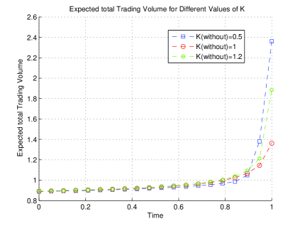
Proposition 4.2 gives the contribution of each group of traders to the total trading volume. From the proof of the proposition 4.1, we know that ωn=0subscript𝜔𝑛0\omega_{n}=0 when K=1𝐾1K=1. Then the term 2αnK2αn+ωn(2αnωn)λn2subscript𝛼𝑛𝐾2subscript𝛼𝑛subscript𝜔𝑛2subscript𝛼𝑛subscript𝜔𝑛subscript𝜆𝑛\frac{2\alpha_{n}K-2\alpha_{n}+\omega_{n}}{(2\alpha_{n}-\omega_{n})\lambda_{n}} in equation (4.45) and (4.44) vanishes when K=1.𝐾1K=1. That is to say both the insider and the market makers trade a larger volume under heterogeneous prior beliefs and thus lead to an increase in total trading volume. Furthermore, σzn2superscriptsubscript𝜎subscript𝑧𝑛2\sigma_{z_{n}}^{2} in equation (4.45) and (4.44) vanishes if there is no public disclosure requirement, i.e., ‘public disclosure’ also makes both the insider and the market makers trade a larger volume and thus lead to an increase in total trading volume.

4.3 Properties of the sequential equilibrium

In order to analyze the properties of the equilibrium, we develop an algorithm that analytically solve the model’s unique equilibrium,333The algorithm here is different form that of Holden and Subrahmanyam (1992). as described in the following proposition.

Proposition 4.3.

Let λn=anΣn1σμsubscript𝜆𝑛subscript𝑎𝑛subscriptΣ𝑛1subscript𝜎𝜇\lambda_{n}=a_{n}\frac{\sqrt{\Sigma_{n-1}}}{\sigma_{\mu}}, αn=bnσμΣn1subscript𝛼𝑛subscript𝑏𝑛subscript𝜎𝜇subscriptΣ𝑛1\alpha_{n}=b_{n}\frac{\sigma_{\mu}}{\sqrt{\Sigma_{n-1}}}, ωn=cnσμΣn1subscript𝜔𝑛subscript𝑐𝑛subscript𝜎𝜇subscriptΣ𝑛1\omega_{n}=c_{n}\frac{\sigma_{\mu}}{\sqrt{\Sigma_{n-1}}}, n=1,2,N.for-all𝑛12𝑁\forall n=1,2,\cdots N. For 0<K<2,0𝐾20<K<2, the solution of the difference equation system in Proposition 4.1 is given by starting the boundary condition bN=0subscript𝑏𝑁0b_{N}=0, cN=0subscript𝑐𝑁0c_{N}=0, aN=K(2K)2subscript𝑎𝑁𝐾2𝐾2a_{N}=\frac{\sqrt{K(2-K)}}{2}, and iterating backward for aN1,,a1subscript𝑎𝑁1subscript𝑎1a_{N-1},\cdots,a_{1}, bN1,,b1subscript𝑏𝑁1subscript𝑏1b_{N-1},\cdots,b_{1} and cN1,,c1subscript𝑐𝑁1subscript𝑐1c_{N-1},\cdots,c_{1} by using the following equation, for n=1,2,N1,𝑛12𝑁1n=1,2\cdots,N-1,

bn1=qn{1+K3qn[(2K)qnzn](2qnzn)2}12,subscript𝑏𝑛1subscript𝑞𝑛superscript1superscript𝐾3subscript𝑞𝑛delimited-[]2𝐾subscript𝑞𝑛subscript𝑧𝑛superscript2subscript𝑞𝑛subscript𝑧𝑛212b_{n-1}=q_{n}\left\{1+\frac{K^{3}q_{n}}{[(2-K)q_{n}-z_{n}](2q_{n}-z_{n})^{2}}\right\}^{\frac{1}{2}}, (4.50)
cn1=zn[1+K3qn[(2K)qnzn][2qnzn)2]12,c_{n-1}=z_{n}\left[1+\frac{K^{3}q_{n}}{[(2-K)q_{n}-z_{n}][2q_{n}-z_{n})^{2}}\right]^{\frac{1}{2}}, (4.51)
an=K2bn(2bncn)2,subscript𝑎𝑛superscript𝐾2subscript𝑏𝑛superscript2subscript𝑏𝑛subscript𝑐𝑛2a_{n}=\frac{K^{2}b_{n}}{(2b_{n}-c_{n})^{2}}, (4.52)

where

qn=subscript𝑞𝑛absent\displaystyle q_{n}= [1K4bn2[(2K)bncn](2bncn)3]K4bn2(2bnK2bn+cn)(2bnKbncn)(2bncn)2K2bn(2bncn)(2bnKbncn)delimited-[]1superscript𝐾4superscriptsubscript𝑏𝑛2delimited-[]2𝐾subscript𝑏𝑛subscript𝑐𝑛superscript2subscript𝑏𝑛subscript𝑐𝑛3superscript𝐾4superscriptsubscript𝑏𝑛22subscript𝑏𝑛𝐾2subscript𝑏𝑛subscript𝑐𝑛2subscript𝑏𝑛𝐾subscript𝑏𝑛subscript𝑐𝑛superscript2subscript𝑏𝑛subscript𝑐𝑛2superscript𝐾2subscript𝑏𝑛2subscript𝑏𝑛subscript𝑐𝑛2subscript𝑏𝑛𝐾subscript𝑏𝑛subscript𝑐𝑛\displaystyle\left[1-\frac{K^{4}b_{n}^{2}}{[(2-K)b_{n}-c_{n}](2b_{n}-c_{n})^{3}}\right]\frac{K^{4}b_{n}^{2}-(2b_{n}K-2b_{n}+c_{n})(2b_{n}-Kb_{n}-c_{n})(2b_{n}-c_{n})^{2}}{K^{2}b_{n}(2b_{n}-c_{n})(2b_{n}-Kb_{n}-c_{n})} (4.53)
+bn[1K3bn[(2K)bncn](2bncn)3]2,subscript𝑏𝑛superscriptdelimited-[]1superscript𝐾3subscript𝑏𝑛delimited-[]2𝐾subscript𝑏𝑛subscript𝑐𝑛superscript2subscript𝑏𝑛subscript𝑐𝑛32\displaystyle+b_{n}\left[1-\frac{K^{3}b_{n}}{[(2-K)b_{n}-c_{n}](2b_{n}-c_{n})^{3}}\right]^{2},
zn=subscript𝑧𝑛absent\displaystyle z_{n}= K2bn(1K)(2bncn)(2bnKbncn)[2KK4bn2[(2K)bncn](2bncn)3](2bnK2bn+cn)(2bncn)K2bnsuperscript𝐾2subscript𝑏𝑛1𝐾2subscript𝑏𝑛subscript𝑐𝑛2subscript𝑏𝑛𝐾subscript𝑏𝑛subscript𝑐𝑛delimited-[]2𝐾superscript𝐾4superscriptsubscript𝑏𝑛2delimited-[]2𝐾subscript𝑏𝑛subscript𝑐𝑛superscript2subscript𝑏𝑛subscript𝑐𝑛32subscript𝑏𝑛𝐾2subscript𝑏𝑛subscript𝑐𝑛2subscript𝑏𝑛subscript𝑐𝑛superscript𝐾2subscript𝑏𝑛\displaystyle\frac{K^{2}b_{n}(1-K)}{(2b_{n}-c_{n})(2b_{n}-Kb_{n}-c_{n})}-\left[2-K-\frac{K^{4}b_{n}^{2}}{[(2-K)b_{n}-c_{n}](2b_{n}-c_{n})^{3}}\right]\frac{(2b_{n}K-2b_{n}+c_{n})(2b_{n}-c_{n})}{K^{2}b_{n}} (4.54)
+cn[1K3bn[(2K)bncn](2bncn)2].subscript𝑐𝑛delimited-[]1superscript𝐾3subscript𝑏𝑛delimited-[]2𝐾subscript𝑏𝑛subscript𝑐𝑛superscript2subscript𝑏𝑛subscript𝑐𝑛2\displaystyle+c_{n}\left[1-\frac{K^{3}b_{n}}{[(2-K)b_{n}-c_{n}](2b_{n}-c_{n})^{2}}\right].

Then starting from the exogenous values Σ0subscriptΣ0\Sigma_{0} and σμ2superscriptsubscript𝜎𝜇2\sigma_{\mu}^{2}, iterate forward for each of the following variables in the order listed

Σn=(1Kan2bnKbncn)Σn1,subscriptΣ𝑛1𝐾subscript𝑎𝑛2subscript𝑏𝑛𝐾subscript𝑏𝑛subscript𝑐𝑛subscriptΣ𝑛1\displaystyle\Sigma_{n}=\left(1-\frac{Ka_{n}}{2b_{n}-Kb_{n}-c_{n}}\right)\Sigma_{n-1}, (4.55)
βn=K4bn2(2bnK2bn+cn)(2bnKbncn)(2bncn)22K2bn(2bnKbncn)2σμΣn1,subscript𝛽𝑛superscript𝐾4superscriptsubscript𝑏𝑛22subscript𝑏𝑛𝐾2subscript𝑏𝑛subscript𝑐𝑛2subscript𝑏𝑛𝐾subscript𝑏𝑛subscript𝑐𝑛superscript2subscript𝑏𝑛subscript𝑐𝑛22superscript𝐾2subscript𝑏𝑛superscript2subscript𝑏𝑛𝐾subscript𝑏𝑛subscript𝑐𝑛2subscript𝜎𝜇subscriptΣ𝑛1\displaystyle\beta_{n}=\frac{K^{4}b_{n}^{2}-(2b_{n}K-2b_{n}+c_{n})(2b_{n}-Kb_{n}-c_{n})(2b_{n}-c_{n})^{2}}{2K^{2}b_{n}(2b_{n}-Kb_{n}-c_{n})^{2}}\frac{\sigma_{\mu}}{\sqrt{\Sigma_{n-1}}}, (4.56)
ηn=K2bncnΣn1σμ,subscript𝜂𝑛𝐾2subscript𝑏𝑛subscript𝑐𝑛subscriptΣ𝑛1subscript𝜎𝜇\displaystyle\eta_{n}=\frac{K}{2b_{n}-c_{n}}\frac{\sqrt{\Sigma_{n-1}}}{\sigma_{\mu}}, (4.57)
θn=2bnK2bn+cnan(2bncn)σμΣn1,subscript𝜃𝑛2subscript𝑏𝑛𝐾2subscript𝑏𝑛subscript𝑐𝑛subscript𝑎𝑛2subscript𝑏𝑛subscript𝑐𝑛subscript𝜎𝜇subscriptΣ𝑛1\displaystyle\theta_{n}=\frac{2b_{n}K-2b_{n}+c_{n}}{a_{n}(2b_{n}-c_{n})}\frac{\sigma_{\mu}}{\sqrt{\Sigma_{n-1}}}, (4.58)
γn=2bnK2bn+cn2bncn,subscript𝛾𝑛2subscript𝑏𝑛𝐾2subscript𝑏𝑛subscript𝑐𝑛2subscript𝑏𝑛subscript𝑐𝑛\displaystyle\gamma_{n}=-\frac{2b_{n}K-2b_{n}+c_{n}}{2b_{n}-c_{n}}, (4.59)
γn=2bnK2bn+cnKbn,superscriptsubscript𝛾𝑛2subscript𝑏𝑛𝐾2subscript𝑏𝑛subscript𝑐𝑛𝐾subscript𝑏𝑛\displaystyle\gamma_{n}^{\prime}=-\frac{2b_{n}K-2b_{n}+c_{n}}{Kb_{n}}, (4.60)
σzn2=Kbn2bnKbncnσμ2K4bn2(2bnKbncn)2(2bncn)2σμ2,superscriptsubscript𝜎subscript𝑧𝑛2𝐾subscript𝑏𝑛2subscript𝑏𝑛𝐾subscript𝑏𝑛subscript𝑐𝑛superscriptsubscript𝜎𝜇2superscript𝐾4superscriptsubscript𝑏𝑛2superscript2subscript𝑏𝑛𝐾subscript𝑏𝑛subscript𝑐𝑛2superscript2subscript𝑏𝑛subscript𝑐𝑛2superscriptsubscript𝜎𝜇2\displaystyle\sigma_{z_{n}}^{2}=\frac{Kb_{n}}{2b_{n}-Kb_{n}-c_{n}}\sigma_{\mu}^{2}-\frac{K^{4}b_{n}^{2}}{(2b_{n}-Kb_{n}-c_{n})^{2}(2b_{n}-c_{n})^{2}}\sigma_{\mu}^{2}, (4.61)

for all n=1,2,,N,𝑛12𝑁n=1,2,\cdots,N, and when n=N𝑛𝑁n=N, the boundary condition is given by Eqs. (4.40)4.40(\ref{eq4.13'}) and (4.41)4.41(\ref{eq4.14'}).

Proof.

See the Appendix. ∎

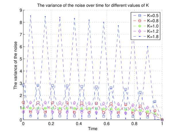
Using formulas in the proposition we generate a series of numerical simulations. We first compare the interesting parameters λnsubscript𝜆𝑛\lambda_{n}, ΣnsubscriptΣ𝑛\Sigma_{n}, E1[Δπ~n]subscript𝐸1delimited-[]Δsubscript~𝜋𝑛E_{1}[\Delta\tilde{\pi}_{n}] and σzn2superscriptsubscript𝜎subscript𝑧𝑛2\sigma_{z_{n}}^{2} in our model with those of Huddart, Hughes and Levine (2001) and Wang (1998). As in Kyle (1985), the parameters ΣnsubscriptΣ𝑛\Sigma_{n} and λnsubscript𝜆𝑛\lambda_{n} are the inverse measures of price efficiency and the market depth, respectively. Δπ~nΔsubscript~𝜋𝑛\Delta\tilde{\pi}_{n} denotes the profits of the n𝑛n-th auction, i.e., Δπ~n=π~n+1π~n.Δsubscript~𝜋𝑛subscript~𝜋𝑛1subscript~𝜋𝑛\Delta\tilde{\pi}_{n}=\tilde{\pi}_{n+1}-\tilde{\pi}_{n}. And σzn2superscriptsubscript𝜎subscript𝑧𝑛2\sigma_{z_{n}}^{2} denotes the variance of the noise that the insider put when he plays mixed strategy in the n𝑛n-th period.


Refer to caption
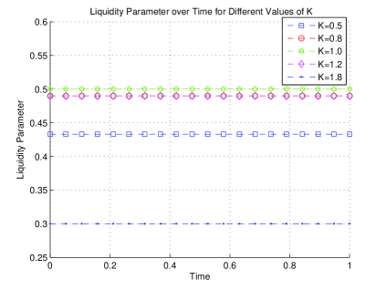
(a) Liquidity parameters, λnsubscript𝜆𝑛\lambda_{n}, when the insider must disclosure each trade ex-post, are plotted over time for different values of K𝐾K, K=0.5𝐾0.5K=0.5, K=0.8𝐾0.8K=0.8, K=1.0𝐾1.0K=1.0, K=1.2𝐾1.2K=1.2, K=1.8𝐾1.8K=1.8.
Refer to caption
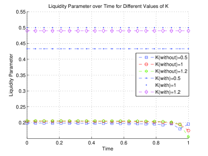
(b) The liquidity parameter at each auction is plotted for different value of K𝐾K, K=0.5𝐾0.5K=0.5, K=1.0𝐾1.0K=1.0, K=1.2𝐾1.2K=1.2. K(without)𝐾𝑤𝑖𝑡𝑜𝑢𝑡K(without) in the figure means the K𝐾K in the model that no public disclosure of insider trade is required, and K(with)𝐾𝑤𝑖𝑡K(with) means the K𝐾K in the model that the insider must disclose each trade ex post.
Figure 1: Numeric solutions of the liquidity parameters λnsubscript𝜆𝑛\lambda_{n} with one unit of initial variance of information.


Refer to caption
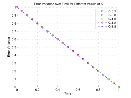
(a) The Error variances of price, ΣnsubscriptΣ𝑛\Sigma_{n}, when the insider must disclosure each trade ex post, are plotted over time for different values of K𝐾K, K=0.5𝐾0.5K=0.5, K=0.8𝐾0.8K=0.8, K=1.0𝐾1.0K=1.0, K=1.2𝐾1.2K=1.2, K=1.8𝐾1.8K=1.8.
Refer to caption
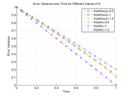
(b) The error variance of price at each auction is plotted for different value of K𝐾K, K=0.5𝐾0.5K=0.5, K=1𝐾1K=1, K=1.2𝐾1.2K=1.2. K(without) in the figure means the K𝐾K in the model that no public disclosure of insider trade is required, and K(with) means the K𝐾K in the model that the insider must disclose each trade ex-post.
Figure 2: Numeric solutions of the error variance of price, ΣnsubscriptΣ𝑛\Sigma_{n}, with one unit of initial variance of information.

Figure 111 and Figure 222 plot the dynamic behavior of the liquidity parameter λnsubscript𝜆𝑛\lambda_{n} and the error variance of price ΣnsubscriptΣ𝑛\Sigma_{n}, respectively, by holding constants N=20𝑁20N=20, Σ0=1subscriptΣ01\Sigma_{0}=1 and σμ2=1superscriptsubscript𝜎𝜇21\sigma_{\mu}^{2}=1 fixed and varying the belief parameter K=0.5,0.8,1.0,1.2𝐾0.50.81.01.2K=0.5,0.8,1.0,1.2, or 1.8.1.81.8. Among them, the subfigures 1(a)1𝑎1(a) and 2(a)2𝑎2(a) plot the parameters λnsubscript𝜆𝑛\lambda_{n} and ΣnsubscriptΣ𝑛\Sigma_{n} in our model respectively for different values K𝐾K, while the subfigures 1(b)1𝑏1(b) and 2(b)2𝑏2(b) contrast the parameters λnsubscript𝜆𝑛\lambda_{n} and ΣnsubscriptΣ𝑛\Sigma_{n}, respectively, (i) when the insider must disclose each trade ex-post and (ii) when no such disclosures are made.

Figure 1(a)1𝑎1(a) shows the trajectory of the market maker’s price adjustment λnsubscript𝜆𝑛\lambda_{n} in our model for varying belief parameters. It indicates that the liquidity parameter λnsubscript𝜆𝑛\lambda_{n} is constant for any values of K𝐾K. This result is consistent with that of Huddart, Hughes and Levine (2001). It also indicates that the market depth, measured by 1λn1subscript𝜆𝑛\frac{1}{\lambda_{n}}, is positively related to the degree of heterogeneity, measured by |K1|𝐾1|K-1|. Figure 1(b)1𝑏1(b) indicates that “public disclosure” not only leads to constant market depth for any values of K𝐾K, but also makes the adverse selection (measured by λnsubscript𝜆𝑛\lambda_{n}) higher than the case of without public disclosure requirements. This is because under the requirements of disclosure the information content of the order flow is high.
The pattern of λnsubscript𝜆𝑛\lambda_{n} is consistent with the released speed of the information of the insider, measured by ΣnsubscriptΣ𝑛\Sigma_{n}, which is plotted in Figure 222. Figure 2(a)2𝑎2(a) indicates that when the insider must disclose, the value of ΣnsubscriptΣ𝑛\Sigma_{n} following each disclosure declines linearly over time independent of periods and the values of K𝐾K. However, Figure 2(b)2𝑏2(b) indicates that less information asymmetry is present in the market with more aggressive informed trading, measured by the parameter K𝐾K, without public disclosure requirements.
  

Refer to caption
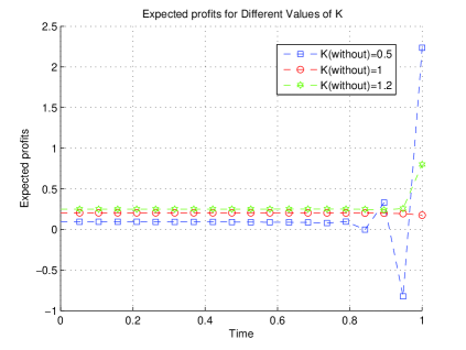
(a) Expected profit, E(Δπ~n)𝐸Δsubscript~𝜋𝑛E(\Delta\tilde{\pi}_{n}), when the insider must disclosure each trade ex-post, are plotted over time for different values of K𝐾K, K=0.5𝐾0.5K=0.5, K=0.8𝐾0.8K=0.8, K=1.0𝐾1.0K=1.0, K=1.2𝐾1.2K=1.2, K=1.8𝐾1.8K=1.8.
Refer to caption
(b) Expected profit E(Δπ~n)𝐸Δsubscript~𝜋𝑛E(\Delta\tilde{\pi}_{n}) at each auction is plotted for different value of K𝐾K, K=0.5𝐾0.5K=0.5, K=1𝐾1K=1, K=1.2𝐾1.2K=1.2. K(without) in the figure means the K𝐾K in the model that no public disclosure of insider trade is required.
Figure 3: Numeric solutions of the expected profit E(Δπ~n)𝐸Δsubscript~𝜋𝑛E(\Delta\tilde{\pi}_{n}) with one unit of initial variance of information.
Refer to caption
Figure 4: The variances of the noise that the insider play, σzn2superscriptsubscript𝜎subscript𝑧𝑛2\sigma_{z_{n}}^{2}, are plotted over time for different values of K𝐾K, K=0.5𝐾0.5K=0.5, K=1.0𝐾1.0K=1.0, K=1.2𝐾1.2K=1.2, K=1.5𝐾1.5K=1.5, K=1.8𝐾1.8K=1.8.

In order to see the differences between the heterogeneous priors case to the common priors case, and the cases with and without public disclosure requirements clearly, we plot the dynamic behavior of E1[Δπ~n]subscript𝐸1delimited-[]Δsubscript~𝜋𝑛E_{1}[\Delta\tilde{\pi}_{n}] of the two cases, respectively, in Figure 333. Figure 3(a)3𝑎3(a) shows that the expected profits of the rational insider are constant over trading rounds. This is the result of Huddart, Hughes and Levine (2001). An interesting result can be get from Figure 3(a)3𝑎3(a) is that the insider’s profits fluctuate greatly if the insider is underconfident or overconfident. Specifically, the sign of the expected profit is alternating to ensure the last sign of the last period is not negative. Moreover, the dynamic pattern in Figure 3(a)3𝑎3(a) indicates that the fluctuation of the expected profits is positively related to the degree of heterogeneity, measured by |K1|𝐾1|K-1|. Even though “disclosure requirement” makes the profits of some trading rounds are negative, the insider trading can also profit from the whole trading process. While without the public disclosure of insider trades, the expected profit at each period is almost constant in all early auctions and becomes significant only in the last few ones.

Figure 444 indicates that the fluctuation of the noise’s variance is bigger at the beginning few periods and becomes smaller gradually if the the insider is irrational. The degree of noise variance’s fluctuation is positively related to the degree of heterogeneity, measured by |K1|𝐾1|K-1|. Figure 444 also indicates that more overconfident insider puts an smaller noise at the first period and then put a bigger one, while the more under confident insider does the opposite.
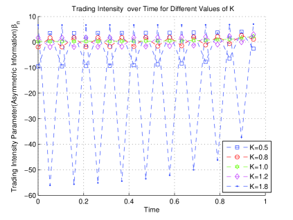
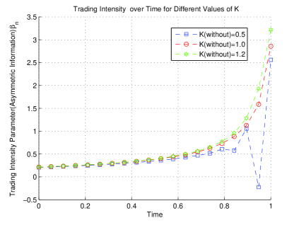
  

Refer to caption
(a) The intensities of trading on private information, measured by βnsubscript𝛽𝑛\beta_{n}, are plotted over time for different values of K𝐾K, when the insider must disclosure each trade ex-post.
Refer to caption
(b) The intensity of trading on private information at each auction is plotted for different value of K𝐾K, K=0.5𝐾0.5K=0.5, K=1𝐾1K=1, K=1.2𝐾1.2K=1.2. K(without)𝐾𝑤𝑖𝑡𝑜𝑢𝑡K(without) in the figure means the K𝐾K in the model that no public disclosure of insider trade is required.
Figure 5: The intensity of trading on information, βnsubscript𝛽𝑛\beta_{n}, over time for different values of K𝐾K are plotted.


Refer to caption
(a) The intensities of trading on heterogeneous prior beliefs, measured by θnsubscript𝜃𝑛\theta_{n}, are plotted over time for different values of K𝐾K, when the insider must disclosure each trade ex-post. The number of auctions is fixed at N=20𝑁20N=20 and the error variance at each auction is plotted for different value of K𝐾K, K=0.5𝐾0.5K=0.5, K=0.8𝐾0.8K=0.8, K=1.0𝐾1.0K=1.0, K=1.2𝐾1.2K=1.2, K=1.8𝐾1.8K=1.8.
Refer to caption
(b) The intensities of trading on heterogeneous prior beliefs at each auction are plotted for different value of K𝐾K, K=0.5𝐾0.5K=0.5, K=1𝐾1K=1, K=1.2𝐾1.2K=1.2. K(without) in the figure means the K𝐾K in the model that no public disclosure of insider trade is required.
Figure 6: The intensity of trading on heterogeneous prior beliefs, θnsubscript𝜃𝑛\theta_{n}, over time for different values of K𝐾K are plotted.


Refer to caption
(a) The heterogeneity parameters, γnsubscript𝛾𝑛\gamma_{n},are plotted over time for different values of K𝐾K, when the insider must disclosure each trade ex post. The number of auctions is fixed at N=20𝑁20N=20 and the error variance at each auction is plotted for different value of K𝐾K, K=0.5𝐾0.5K=0.5, K=0.8𝐾0.8K=0.8, K=1.0𝐾1.0K=1.0, K=1.2𝐾1.2K=1.2, K=1.8𝐾1.8K=1.8.
Refer to caption
(b) The heterogeneity parameter, γnsubscript𝛾𝑛\gamma_{n}, at each auction is plotted for different value of K𝐾K, K=0.5𝐾0.5K=0.5, K=1𝐾1K=1, K=1.2𝐾1.2K=1.2. K(without)𝐾𝑤𝑖𝑡𝑜𝑢𝑡K(without) in the figure means the K𝐾K in the model that no public disclosure of insider trade is required.
Figure 7: The intensity of trading on heterogeneous prior beliefs, θnsubscript𝜃𝑛\theta_{n}, over time for different values of K𝐾K are plotted.
Refer to caption
Figure 8: The heterogeneous parameters, γnsuperscriptsubscript𝛾𝑛\gamma_{n}^{\prime}, over time for different values of K𝐾K are plotted, when the insider must disclosure each trade ex post. The number of auctions is fixed at N=20𝑁20N=20 and the liquidity parameter at each auction is plotted for different value of K𝐾K, K=0.5𝐾0.5K=0.5, K=1.0𝐾1.0K=1.0, K=1.2𝐾1.2K=1.2, K=1.5𝐾1.5K=1.5, K=1.8𝐾1.8K=1.8.


Refer to caption
(a) The expected total trading volume, Voln𝑉𝑜subscript𝑙𝑛Vol_{n}, over time for different values of K𝐾K are plotted, when the insider must disclosure each trade ex post. The number of auctions is fixed at N=20𝑁20N=20 and the liquidity parameter at each auction is plotted for different value of K𝐾K, K=0.5𝐾0.5K=0.5, K=0.8𝐾0.8K=0.8, K=1.0𝐾1.0K=1.0, K=1.2𝐾1.2K=1.2, K=1.8𝐾1.8K=1.8.
Refer to caption
(b) The expected total trading volume at each auction is plotted for different value of K𝐾K, K=0.5𝐾0.5K=0.5, K=1.0𝐾1.0K=1.0, K=1.2𝐾1.2K=1.2. K(without)𝐾𝑤𝑖𝑡𝑜𝑢𝑡K(without) in the figure means the K𝐾K in the model that no public disclosure of insider trade is required.
Figure 9: Numeric solutions of the expected total trading volume Voln𝑉𝑜subscript𝑙𝑛Vol_{n} with one unit of initial variance of information.

Next, we compare parameters βnsubscript𝛽𝑛\beta_{n}, θnsubscript𝜃𝑛\theta_{n}, γnsubscript𝛾𝑛\gamma_{n} γnsuperscriptsubscript𝛾𝑛\gamma_{n}^{\prime} and Voln𝑉𝑜subscript𝑙𝑛Vol_{n} between the case of with and without disclosure of insider trades for varying numbers of trading rounds, by holding constants N=20𝑁20N=20, Σ0=1subscriptΣ01\Sigma_{0}=1 and σμ2=1superscriptsubscript𝜎𝜇21\sigma_{\mu}^{2}=1 fixed and varying the belief parameter K=0.5𝐾0.5K=0.5, 0.80.80.8, 1.01.01.0, 1.21.21.2, or 1.8.1.81.8. As in Wang (1998), βnsubscript𝛽𝑛{\beta_{n}} measures the trading intensity on the asymmetric information, θnsubscript𝜃𝑛\theta_{n} measures the trading intensity on heterogeneous beliefs, γnsubscript𝛾𝑛\gamma_{n} and γnsuperscriptsubscript𝛾𝑛\gamma_{n}^{\prime} are heterogeneity parameters, and Voln𝑉𝑜subscript𝑙𝑛Vol_{n} measures the total expected trading volume.

Figure 5(a)5𝑎5(a) indicates that under the disclosure requirement the irrational informed trader’s intensity of trading on asymmetric information, measured by βnsubscript𝛽𝑛{\beta_{n}}, fluctuates greatly during all early auctions and becomes subdued gradually in the last few rounds of trades. The fluctuation is also positively related to the degree of the heterogeneity. This result is intuitive since the more heterogeneous informed trader is the more he will be influenced by the “trade disclosure” and more aggressively he will trade. Figure 5(a)5𝑎5(a) also indicates if the insider is overconfident the intensity of trading is positive at the first period and negative at the second period, and the sigh changes alternatively, while the underconfident insider does the opposite. This result is very differently from the case of no disclosure requirement, which is given in Figure 5(b)5𝑏5(b).
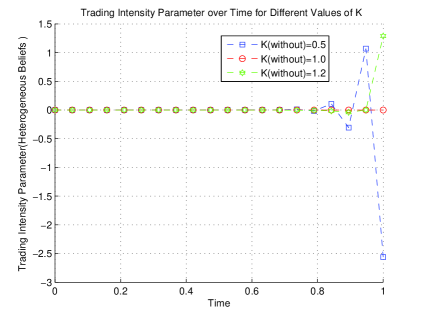
Figure 6(a)6𝑎6(a) shows that the irrational informed trader’s intensity of trading on heterogeneous prior beliefs, measured by θnsubscript𝜃𝑛{\theta_{n}}, also fluctuates greatly during all early auctions and the fluctuation is also positively related to the degree of heterogeneity, but the direction of fluctuation is opposite to that of βnsubscript𝛽𝑛\beta_{n}. That is to say if the irrational insider puts a positive weight on asymmetric information this period, then he puts a negative weight on heterogeneous prior beliefs, and the case is inverse in the next period. While Figure 6(b)6𝑏6(b) shows that the informed trader trades on differences in beliefs only in the last few auctions since the intensity of trading on heterogeneous prior beliefs is negligible in all early auctions, which is the result of Wang (1998). Comparing the Figure 5(a)5𝑎5(a) with Figure 5(b)5𝑏5(b), and 6(a)6𝑎6(a) with Figure 6(a)6𝑎6(a) we know that ‘trade disclosure’ has a big influence on the insider’s strategy, whenever the insider is underconfident or overconfident.

Figure 777 and Figure 888 plot the heterogeneity parameters γnsubscript𝛾𝑛\gamma_{n} and γnsuperscriptsubscript𝛾𝑛\gamma_{n}^{\prime}, respectively. They indicate that γnsubscript𝛾𝑛\gamma_{n} and γnsuperscriptsubscript𝛾𝑛\gamma_{n}^{\prime} all also fluctuate according to the degree of heterogeneity. This pattern is consistent with the informed trader’s strategies. Market makers can correctly predict that “heterogeneous prior beliefs” and “trade disclosure” have big impacts on the trader’s strategies at each auction, market makers choose a non-zero γnsubscript𝛾𝑛\gamma_{n} to account for the adverse selection problem properly, and adjust γnsubscript𝛾𝑛\gamma_{n} to γnsuperscriptsubscript𝛾𝑛\gamma_{n}^{\prime} correctly after observing the insider’s trading. This intuition is further confirmed by the fact that the patterns in Figure 7(a)7𝑎7(a) and Figure 888 are exactly the opposites of the pattern in Figure 6(a)6𝑎6(a).

Figure 9(a)9𝑎9(a) indicates that the total expected trading volume Voln𝑉𝑜subscript𝑙𝑛Vol_{n}, is positively related to the degree of heterogeneity, measured by |K1|.𝐾1|K-1|. The fluctuation is greatly during all early auctions and becomes subdued gradually in the last few rounds of trades, this pattern is consistent with that of the trading strategy of the insider. Comparing Figure 9(a)9𝑎9(a) with Figure 9(b)9𝑏9(b), we how that under the requirement of public disclosure, the expected trading volume is dramatically big. This result vividly confirms Proposition 4.2 which shows that not only “heterogeneous prior beliefs” but also “public disclosure” lead to a larger volume.

5 Conclusions

In this paper, we have characterized the dynamically optimal trading strategies of an irrational insider under ex-post disclosure requirement, and addressed the impacts on the financial markets.

In contrast to the case of an irrational insider who restricts his intensity of trading on private information, during all early auctions and becomes aggressive only in the last few rounds of trades in a setting under no disclosure requirement, we show that the irrational insider under disclosure requirement employs a mixed strategy and trades more aggressive on private information from the beginning to the end. In particular, under disclosure requirements, insider puts the weights on asymmetric information and heterogeneous prior beliefs are opposite in sign, and the sighs change alternatively in the next period. Since on one hand the irrational insider is overconfident or underconfident about his signal and on the other hand he wants to dissimulates his information, he trades more aggressively than he rational does. The market makers, realizing the heterogeneity and that a part of total order flow is due to aggressive behavior, increases market depth. Also, under disclosure requirement, the market depth is positive related to the degree of the heterogeneity.

Our model indicates that despite the irrational insider dissembles his information by adding a random component to his trades, the information is reflected more rapidly in price with the disclosure of insider trades than without. An interesting find is that “public disclosure” makes the revelation speed of the information are the same, whenever the insider is overconfident or underconfident. In equilibrium, we also show that while “public disclosure” may lead to negative profits at some trading rounds, insider trading remains profitable from the whole trading time. The irrational insider trades to make sure his profit at the last period is positive. Furthermore, the heterogeneity beliefs and public disclosure all lead to larger trading volume. The co-existence of the heterogeneity beliefs and public disclosure makes the trading volume fluctuate greatly, and the fluctuation is positive related to the degree of the insider’s heterogeneity. This result can explain the trading fluctuation in the real finance in some sense.

Appendix

Proof of Proposition 3.1: Let the N𝑁N in Theorem 111 of Wang (1998) equal 222 and ΔtnΔsubscript𝑡𝑛\Delta t_{n} equal 111 (n=1,2)𝑛12(n=1,2), we have the following relationships:

α2=ω2=ϕ2=δ2=0,β2=12λ2,θ2=γ2λ2,formulae-sequencesubscript𝛼2subscript𝜔2subscriptitalic-ϕ2subscript𝛿20formulae-sequencesubscript𝛽212subscript𝜆2subscript𝜃2subscript𝛾2subscript𝜆2\alpha_{2}=\omega_{2}=\phi_{2}=\delta_{2}=0,~{}~{}\beta_{2}=\frac{1}{2\lambda_{2}},~{}~{}\theta_{2}=-\frac{\gamma_{2}}{\lambda_{2}},
λ2=[(1+γ2)β2+θ2]Σ2σμ2,γ2=1K,Σ2=(1+γ2)(1λ2β2)Σ1,formulae-sequencesubscript𝜆2delimited-[]1subscript𝛾2subscript𝛽2subscript𝜃2subscriptΣ2superscriptsubscript𝜎𝜇2formulae-sequencesubscript𝛾21𝐾subscriptΣ21subscript𝛾21subscript𝜆2subscript𝛽2subscriptΣ1\lambda_{2}=\frac{[(1+\gamma_{2})\beta_{2}+\theta_{2}]\Sigma_{2}}{\sigma_{\mu}^{2}},~{}~{}\gamma_{2}=1-K,~{}~{}\Sigma_{2}=(1+\gamma_{2})(1-\lambda_{2}\beta_{2})\Sigma_{1},
α1=(1+γ2)24λ2,ω1=(2K)γ2λ2,ϕ1=γ2λ2,δ1=0,formulae-sequencesubscript𝛼1superscript1subscript𝛾224subscript𝜆2formulae-sequencesubscript𝜔12𝐾subscript𝛾2subscript𝜆2formulae-sequencesubscriptitalic-ϕ1subscript𝛾2subscript𝜆2subscript𝛿10\alpha_{1}=\frac{(1+\gamma_{2})^{2}}{4\lambda_{2}},~{}~{}~{}\omega_{1}=\frac{(2-K)\gamma_{2}}{\lambda_{2}},~{}~{}~{}\phi_{1}=-\frac{\gamma_{2}}{\lambda_{2}},~{}~{}~{}\delta_{1}=0,
β1=12α1λ12λ1(1α1λ1),θ1=γ1λ1,λ1=[(1+γ1)β1+θ1]Σ1σμ2,formulae-sequencesubscript𝛽112subscript𝛼1subscript𝜆12subscript𝜆11subscript𝛼1subscript𝜆1formulae-sequencesubscript𝜃1subscript𝛾1subscript𝜆1subscript𝜆1delimited-[]1subscript𝛾1subscript𝛽1subscript𝜃1subscriptΣ1superscriptsubscript𝜎𝜇2\beta_{1}=\frac{1-2\alpha_{1}\lambda_{1}}{2\lambda_{1}(1-\alpha_{1}\lambda_{1})},~{}~{}~{}\theta_{1}=-\frac{\gamma_{1}}{\lambda_{1}},~{}~{}\lambda_{1}=\frac{[(1+\gamma_{1})\beta_{1}+\theta_{1}]\Sigma_{1}}{\sigma_{\mu}^{2}},
γ1=1Kω1λ1,Σ1=(1+γ1)(1λ1β1)Σ0,formulae-sequencesubscript𝛾11𝐾subscript𝜔1subscript𝜆1subscriptΣ11subscript𝛾11subscript𝜆1subscript𝛽1subscriptΣ0\gamma_{1}=1-K-\omega_{1}\lambda_{1},~{}~{}~{}\Sigma_{1}=(1+\gamma_{1})(1-\lambda_{1}\beta_{1})\Sigma_{0},
α0=(1+γ1)24λ1(1α1λ1),ω0=ω1+(2K)γ1λ1,ϕ0=ϕ1γ1λ1,δ0=α1λ12σμ2.formulae-sequencesubscript𝛼0superscript1subscript𝛾124subscript𝜆11subscript𝛼1subscript𝜆1formulae-sequencesubscript𝜔0subscript𝜔12𝐾subscript𝛾1subscript𝜆1formulae-sequencesubscriptitalic-ϕ0subscriptitalic-ϕ1subscript𝛾1subscript𝜆1subscript𝛿0subscript𝛼1superscriptsubscript𝜆12superscriptsubscript𝜎𝜇2\alpha_{0}=\frac{(1+\gamma_{1})^{2}}{4\lambda_{1}(1-\alpha_{1}\lambda_{1})},~{}~{}\omega_{0}=\omega_{1}+\frac{(2-K)\gamma_{1}}{\lambda_{1}},~{}~{}~{}~{}\phi_{0}=\phi_{1}-\frac{\gamma_{1}}{\lambda_{1}},~{}~{}~{}\delta_{0}=\alpha_{1}\lambda_{1}^{2}\sigma_{\mu}^{2}.

By γ2=1Ksubscript𝛾21𝐾\gamma_{2}=1-K we can get

β2=12λ2,θ2=K1λ2,λ22=KΣ22σμ2,Σ2=(1K2)Σ1,formulae-sequencesubscript𝛽212subscript𝜆2formulae-sequencesubscript𝜃2𝐾1subscript𝜆2formulae-sequencesuperscriptsubscript𝜆22𝐾subscriptΣ22superscriptsubscript𝜎𝜇2subscriptΣ21𝐾2subscriptΣ1\beta_{2}=\frac{1}{2\lambda_{2}},~{}~{}~{}\theta_{2}=\frac{K-1}{\lambda_{2}},~{}~{}~{}\lambda_{2}^{2}=\frac{K\Sigma_{2}}{2\sigma_{\mu}^{2}},~{}~{}\Sigma_{2}=(1-\frac{K}{2})\Sigma_{1},
α1=(2K)24λ2,ω1=(2K)(1K)λ2,ϕ1=K1λ2.formulae-sequencesubscript𝛼1superscript2𝐾24subscript𝜆2formulae-sequencesubscript𝜔12𝐾1𝐾subscript𝜆2subscriptitalic-ϕ1𝐾1subscript𝜆2\alpha_{1}=\frac{(2-K)^{2}}{4\lambda_{2}},~{}~{}\omega_{1}=\frac{(2-K)(1-K)}{\lambda_{2}},~{}~{}~{}\phi_{1}=\frac{K-1}{\lambda_{2}}.

From the second order condition, λ2>0subscript𝜆20\lambda_{2}>0, we can get λ2=KΣ22σμ2subscript𝜆2𝐾subscriptΣ22superscriptsubscript𝜎𝜇2\lambda_{2}=\sqrt{\frac{K\Sigma_{2}}{2\sigma_{\mu}^{2}}}. From the above we know that if we get Σ2subscriptΣ2\Sigma_{2}, then we can get λ2subscript𝜆2\lambda_{2}, and all the coefficients of the second period is known. But in order to get Σ2subscriptΣ2\Sigma_{2}, we first solve Σ1subscriptΣ1\Sigma_{1}. Combing the expression of α1subscript𝛼1\alpha_{1} and β1subscript𝛽1\beta_{1}, we get

β1=[2m(2K)2]λ1[4m(2K)2].subscript𝛽1delimited-[]2𝑚superscript2𝐾2subscript𝜆1delimited-[]4𝑚superscript2𝐾2\beta_{1}=\frac{[2-m(2-K)^{2}]}{\lambda_{1}[4-m(2-K)^{2}]}. (5.62)

The expression of γ1subscript𝛾1\gamma_{1} and ω1subscript𝜔1\omega_{1} imply

γ1=(1K)[1m(2K)],θ1=γ1λ1,Σ1=2(2K)[1m(1K)]Σ04m(2K)2.formulae-sequencesubscript𝛾11𝐾delimited-[]1𝑚2𝐾formulae-sequencesubscript𝜃1subscript𝛾1subscript𝜆1subscriptΣ122𝐾delimited-[]1𝑚1𝐾subscriptΣ04𝑚superscript2𝐾2\gamma_{1}=(1-K)[1-m(2-K)],~{}~{}\theta_{1}=-\frac{\gamma_{1}}{\lambda_{1}},~{}~{}\Sigma_{1}=\frac{2(2-K)[1-m(1-K)]\Sigma_{0}}{4-m(2-K)^{2}}. (5.63)

where mλ1λ2approaches-limit𝑚subscript𝜆1subscript𝜆2m\doteq\frac{\lambda_{1}}{\lambda_{2}}.

Substitute the expression of β1,γ1,θ1subscript𝛽1subscript𝛾1subscript𝜃1\beta_{1},\gamma_{1},\theta_{1} and Σ1subscriptΣ1\Sigma_{1} into λ1=[(1+γ1)β1+θ1]Σ1σμ2subscript𝜆1delimited-[]1subscript𝛾1subscript𝛽1subscript𝜃1subscriptΣ1superscriptsubscript𝜎𝜇2\lambda_{1}=\frac{[(1+\gamma_{1})\beta_{1}+\theta_{1}]\Sigma_{1}}{\sigma_{\mu}^{2}}, we obtain

λ12=1σμ22K(2K)[2m(2K)][1m(1K)]Σ0[4m(2K)2]2.superscriptsubscript𝜆121superscriptsubscript𝜎𝜇22𝐾2𝐾delimited-[]2𝑚2𝐾delimited-[]1𝑚1𝐾subscriptΣ0superscriptdelimited-[]4𝑚superscript2𝐾22\lambda_{1}^{2}=\frac{1}{\sigma_{\mu}^{2}}\frac{2K(2-K)[2-m(2-K)][1-m(1-K)]\Sigma_{0}}{[4-m(2-K)^{2}]^{2}}.

When 4m(2K)2>04𝑚superscript2𝐾204-m(2-K)^{2}>0, [2m(2K)][1m(1K)]>0delimited-[]2𝑚2𝐾delimited-[]1𝑚1𝐾0[2-m(2-K)][1-m(1-K)]>0, i.e. 0<m<22K0𝑚22𝐾0<m<\frac{2}{2-K}

λ1=1σμ2K(2K)[2m(2K)][1m(1K)]Σ04m(2K)2.subscript𝜆11subscript𝜎𝜇2𝐾2𝐾delimited-[]2𝑚2𝐾delimited-[]1𝑚1𝐾subscriptΣ04𝑚superscript2𝐾2\lambda_{1}=\frac{1}{\sigma_{\mu}}\frac{\sqrt{2K(2-K)[2-m(2-K)][1-m(1-K)]\Sigma_{0}}}{4-m(2-K)^{2}}.

By the expression of Σ1subscriptΣ1\Sigma_{1}, we get

Σ2=2K2Σ1=(2K)2[1m(1K)]4m(2K)2Σ0,subscriptΣ22𝐾2subscriptΣ1superscript2𝐾2delimited-[]1𝑚1𝐾4𝑚superscript2𝐾2subscriptΣ0\Sigma_{2}=\frac{2-K}{2}\Sigma_{1}=\frac{(2-K)^{2}[1-m(1-K)]}{4-m(2-K)^{2}}\Sigma_{0},
λ2=KΣ22σμ2=12σμ2K(2K)2[1m(1K)]Σ04m(2K)2.subscript𝜆2𝐾subscriptΣ22superscriptsubscript𝜎𝜇212subscript𝜎𝜇2𝐾superscript2𝐾2delimited-[]1𝑚1𝐾subscriptΣ04𝑚superscript2𝐾2\lambda_{2}=\sqrt{\frac{K\Sigma_{2}}{2\sigma_{\mu}^{2}}}=\frac{1}{2\sigma_{\mu}}\sqrt{\frac{2K(2-K)^{2}[1-m(1-K)]\Sigma_{0}}{4-m(2-K)^{2}}}.

Since mλ1λ2approaches-limit𝑚subscript𝜆1subscript𝜆2m\doteq\frac{\lambda_{1}}{\lambda_{2}} , we have

m=22m(2K)(2K)[4m(2K)2]𝑚22𝑚2𝐾2𝐾delimited-[]4𝑚superscript2𝐾2m=2\sqrt{\frac{2-m(2-K)}{(2-K)[4-m(2-K)^{2}]}}

i.e.

(2K)3m34(2K)m24(2K)m+8=0,superscript2𝐾3superscript𝑚342𝐾superscript𝑚242𝐾𝑚80(2-K)^{3}m^{3}-4(2-K)m^{2}-4(2-K)m+8=0,

and m𝑚m satisfy 0<m<22K0𝑚22𝐾0<m<\frac{2}{2-K}, m<4(2K)2.𝑚4superscript2𝐾2m<\frac{4}{(2-K)^{2}}. From 0<K<20𝐾20<K<2 we get 0<m<22K0𝑚22𝐾0<m<\frac{2}{2-K}. In order to explain the root that satisfy the condition is unique, let f(m)=(2K)3m34(2K)m24(2K)m+8𝑓𝑚superscript2𝐾3superscript𝑚342𝐾superscript𝑚242𝐾𝑚8f(m)=(2-K)^{3}m^{3}-4(2-K)m^{2}-4(2-K)m+8. It is easy to know f(0)=8>0𝑓080f(0)=8>0, f(22K)=8K2K<0𝑓22𝐾8𝐾2𝐾0f(\frac{2}{2-K})=-\frac{8K}{2-K}<0, so the needed root is unique. Q.E.D.

Proof of Proposition 3.2: In order to get the proposition, we only need to compute E1(π~1)subscript𝐸1subscript~𝜋1E_{1}(\tilde{\pi}_{1}) and E1(π~2).subscript𝐸1subscript~𝜋2E_{1}(\tilde{\pi}_{2}).

Using Eq. (3.3), we can get

E1(π~2)=subscript𝐸1subscript~𝜋2absent\displaystyle E_{1}(\tilde{\pi}_{2})= E1{EK[π~2(p~1,s~)|x~1,p1~,s~]}=E1{14λ2[Ks~(1+γ2)p~1]2}subscript𝐸1subscript𝐸𝐾delimited-[]conditionalsubscript~𝜋2superscriptsubscript~𝑝1~𝑠subscript~𝑥1~superscriptsubscript𝑝1~𝑠subscript𝐸114subscript𝜆2superscriptdelimited-[]𝐾~𝑠1subscript𝛾2superscriptsubscript~𝑝12\displaystyle E_{1}\{E_{K}[\tilde{\pi}_{2}(\tilde{p}_{1}^{*},\tilde{s})|\tilde{x}_{1},\tilde{p_{1}^{*}},\tilde{s}]\}=E_{1}\left\{\frac{1}{4\lambda_{2}}[K\tilde{s}-(1+\gamma_{2})\tilde{p}_{1}^{*}]^{2}\right\} (5.64)
=\displaystyle= 14λ2{K2Σ1+(2K2)2E1[(1+γ1)p0+η1x~1]2}14subscript𝜆2superscript𝐾2subscriptΣ1superscript2𝐾22subscript𝐸1superscriptdelimited-[]1superscriptsubscript𝛾1subscript𝑝0subscript𝜂1subscript~𝑥12\displaystyle\frac{1}{4\lambda_{2}}\left\{K^{2}\Sigma_{1}+(2K-2)^{2}E_{1}[(1+\gamma_{1}^{\prime})p_{0}+\eta_{1}\tilde{x}_{1}]^{2}\right\}
=\displaystyle= K2Σ14λ2+(2K2)24λ2[η12(β1+θ1)2Σ0+(η1θ1+K2K)2p02+η12σz12].superscript𝐾2subscriptΣ14subscript𝜆2superscript2𝐾224subscript𝜆2delimited-[]superscriptsubscript𝜂12superscriptsubscript𝛽1subscript𝜃12subscriptΣ0superscriptsubscript𝜂1subscript𝜃1𝐾2𝐾2superscriptsubscript𝑝02superscriptsubscript𝜂12superscriptsubscript𝜎subscript𝑧12\displaystyle\frac{K^{2}\Sigma_{1}}{4\lambda_{2}}+\frac{(2K-2)^{2}}{4\lambda_{2}}[\eta_{1}^{2}(\beta_{1}+\theta_{1})^{2}\Sigma_{0}+(\eta_{1}\theta_{1}+\frac{K}{2-K})^{2}p_{0}^{2}+\eta_{1}^{2}\sigma_{z_{1}}^{2}].

Substitute the expression of η1,β1,θ1subscript𝜂1subscript𝛽1subscript𝜃1\eta_{1},\beta_{1},\theta_{1} and σz12superscriptsubscript𝜎subscript𝑧12\sigma_{z_{1}}^{2} into the above equation, yields

E1(π~2)=KKΣ0σμ22(2K)+(2K2)2σμ2K(2K)Σ0×\displaystyle E_{1}(\tilde{\pi}_{2})=\frac{K\sqrt{K\Sigma_{0}}\sigma_{\mu}}{2\sqrt{2(2-K)}}+\frac{(2K-2)^{2}\sigma_{\mu}}{\sqrt{2K(2-K)\Sigma_{0}}}\times (5.65)
{KΣ02(2K)σμ2σμ2Σ02K2KΣ0+[KΣ0σμ2(2K)22(1K)σμK(2K)Σ0+K2K]2p02+KΣ02(2K)σμ22K2Kσμ2}𝐾subscriptΣ022𝐾superscriptsubscript𝜎𝜇2superscriptsubscript𝜎𝜇2subscriptΣ02𝐾2𝐾subscriptΣ0superscriptdelimited-[]𝐾subscriptΣ0subscript𝜎𝜇22𝐾221𝐾subscript𝜎𝜇𝐾2𝐾subscriptΣ0𝐾2𝐾2superscriptsubscript𝑝02𝐾subscriptΣ022𝐾superscriptsubscript𝜎𝜇22𝐾2𝐾superscriptsubscript𝜎𝜇2\displaystyle\left\{\frac{K\Sigma_{0}}{2(2-K)\sigma_{\mu}^{2}}\frac{\sigma_{\mu}^{2}}{\Sigma_{0}}\frac{2-K}{2K}\Sigma_{0}+\left[\frac{\sqrt{K\Sigma_{0}}}{\sigma_{\mu}\sqrt{2(2-K)}}\frac{2\sqrt{2}(1-K)\sigma_{\mu}}{\sqrt{K(2-K)\Sigma_{0}}}+\frac{K}{2-K}\right]^{2}p_{0}^{2}+\frac{K\Sigma_{0}}{2(2-K)\sigma_{\mu}^{2}}\frac{2-K}{2K}\sigma_{\mu}^{2}\right\}
=\displaystyle= 5K28K+422K(2K)σμΣ0+(2K2)22K(2K)Σ0σμp02.5superscript𝐾28𝐾422𝐾2𝐾subscript𝜎𝜇subscriptΣ0superscript2𝐾222𝐾2𝐾subscriptΣ0subscript𝜎𝜇superscriptsubscript𝑝02\displaystyle\frac{5K^{2}-8K+4}{2\sqrt{2K(2-K)}}\sigma_{\mu}\sqrt{\Sigma_{0}}+\frac{(2K-2)^{2}}{\sqrt{2K(2-K)\Sigma_{0}}}\sigma_{\mu}p_{0}^{2}.

Eq. (3.6) implies

E1(π~1)=subscript𝐸1subscript~𝜋1absent\displaystyle E_{1}(\tilde{\pi}_{1})= E1{EK[x~(v~p~1)+π~2(p~1,s~)|s~]}subscript𝐸1subscript𝐸𝐾delimited-[]~𝑥~𝑣subscript~𝑝1conditionalsubscript~𝜋2superscriptsubscript~𝑝1~𝑠~𝑠\displaystyle E_{1}\{E_{K}[\tilde{x}(\tilde{v}-\tilde{p}_{1})+\tilde{\pi}_{2}(\tilde{p}_{1}^{*},\tilde{s})|\tilde{s}]\} (5.66)
=\displaystyle= E1{[β1(s~p0)+θ1s~+z~1][Ks~p0γ1p0λ1β1(s~p0)λ1θ1s~λ1z~1]}+E1(π~2),subscript𝐸1delimited-[]subscript𝛽1~𝑠subscript𝑝0subscript𝜃1~𝑠subscript~𝑧1delimited-[]𝐾~𝑠subscript𝑝0subscript𝛾1subscript𝑝0subscript𝜆1subscript𝛽1~𝑠subscript𝑝0subscript𝜆1subscript𝜃1~𝑠subscript𝜆1subscript~𝑧1subscript𝐸1subscript~𝜋2\displaystyle E_{1}\{[\beta_{1}(\tilde{s}-p_{0})+\theta_{1}\tilde{s}+\tilde{z}_{1}][K\tilde{s}-p_{0}-\gamma_{1}p_{0}-\lambda_{1}\beta_{1}(\tilde{s}-p_{0})-\lambda_{1}\theta_{1}\tilde{s}-\lambda_{1}\tilde{z}_{1}]\}+E_{1}(\tilde{\pi}_{2}),

while

E1{[β1(s~p0)+θ1s~+z~1][Ks~p0γ1p0λ1β1(s~p0)λ1θ1s~λ1z~1]}subscript𝐸1delimited-[]subscript𝛽1~𝑠subscript𝑝0subscript𝜃1~𝑠subscript~𝑧1delimited-[]𝐾~𝑠subscript𝑝0subscript𝛾1subscript𝑝0subscript𝜆1subscript𝛽1~𝑠subscript𝑝0subscript𝜆1subscript𝜃1~𝑠subscript𝜆1subscript~𝑧1\displaystyle E_{1}\{[\beta_{1}(\tilde{s}-p_{0})+\theta_{1}\tilde{s}+\tilde{z}_{1}][K\tilde{s}-p_{0}-\gamma_{1}p_{0}-\lambda_{1}\beta_{1}(\tilde{s}-p_{0})-\lambda_{1}\theta_{1}\tilde{s}-\lambda_{1}\tilde{z}_{1}]\} (5.67)
=\displaystyle= (Kλ1β1λ1θ1)(β1+θ1)(Σ0+p02)+(β1+θ1)(λ1β11γ1)p02β1(Kλ1β1λ1θ1)p02𝐾subscript𝜆1subscript𝛽1subscript𝜆1subscript𝜃1subscript𝛽1subscript𝜃1subscriptΣ0superscriptsubscript𝑝02subscript𝛽1subscript𝜃1subscript𝜆1subscript𝛽11subscript𝛾1superscriptsubscript𝑝02subscript𝛽1𝐾subscript𝜆1subscript𝛽1subscript𝜆1subscript𝜃1superscriptsubscript𝑝02\displaystyle(K-\lambda_{1}\beta_{1}-\lambda_{1}\theta_{1})(\beta_{1}+\theta_{1})(\Sigma_{0}+p_{0}^{2})+(\beta_{1}+\theta_{1})(\lambda_{1}\beta_{1}-1-\gamma_{1})p_{0}^{2}-\beta_{1}(K-\lambda_{1}\beta_{1}-\lambda_{1}\theta_{1})p_{0}^{2}
β1(λ1β11γ1)p02λ1σz12subscript𝛽1subscript𝜆1subscript𝛽11subscript𝛾1superscriptsubscript𝑝02subscript𝜆1superscriptsubscript𝜎subscript𝑧12\displaystyle-\beta_{1}(\lambda_{1}\beta_{1}-1-\gamma_{1})p_{0}^{2}-\lambda_{1}\sigma_{z_{1}}^{2}
=\displaystyle= 3K222K2KΣ0σμ+(K1)2K2KσμΣ0p02.3𝐾222𝐾2𝐾subscriptΣ0subscript𝜎𝜇𝐾12𝐾2𝐾subscript𝜎𝜇subscriptΣ0superscriptsubscript𝑝02\displaystyle\frac{3K-2}{2}\sqrt{\frac{2-K}{2K}}\sqrt{\Sigma_{0}}\sigma_{\mu}+(K-1)\sqrt{\frac{2K}{2-K}}\frac{\sigma_{\mu}}{\sqrt{\Sigma_{0}}}p_{0}^{2}.

Eqs. (5.66) and (5.67) imply

E1(π~1)=2K222K(2K)Σ0σμ+6K210K+42K(2K)σμΣ0p02.subscript𝐸1subscript~𝜋12superscript𝐾222𝐾2𝐾subscriptΣ0subscript𝜎𝜇6superscript𝐾210𝐾42𝐾2𝐾subscript𝜎𝜇subscriptΣ0superscriptsubscript𝑝02\displaystyle E_{1}(\tilde{\pi}_{1})=\frac{2K^{2}}{2\sqrt{2K(2-K)}}\sqrt{\Sigma_{0}}\sigma_{\mu}+\frac{6K^{2}-10K+4}{\sqrt{2K(2-K)}}\frac{\sigma_{\mu}}{\sqrt{\Sigma_{0}}}p_{0}^{2}. (5.68)

Q.E.D.

Proof of Proposition 3.3: From Proposition 3.2, it is easy to get

β1(1+γ1)+θ1=σμΣ02K2K,β2(1+γ2)+θ2=K2λ2=2Kσμ(2K)Σ0,formulae-sequencesubscript𝛽11subscript𝛾1subscript𝜃1subscript𝜎𝜇subscriptΣ02𝐾2𝐾subscript𝛽21subscript𝛾2subscript𝜃2𝐾2subscript𝜆22𝐾subscript𝜎𝜇2𝐾subscriptΣ0\beta_{1}(1+\gamma_{1})+\theta_{1}=\frac{\sigma_{\mu}}{\sqrt{\Sigma_{0}}}\sqrt{\frac{2-K}{2K}},~{}~{}\beta_{2}(1+\gamma_{2})+\theta_{2}=\frac{K}{2\lambda_{2}}=\frac{\sqrt{2K}\sigma_{\mu}}{\sqrt{(2-K)\Sigma_{0}}},
λ1=λ2=K(2K)Σ022σμ,Σ1=Σ02,σz12=2K2Kσμ2,formulae-sequencesubscript𝜆1subscript𝜆2𝐾2𝐾subscriptΣ022subscript𝜎𝜇formulae-sequencesubscriptΣ1subscriptΣ02superscriptsubscript𝜎subscript𝑧122𝐾2𝐾superscriptsubscript𝜎𝜇2\lambda_{1}=\lambda_{2}=\frac{\sqrt{K(2-K)\Sigma_{0}}}{2\sqrt{2}\sigma_{\mu}},~{}~{}\Sigma_{1}=\frac{\Sigma_{0}}{2},~{}~{}\sigma_{z_{1}}^{2}=\frac{2-K}{2K}\sigma_{\mu}^{2},

and the total expected profit is

E1(π~1)=2K222K(2K)Σ0σμ+6K210K+42K(2K)σμΣ0p02.subscript𝐸1subscript~𝜋12superscript𝐾222𝐾2𝐾subscriptΣ0subscript𝜎𝜇6superscript𝐾210𝐾42𝐾2𝐾subscript𝜎𝜇subscriptΣ0superscriptsubscript𝑝02E_{1}(\tilde{\pi}_{1})=\frac{2K^{2}}{2\sqrt{2K(2-K)}}\sqrt{\Sigma_{0}}\sigma_{\mu}+\frac{6K^{2}-10K+4}{\sqrt{2K(2-K)}}\frac{\sigma_{\mu}}{\sqrt{\Sigma_{0}}}p_{0}^{2}.

By Proposition 222 in Huddart, et al.(2001), we get

β¯1=σμ2Σ0,β¯2=σμ2Σ0,λ¯1=λ¯2=12σμΣ02,formulae-sequencesubscript¯𝛽1subscript𝜎𝜇2subscriptΣ0formulae-sequencesubscript¯𝛽2subscript𝜎𝜇2subscriptΣ0subscript¯𝜆1subscript¯𝜆212subscript𝜎𝜇subscriptΣ02\bar{\beta}_{1}=\frac{\sigma_{\mu}}{\sqrt{2\Sigma_{0}}},~{}~{}\bar{\beta}_{2}=\sigma_{\mu}\sqrt{\frac{2}{\Sigma_{0}}},~{}~{}\bar{\lambda}_{1}=\bar{\lambda}_{2}=\frac{1}{2\sigma_{\mu}}\sqrt{\frac{\Sigma_{0}}{2}},
Σ¯1=Σ02,σ¯z12=12σμ2,formulae-sequencesubscript¯Σ1subscriptΣ02superscriptsubscript¯𝜎subscript𝑧1212superscriptsubscript𝜎𝜇2\bar{\Sigma}_{1}=\frac{\Sigma_{0}}{2},~{}~{}\bar{\sigma}_{z_{1}}^{2}=\frac{1}{2}\sigma_{\mu}^{2},

and the total expected profit is σμΣ02.subscript𝜎𝜇subscriptΣ02\frac{\sigma_{\mu}\sqrt{\Sigma_{0}}}{\sqrt{2}}.

Comparing the corresponding parameters respectively, it is easy to get the conclusion.Q.E.D.

Proof of Proposition 3.4: (i) By taking K=0.5𝐾0.5K=0.5 in Proposition 3.1, we can have m=0.9235,𝑚0.9235m=0.9235, and

λ^10.3665Σ0σμ,λ^20.3969Σ0σμ,β^10.1105σμΣ0,β^21.2598σμΣ0,γ^10.1926,formulae-sequencesubscript^𝜆10.3665subscriptΣ0subscript𝜎𝜇formulae-sequencesubscript^𝜆20.3969subscriptΣ0subscript𝜎𝜇formulae-sequencesubscript^𝛽10.1105subscript𝜎𝜇subscriptΣ0formulae-sequencesubscript^𝛽21.2598subscript𝜎𝜇subscriptΣ0subscript^𝛾10.1926\hat{\lambda}_{1}\approx 0.3665\frac{\sqrt{\Sigma_{0}}}{\sigma_{\mu}},~{}~{}\hat{\lambda}_{2}\approx 0.3969\frac{\sqrt{\Sigma_{0}}}{\sigma_{\mu}},~{}~{}\hat{\beta}_{1}\approx-0.1105\frac{\sigma_{\mu}}{\sqrt{\Sigma_{0}}},~{}~{}\hat{\beta}_{2}\approx 1.2598\frac{\sigma_{\mu}}{\sqrt{\Sigma_{0}}},~{}~{}\hat{\gamma}_{1}\approx-0.1926,
γ^2=12,θ^10.5255σμΣ0,θ^21.2598σμΣ0,Σ^10.8401Σ0,Σ^20.6301Σ0,formulae-sequencesubscript^𝛾212formulae-sequencesubscript^𝜃10.5255subscript𝜎𝜇subscriptΣ0formulae-sequencesubscript^𝜃21.2598subscript𝜎𝜇subscriptΣ0formulae-sequencesubscript^Σ10.8401subscriptΣ0subscript^Σ20.6301subscriptΣ0\hat{\gamma}_{2}=\frac{1}{2},~{}~{}\hat{\theta}_{1}\approx 0.5255\frac{\sigma_{\mu}}{\sqrt{\Sigma_{0}}},~{}~{}\hat{\theta}_{2}\approx-1.2598\frac{\sigma_{\mu}}{\sqrt{\Sigma_{0}}},~{}~{}\hat{\Sigma}_{1}\approx 0.8401\Sigma_{0},~{}~{}\hat{\Sigma}_{2}\approx 0.6301\Sigma_{0},
E(π^1)0.3814σμΣ0+0.3670σμΣ0p02,𝐸subscript^𝜋10.3814subscript𝜎𝜇subscriptΣ00.3670subscript𝜎𝜇subscriptΣ0superscriptsubscript𝑝02E(\hat{\pi}_{1})\approx 0.3814\sigma_{\mu}\sqrt{\Sigma_{0}}+0.3670\frac{\sigma_{\mu}}{\sqrt{\Sigma_{0}}}p_{0}^{2},
E(π^2)0.2329σμΣ0+0.6298σμΣ0p02.𝐸subscript^𝜋20.2329subscript𝜎𝜇subscriptΣ00.6298subscript𝜎𝜇subscriptΣ0superscriptsubscript𝑝02E(\hat{\pi}_{2})\approx 0.2329\sigma_{\mu}\sqrt{\Sigma_{0}}+0.6298\frac{\sigma_{\mu}}{\sqrt{\Sigma_{0}}}p_{0}^{2}.

And taking K=0.5𝐾0.5K=0.5 in Proposition 3.2, we get

λ1=λ20.3062Σ0σμ,η10.4082Σ0σμ,γ1=γ2=0.5,β10.8165σμΣ0,β21.6330σμΣ0,formulae-sequencesubscript𝜆1subscript𝜆20.3062subscriptΣ0subscript𝜎𝜇formulae-sequencesubscript𝜂10.4082subscriptΣ0subscript𝜎𝜇subscript𝛾1subscript𝛾20.5formulae-sequencesubscript𝛽10.8165subscript𝜎𝜇subscriptΣ0subscript𝛽21.6330subscript𝜎𝜇subscriptΣ0\lambda_{1}=\lambda_{2}\approx 0.3062\frac{\sqrt{\Sigma_{0}}}{\sigma_{\mu}},~{}~{}\eta_{1}\approx 0.4082\frac{\sqrt{\Sigma_{0}}}{\sigma_{\mu}},~{}~{}\gamma_{1}=-\gamma_{2}=-0.5,~{}~{}\beta_{1}\approx-0.8165\frac{\sigma_{\mu}}{\sqrt{\Sigma_{0}}},~{}~{}\beta_{2}\approx 1.6330\frac{\sigma_{\mu}}{\sqrt{\Sigma_{0}}},
θ1=θ21.6330σμΣ0,Σ1=12Σ0,formulae-sequencesubscript𝜃1subscript𝜃21.6330subscript𝜎𝜇subscriptΣ0subscriptΣ112subscriptΣ0\theta_{1}=-\theta_{2}\approx 1.6330\frac{\sigma_{\mu}}{\sqrt{\Sigma_{0}}},~{}~{}\Sigma_{1}=\frac{1}{2}\Sigma_{0},
E(π~1)0.2041σμΣ0+0.4082σμΣ0p02,𝐸subscript~𝜋10.2041subscript𝜎𝜇subscriptΣ00.4082subscript𝜎𝜇subscriptΣ0superscriptsubscript𝑝02E(\tilde{{\pi}}_{1})\approx 0.2041\sigma_{\mu}\sqrt{\Sigma_{0}}+0.4082\frac{\sigma_{\mu}}{\sqrt{\Sigma_{0}}}p_{0}^{2},
E(π~2)0.5103σμΣ0+0.8165σμΣ0p02.𝐸subscript~𝜋20.5103subscript𝜎𝜇subscriptΣ00.8165subscript𝜎𝜇subscriptΣ0superscriptsubscript𝑝02E(\tilde{{\pi}}_{2})\approx 0.5103\sigma_{\mu}\sqrt{\Sigma_{0}}+0.8165\frac{\sigma_{\mu}}{\sqrt{\Sigma_{0}}}p_{0}^{2}.

(ii) By taking K=1.5𝐾1.5K=1.5 in Proposition 3.1, we can have m=1.6257𝑚1.6257m=1.6257 and

λ^10.5000Σ0σμ,λ^20.3076Σ0σμ,β^10.8869σμΣ0,β^21.6255σμΣ0,γ^10.0936,formulae-sequencesubscript^𝜆10.5000subscriptΣ0subscript𝜎𝜇formulae-sequencesubscript^𝜆20.3076subscriptΣ0subscript𝜎𝜇formulae-sequencesubscript^𝛽10.8869subscript𝜎𝜇subscriptΣ0formulae-sequencesubscript^𝛽21.6255subscript𝜎𝜇subscriptΣ0subscript^𝛾10.0936\hat{\lambda}_{1}\approx 0.5000\frac{\sqrt{\Sigma_{0}}}{\sigma_{\mu}},~{}~{}\hat{\lambda}_{2}\approx 0.3076\frac{\sqrt{\Sigma_{0}}}{\sigma_{\mu}},~{}~{}~{}\hat{\beta}_{1}\approx 0.8869\frac{\sigma_{\mu}}{\sqrt{\Sigma_{0}}},~{}~{}\hat{\beta}_{2}\approx 1.6255\frac{\sigma_{\mu}}{\sqrt{\Sigma_{0}}},~{}~{}\hat{\gamma}_{1}\approx-0.0936,
γ^2=12,θ^10.1872σμΣ0,θ^21.6255σμΣ0,Σ^10.5045Σ0,Σ^20.1261Σ0,formulae-sequencesubscript^𝛾212formulae-sequencesubscript^𝜃10.1872subscript𝜎𝜇subscriptΣ0formulae-sequencesubscript^𝜃21.6255subscript𝜎𝜇subscriptΣ0formulae-sequencesubscript^Σ10.5045subscriptΣ0subscript^Σ20.1261subscriptΣ0\hat{\gamma}_{2}=-\frac{1}{2},~{}~{}\hat{\theta}_{1}\approx 0.1872\frac{\sigma_{\mu}}{\sqrt{\Sigma_{0}}},~{}~{}\hat{\theta}_{2}\approx 1.6255\frac{\sigma_{\mu}}{\sqrt{\Sigma_{0}}},~{}~{}~{}\hat{\Sigma}_{1}\approx 0.5045\Sigma_{0},~{}~{}\hat{\Sigma}_{2}\approx 0.1261\Sigma_{0},
E(π^1)2.3207σμΣ0+0.9064σμΣ0p02,𝐸subscript^𝜋12.3207subscript𝜎𝜇subscriptΣ00.9064subscript𝜎𝜇subscriptΣ0superscriptsubscript𝑝02E(\hat{\pi}_{1})\approx 2.3207\sigma_{\mu}\sqrt{\Sigma_{0}}+0.9064\frac{\sigma_{\mu}}{\sqrt{\Sigma_{0}}}p_{0}^{2},
E(π^2)1.3253σμΣ0+0.8128σμΣ0p02𝐸subscript^𝜋21.3253subscript𝜎𝜇subscriptΣ00.8128subscript𝜎𝜇subscriptΣ0superscriptsubscript𝑝02E(\hat{\pi}_{2})\approx 1.3253\sigma_{\mu}\sqrt{\Sigma_{0}}+0.8128\frac{\sigma_{\mu}}{\sqrt{\Sigma_{0}}}p_{0}^{2}

And taking K=1.5𝐾1.5K=1.5 in Proposition 3.2, we get

λ1=λ20.3062Σ0σμ,η11.2247Σ0σμ,γ1=γ2=0.5,β11.3608σμΣ0,β21.6330σμΣ0,formulae-sequencesubscript𝜆1subscript𝜆20.3062subscriptΣ0subscript𝜎𝜇formulae-sequencesubscript𝜂11.2247subscriptΣ0subscript𝜎𝜇subscript𝛾1subscript𝛾20.5formulae-sequencesubscript𝛽11.3608subscript𝜎𝜇subscriptΣ0subscript𝛽21.6330subscript𝜎𝜇subscriptΣ0\lambda_{1}=\lambda_{2}\approx 0.3062\frac{\sqrt{\Sigma_{0}}}{\sigma_{\mu}},~{}~{}\eta_{1}\approx 1.2247\frac{\sqrt{\Sigma_{0}}}{\sigma_{\mu}},~{}~{}\gamma_{1}=-\gamma_{2}=0.5,~{}~{}\beta_{1}\approx 1.3608\frac{\sigma_{\mu}}{\sqrt{\Sigma_{0}}},~{}~{}\beta_{2}\approx 1.6330\frac{\sigma_{\mu}}{\sqrt{\Sigma_{0}}},
θ1=θ21.6330σμΣ0,Σ1=12Σ0,formulae-sequencesubscript𝜃1subscript𝜃21.6330subscript𝜎𝜇subscriptΣ0subscriptΣ112subscriptΣ0\theta_{1}=-\theta_{2}\approx-1.6330\frac{\sigma_{\mu}}{\sqrt{\Sigma_{0}}},~{}~{}\Sigma_{1}=\frac{1}{2}\Sigma_{0},
E(π~1)1.8371σμΣ0+2.0412σμΣ0p02,𝐸subscript~𝜋11.8371subscript𝜎𝜇subscriptΣ02.0412subscript𝜎𝜇subscriptΣ0superscriptsubscript𝑝02E(\tilde{{\pi}}_{1})\approx 1.8371\sigma_{\mu}\sqrt{\Sigma_{0}}+2.0412\frac{\sigma_{\mu}}{\sqrt{\Sigma_{0}}}p_{0}^{2},
E(π~2)1.3268σμΣ0+0.8165σμΣ0p02.𝐸subscript~𝜋21.3268subscript𝜎𝜇subscriptΣ00.8165subscript𝜎𝜇subscriptΣ0superscriptsubscript𝑝02E(\tilde{{\pi}}_{2})\approx 1.3268\sigma_{\mu}\sqrt{\Sigma_{0}}+0.8165\frac{\sigma_{\mu}}{\sqrt{\Sigma_{0}}}p_{0}^{2}.

Comparing the corresponding parameters respectively, it is easy to get the conclusion.Q.E.D.

Proof of Proposition 4.1: For N(N2)𝑁𝑁2N(N\geq 2), suppose that there exist constants βn,θn,γn,λn,γn,ηnsubscript𝛽𝑛subscript𝜃𝑛subscript𝛾𝑛subscript𝜆𝑛superscriptsubscript𝛾𝑛subscript𝜂𝑛\beta_{n},\theta_{n},\gamma_{n},\lambda_{n},\gamma_{n}^{\prime},\eta_{n} such that

x~n=βn(1+γn)(s~pn1)+θns~+z~n,subscript~𝑥𝑛subscript𝛽𝑛1subscript𝛾𝑛~𝑠superscriptsubscript𝑝𝑛1subscript𝜃𝑛~𝑠subscript~𝑧𝑛\tilde{x}_{n}=\beta_{n}(1+\gamma_{n})(\tilde{s}-p_{n-1}^{*})+\theta_{n}\tilde{s}+\tilde{z}_{n},
p~np~n1=γnp~n1+λn(x~n+μ~n),subscript~𝑝𝑛superscriptsubscript~𝑝𝑛1subscript𝛾𝑛superscriptsubscript~𝑝𝑛1subscript𝜆𝑛subscript~𝑥𝑛subscript~𝜇𝑛\tilde{p}_{n}-\tilde{p}_{n-1}^{*}=\gamma_{n}\tilde{p}_{n-1}^{*}+\lambda_{n}(\tilde{x}_{n}+\tilde{\mu}_{n}),
p~np~n1=γnp~n1+ηnx~n.superscriptsubscript~𝑝𝑛superscriptsubscript~𝑝𝑛1superscriptsubscript𝛾𝑛superscriptsubscript~𝑝𝑛1subscript𝜂𝑛subscript~𝑥𝑛\tilde{p}_{n}^{*}-\tilde{p}_{n-1}^{*}=\gamma_{n}^{\prime}\tilde{p}_{n-1}^{*}+\eta_{n}\tilde{x}_{n}.

We will use the backward induction method to prove that the unique linear equilibrium exists. Suppose that there exist constants αn,ωn,ϕnsubscript𝛼𝑛subscript𝜔𝑛subscriptitalic-ϕ𝑛\alpha_{n},\omega_{n},\phi_{n} and δnsubscript𝛿𝑛\delta_{n} such that

EK[π~n+1|p~1=p1,,p~n=pn,p~1=p1,,p~n=pn,s~=s]subscript𝐸𝐾delimited-[]formulae-sequenceconditionalsubscript~𝜋𝑛1superscriptsubscript~𝑝1superscriptsubscript𝑝1formulae-sequencesuperscriptsubscript~𝑝𝑛superscriptsubscript𝑝𝑛formulae-sequencesubscript~𝑝1subscript𝑝1formulae-sequencesubscript~𝑝𝑛subscript𝑝𝑛~𝑠𝑠\displaystyle E_{K}[\tilde{\pi}_{n+1}|\tilde{p}_{1}^{*}=p_{1}^{*},\cdots,\tilde{p}_{n}^{*}=p_{n}^{*},\tilde{p}_{1}=p_{1},\cdots,\tilde{p}_{n}=p_{n},\tilde{s}=s]
=αn(spn)2+ωnspn+ϕns2+δn.absentsubscript𝛼𝑛superscript𝑠superscriptsubscript𝑝𝑛2subscript𝜔𝑛𝑠superscriptsubscript𝑝𝑛subscriptitalic-ϕ𝑛superscript𝑠2subscript𝛿𝑛\displaystyle=\alpha_{n}(s-p_{n}^{*})^{2}+\omega_{n}sp_{n}^{*}+\phi_{n}s^{2}+\delta_{n}.

Applying the principal of backward induction, we can write the insider’s last period (N𝑁Nth period) optimization problem for given x~1=x1,,x~N1=xN1,p~1=p1,,p~n1=pn1,p~1=p1,,p~N1=pN1,s~=sformulae-sequencesubscript~𝑥1subscript𝑥1formulae-sequencesubscript~𝑥𝑁1subscript𝑥𝑁1formulae-sequencesubscript~𝑝1subscript𝑝1formulae-sequencesubscript~𝑝𝑛1subscript𝑝𝑛1formulae-sequencesuperscriptsubscript~𝑝1superscriptsubscript𝑝1formulae-sequencesuperscriptsubscript~𝑝𝑁1superscriptsubscript𝑝𝑁1~𝑠𝑠\tilde{x}_{1}=x_{1},\cdots,\tilde{x}_{N-1}=x_{N-1},\tilde{p}_{1}=p_{1},\cdots,\tilde{p}_{n-1}=p_{n-1},\tilde{p}_{1}^{*}=p_{1}^{*},\cdots,\tilde{p}_{N-1}^{*}=p_{N-1}^{*},\tilde{s}=s as

xNargsubscript𝑥𝑁𝑎𝑟𝑔\displaystyle x_{N}\in arg maxxEK[x~(v~p~N)|x~1=x1,,x~N1=xN1,p~1=p1,,p~n1=pn1,\displaystyle\max_{x}E_{K}[\tilde{x}(\tilde{v}-\tilde{p}_{N})|\tilde{x}_{1}=x_{1},\cdots,\tilde{x}_{N-1}=x_{N-1},\tilde{p}_{1}=p_{1},\cdots,\tilde{p}_{n-1}=p_{n-1},
p~1=p1,,p~N1=pN1,s~=s],\displaystyle\tilde{p}_{1}^{*}=p_{1}^{*},\cdots,\tilde{p}_{N-1}^{*}=p_{N-1}^{*},\tilde{s}=s],

where

EK[x~(v~p~N)|x~1=x1,,x~N1=xN1,p~1=p1,,p~n1=pn1,p~1=p1,,p~N1=pN1,s~=s]subscript𝐸𝐾delimited-[]formulae-sequenceconditional~𝑥~𝑣subscript~𝑝𝑁subscript~𝑥1subscript𝑥1formulae-sequencesubscript~𝑥𝑁1subscript𝑥𝑁1formulae-sequencesubscript~𝑝1subscript𝑝1formulae-sequencesubscript~𝑝𝑛1subscript𝑝𝑛1formulae-sequencesuperscriptsubscript~𝑝1superscriptsubscript𝑝1formulae-sequencesuperscriptsubscript~𝑝𝑁1superscriptsubscript𝑝𝑁1~𝑠𝑠\displaystyle E_{K}[\tilde{x}(\tilde{v}-\tilde{p}_{N})|\tilde{x}_{1}=x_{1},\cdots,\tilde{x}_{N-1}=x_{N-1},\tilde{p}_{1}=p_{1},\cdots,\tilde{p}_{n-1}=p_{n-1},\tilde{p}_{1}^{*}=p_{1}^{*},\cdots,\tilde{p}_{N-1}^{*}=p_{N-1}^{*},\tilde{s}=s]
=\displaystyle= EK[x~(v~p~N1γNp~N1λN(x~+μ~N))|x~1=x1,,x~N1=xN1,p~1=p1,,p~n1=pn1,\displaystyle E_{K}[\tilde{x}(\tilde{v}-\tilde{p}_{N-1}^{*}-\gamma_{N}\tilde{p}_{N-1}^{*}-\lambda_{N}(\tilde{x}+\tilde{\mu}_{N}))|\tilde{x}_{1}=x_{1},\cdots,\tilde{x}_{N-1}=x_{N-1},\tilde{p}_{1}=p_{1},\cdots,\tilde{p}_{n-1}=p_{n-1},
p~1=p1,,p~N1=pN1,s~=s]\displaystyle\tilde{p}_{1}^{*}=p_{1}^{*},\cdots,\tilde{p}_{N-1}^{*}=p_{N-1}^{*},\tilde{s}=s]
=\displaystyle= x[KspN1γNpN1λNx].𝑥delimited-[]𝐾𝑠superscriptsubscript𝑝𝑁1subscript𝛾𝑁superscriptsubscript𝑝𝑁1subscript𝜆𝑁𝑥\displaystyle x[Ks-p_{N-1}^{*}-\gamma_{N}p_{N-1}^{*}-\lambda_{N}x].

The first order condition implies

xN=1+γN2λN(spN1)+12λN(K1γN)s,subscript𝑥𝑁1subscript𝛾𝑁2subscript𝜆𝑁𝑠superscriptsubscript𝑝𝑁112subscript𝜆𝑁𝐾1subscript𝛾𝑁𝑠x_{N}=\frac{1+\gamma_{N}}{2\lambda_{N}}(s-p_{N-1}^{*})+\frac{1}{2\lambda_{N}}(K-1-\gamma_{N})s, (5.69)

and the second order condition is λN>0.subscript𝜆𝑁0\lambda_{N}>0.

From Eq. (5.69), we know that

βN=12λN,θN=12λN(K1γN),formulae-sequencesubscript𝛽𝑁12subscript𝜆𝑁subscript𝜃𝑁12subscript𝜆𝑁𝐾1subscript𝛾𝑁\beta_{N}=\frac{1}{2\lambda_{N}},~{}~{}~{}~{}~{}~{}~{}\theta_{N}=\frac{1}{2\lambda_{N}}(K-1-\gamma_{N}), (5.70)

and

EK[xN~(v~p~N)|x~1=x1,,x~N1=xN1,p~1=p1,,p~n1=pn1,\displaystyle E_{K}[\tilde{x_{N}}(\tilde{v}-\tilde{p}_{N})|\tilde{x}_{1}=x_{1},\cdots,\tilde{x}_{N-1}=x_{N-1},\tilde{p}_{1}=p_{1},\cdots,\tilde{p}_{n-1}=p_{n-1}, (5.71)
p~1=p1,,p~N1=pN1,s~=s]\displaystyle\tilde{p}_{1}^{*}=p_{1}^{*},\cdots,\tilde{p}_{N-1}^{*}=p_{N-1}^{*},\tilde{s}=s]
=\displaystyle= [1+γN2λN(spN1)+12λN(K1γN)s]×\displaystyle\left[\frac{1+\gamma_{N}}{2\lambda_{N}}(s-p_{N-1}^{*})+\frac{1}{2\lambda_{N}}(K-1-\gamma_{N})s\right]\times
[KspN1γNpN11+γN2(spN1)12(K1γN)s]delimited-[]𝐾𝑠superscriptsubscript𝑝𝑁1subscript𝛾𝑁superscriptsubscript𝑝𝑁11subscript𝛾𝑁2𝑠superscriptsubscript𝑝𝑁112𝐾1subscript𝛾𝑁𝑠\displaystyle\left[Ks-p_{N-1}^{*}-\gamma_{N}p_{N-1}^{*}-\frac{1+\gamma_{N}}{2}(s-p_{N-1}^{*})-\frac{1}{2}(K-1-\gamma_{N})s\right]
=\displaystyle= 14λN[(1+γN)(spN1)+(K1γN)s]214subscript𝜆𝑁superscriptdelimited-[]1subscript𝛾𝑁𝑠superscriptsubscript𝑝𝑁1𝐾1subscript𝛾𝑁𝑠2\displaystyle\frac{1}{4\lambda_{N}}\left[(1+\gamma_{N})(s-p_{N-1}^{*})+(K-1-\gamma_{N})s\right]^{2}
=\displaystyle= 14λN[(1+γN)2(spN1)22(1+γN)(K1γN)spN1+(K+1+γN)(K1γN)s2],14subscript𝜆𝑁delimited-[]superscript1subscript𝛾𝑁2superscript𝑠superscriptsubscript𝑝𝑁1221subscript𝛾𝑁𝐾1subscript𝛾𝑁𝑠superscriptsubscript𝑝𝑁1𝐾1subscript𝛾𝑁𝐾1subscript𝛾𝑁superscript𝑠2\displaystyle\frac{1}{4\lambda_{N}}\left[(1+\gamma_{N})^{2}(s-p_{N-1}^{*})^{2}-2(1+\gamma_{N})(K-1-\gamma_{N})sp_{N-1}^{*}+(K+1+\gamma_{N})(K-1-\gamma_{N})s^{2}\right],

so

αN1=(1+γN)24λN,ωN1=2(1+γN)(K1γN)4λN,ϕN1=(K+1+γN)(K1γN)4λN.formulae-sequencesubscript𝛼𝑁1superscript1subscript𝛾𝑁24subscript𝜆𝑁formulae-sequencesubscript𝜔𝑁121subscript𝛾𝑁𝐾1subscript𝛾𝑁4subscript𝜆𝑁subscriptitalic-ϕ𝑁1𝐾1subscript𝛾𝑁𝐾1subscript𝛾𝑁4subscript𝜆𝑁\alpha_{N-1}=\frac{(1+\gamma_{N})^{2}}{4\lambda_{N}},~{}~{}~{}~{}\omega_{N-1}=\frac{-2(1+\gamma_{N})(K-1-\gamma_{N})}{4\lambda_{N}},~{}~{}~{}\phi_{N-1}=\frac{(K+1+\gamma_{N})(K-1-\gamma_{N})}{4\lambda_{N}}. (5.72)

Since γN=λNθNsubscript𝛾𝑁subscript𝜆𝑁subscript𝜃𝑁\gamma_{N}=-\lambda_{N}\theta_{N}, γN=ηNθNsuperscriptsubscript𝛾𝑁subscript𝜂𝑁subscript𝜃𝑁\gamma_{N}^{\prime}=-\eta_{N}\theta_{N}, by the market efficient condition, we have

p~Np~N1=subscript~𝑝𝑁superscriptsubscript~𝑝𝑁1absent\displaystyle\tilde{p}_{N}-\tilde{p}_{N-1}^{*}= E1(v~p~N1|p~1=p1,,p~N1=pN1,p~1=p1,,p~N1=pN1,\displaystyle E_{1}(\tilde{v}-\tilde{p}_{N-1}^{*}|\tilde{p}_{1}^{*}=p_{1}^{*},\cdots,\tilde{p}_{N-1}^{*}=p_{N-1}^{*},\tilde{p}_{1}=p_{1},\cdots,\tilde{p}_{N-1}=p_{N-1}, (5.73)
x~1=x1,,x~N1=xN1,y~N=yN)\displaystyle\tilde{x}_{1}=x_{1},\cdots,\tilde{x}_{N-1}=x_{N-1},\tilde{y}_{N}=y_{N})
=\displaystyle= E1[v~p~n1|x~N+μ~N+γNλNpN1]subscript𝐸1delimited-[]~𝑣conditionalsuperscriptsubscript~𝑝𝑛1subscript~𝑥𝑁subscript~𝜇𝑁subscript𝛾𝑁subscript𝜆𝑁superscriptsubscript𝑝𝑁1\displaystyle E_{1}\left[\tilde{v}-\tilde{p}_{n-1}^{*}|\tilde{x}_{N}+\tilde{\mu}_{N}+\frac{\gamma_{N}}{\lambda_{N}}p_{N-1}^{*}\right]
=\displaystyle= E1[v~p~N1|γNλNp~N1+βN(1+γN)(s~pN1)+θNs~+μ~N]subscript𝐸1delimited-[]~𝑣conditionalsuperscriptsubscript~𝑝𝑁1subscript𝛾𝑁subscript𝜆𝑁superscriptsubscript~𝑝𝑁1subscript𝛽𝑁1subscript𝛾𝑁~𝑠superscriptsubscript𝑝𝑁1subscript𝜃𝑁~𝑠subscript~𝜇𝑁\displaystyle E_{1}\left[\tilde{v}-\tilde{p}_{N-1}^{*}|\frac{\gamma_{N}}{\lambda_{N}}\tilde{p}_{N-1}^{*}+\beta_{N}(1+\gamma_{N})(\tilde{s}-p_{N-1}^{*})+\theta_{N}\tilde{s}+\tilde{\mu}_{N}\right]
=\displaystyle= E1[v~p~N1|(βN(1+γN)+θN)(s~p~N1)+μ~N],subscript𝐸1delimited-[]~𝑣conditionalsuperscriptsubscript~𝑝𝑁1subscript𝛽𝑁1subscript𝛾𝑁subscript𝜃𝑁~𝑠superscriptsubscript~𝑝𝑁1subscript~𝜇𝑁\displaystyle E_{1}\left[\tilde{v}-\tilde{p}_{N-1}^{*}|(\beta_{N}(1+\gamma_{N})+\theta_{N})(\tilde{s}-\tilde{p}_{N-1}^{*})+\tilde{\mu}_{N}\right],

so

λN=(βN(1+γN)+θN)ΣN1(βN(1+γN)+θN)2ΣN1+σμ2.subscript𝜆𝑁subscript𝛽𝑁1subscript𝛾𝑁subscript𝜃𝑁subscriptΣ𝑁1superscriptsubscript𝛽𝑁1subscript𝛾𝑁subscript𝜃𝑁2subscriptΣ𝑁1superscriptsubscript𝜎𝜇2\lambda_{N}=\frac{(\beta_{N}(1+\gamma_{N})+\theta_{N})\Sigma_{N-1}}{(\beta_{N}(1+\gamma_{N})+\theta_{N})^{2}\Sigma_{N-1}+\sigma_{\mu}^{2}}.

Substitute Eq. (5.70) into the above expression, we have

λN=K2λNΣN1K24λN2ΣN1+σμ2,subscript𝜆𝑁𝐾2subscript𝜆𝑁subscriptΣ𝑁1superscript𝐾24superscriptsubscript𝜆𝑁2subscriptΣ𝑁1superscriptsubscript𝜎𝜇2\lambda_{N}=\frac{\frac{K}{2\lambda_{N}}\Sigma_{N-1}}{\frac{K^{2}}{4\lambda_{N}^{2}}\Sigma_{N-1}+\sigma_{\mu}^{2}}, (5.74)

and combing the above with the second order condition, we get

λN=K(2K)ΣN14σμ2.subscript𝜆𝑁𝐾2𝐾subscriptΣ𝑁14superscriptsubscript𝜎𝜇2\lambda_{N}=\sqrt{\frac{K(2-K)\Sigma_{N-1}}{4\sigma_{\mu}^{2}}}. (5.75)

So the K𝐾K should satisfied 0<K<2.0𝐾20<K<2. Eq. (5.70) and γN=λNθNsubscript𝛾𝑁subscript𝜆𝑁subscript𝜃𝑁\gamma_{N}=-\lambda_{N}\theta_{N} imply

θN=K1λN,γN=1K.formulae-sequencesubscript𝜃𝑁𝐾1subscript𝜆𝑁subscript𝛾𝑁1𝐾\theta_{N}=\frac{K-1}{\lambda_{N}},~{}~{}~{}~{}~{}~{}\gamma_{N}=1-K.

Substitute the above to Eq. (5.72), we have

αN1=(1+γN)24λN=(2K)24λN,subscript𝛼𝑁1superscript1subscript𝛾𝑁24subscript𝜆𝑁superscript2𝐾24subscript𝜆𝑁\alpha_{N-1}=\frac{(1+\gamma_{N})^{2}}{4\lambda_{N}}=\frac{(2-K)^{2}}{4\lambda_{N}}, (5.76)
ωN1=2(1+γN)(K1γN)4λN=(2K)(1K)λN,subscript𝜔𝑁121subscript𝛾𝑁𝐾1subscript𝛾𝑁4subscript𝜆𝑁2𝐾1𝐾subscript𝜆𝑁\omega_{N-1}=\frac{-2(1+\gamma_{N})(K-1-\gamma_{N})}{4\lambda_{N}}=\frac{(2-K)(1-K)}{\lambda_{N}}, (5.77)
ϕN1=(K+1+γN)(K1γN)4λN=K1λN.subscriptitalic-ϕ𝑁1𝐾1subscript𝛾𝑁𝐾1subscript𝛾𝑁4subscript𝜆𝑁𝐾1subscript𝜆𝑁\phi_{N-1}=\frac{(K+1+\gamma_{N})(K-1-\gamma_{N})}{4\lambda_{N}}=\frac{K-1}{\lambda_{N}}. (5.78)

Since

ΣN=subscriptΣ𝑁absent\displaystyle\Sigma_{N}= Var1(v~|p~1=p1,,p~N1=pN1,p~1=p1,,p~N1=pN1,\displaystyle Var_{1}(\tilde{v}|\tilde{p}_{1}^{*}=p_{1}^{*},\cdots,\tilde{p}_{N-1}^{*}=p_{N-1}^{*},\tilde{p}_{1}=p_{1},\cdots,\tilde{p}_{N-1}=p_{N-1}, (5.79)
x~1=x1,,x~N1=xN1,x~N=xN)\displaystyle\tilde{x}_{1}=x_{1},\cdots,\tilde{x}_{N-1}=x_{N-1},\tilde{x}_{N}=x_{N})
=\displaystyle= Var1[v~pN1|x~N+γNλNpN1]𝑉𝑎subscript𝑟1delimited-[]~𝑣conditionalsuperscriptsubscript𝑝𝑁1subscript~𝑥𝑁subscript𝛾𝑁subscript𝜆𝑁superscriptsubscript𝑝𝑁1\displaystyle Var_{1}\left[\tilde{v}-p_{N-1}^{*}|\tilde{x}_{N}+\frac{\gamma_{N}}{\lambda_{N}}p_{N-1}^{*}\right]
=\displaystyle= Var1[v~pN1|γNλNpN1+βN(1+γN)(s~pN1)+θNs~]𝑉𝑎subscript𝑟1delimited-[]~𝑣conditionalsuperscriptsubscript𝑝𝑁1subscript𝛾𝑁subscript𝜆𝑁superscriptsubscript𝑝𝑁1subscript𝛽𝑁1subscript𝛾𝑁~𝑠superscriptsubscript𝑝𝑁1subscript𝜃𝑁~𝑠\displaystyle Var_{1}\left[\tilde{v}-p_{N-1}^{*}|\frac{\gamma_{N}}{\lambda_{N}}p_{N-1}^{*}+\beta_{N}(1+\gamma_{N})(\tilde{s}-p_{N-1}^{*})+\theta_{N}\tilde{s}\right]
=\displaystyle= Var1[v~p~N1|(βN(1+γN)+θN)(s~p~N1)],𝑉𝑎subscript𝑟1delimited-[]~𝑣conditionalsuperscriptsubscript~𝑝𝑁1subscript𝛽𝑁1subscript𝛾𝑁subscript𝜃𝑁~𝑠superscriptsubscript~𝑝𝑁1\displaystyle Var_{1}\left[\tilde{v}-\tilde{p}_{N-1}^{*}|(\beta_{N}(1+\gamma_{N})+\theta_{N})(\tilde{s}-\tilde{p}_{N-1}^{*})\right],

we have

ΣN=ΣN1(βN(1+γN)+θN)2ΣN12(βN(1+γN)+θN)2ΣN1=0.subscriptΣ𝑁subscriptΣ𝑁1superscriptsubscript𝛽𝑁1subscript𝛾𝑁subscript𝜃𝑁2superscriptsubscriptΣ𝑁12superscriptsubscript𝛽𝑁1subscript𝛾𝑁subscript𝜃𝑁2subscriptΣ𝑁10\Sigma_{N}=\Sigma_{N-1}-\frac{(\beta_{N}(1+\gamma_{N})+\theta_{N})^{2}\Sigma_{N-1}^{2}}{(\beta_{N}(1+\gamma_{N})+\theta_{N})^{2}\Sigma_{N-1}}=0.

Since π~n=π~n+1+x~n(v~p~n)subscript~𝜋𝑛subscript~𝜋𝑛1subscript~𝑥𝑛~𝑣subscript~𝑝𝑛\tilde{\pi}_{n}=\tilde{\pi}_{n+1}+\tilde{x}_{n}(\tilde{v}-\tilde{p}_{n}) we have

EK[π~n|p~1=p1,,p~n1=pn1,p~1=p1,,p~n1=pn1,s~=s]subscript𝐸𝐾delimited-[]formulae-sequenceconditionalsubscript~𝜋𝑛superscriptsubscript~𝑝1superscriptsubscript𝑝1formulae-sequencesuperscriptsubscript~𝑝𝑛1superscriptsubscript𝑝𝑛1formulae-sequencesubscript~𝑝1subscript𝑝1formulae-sequencesubscript~𝑝𝑛1subscript𝑝𝑛1~𝑠𝑠\displaystyle E_{K}[\tilde{\pi}_{n}|\tilde{p}_{1}^{*}=p_{1}^{*},\cdots,\tilde{p}_{n-1}^{*}=p_{n-1}^{*},\tilde{p}_{1}=p_{1},\cdots,\tilde{p}_{n-1}=p_{n-1},\tilde{s}=s] (5.80)
=\displaystyle= maxxEK[x~(v~p~n)||p~1=p1,,p~n1=pn1,p~1=p1,,p~n1=pn1,s~=s]\displaystyle\max_{x}E_{K}[\tilde{x}(\tilde{v}-\tilde{p}_{n})||\tilde{p}_{1}^{*}=p_{1}^{*},\cdots,\tilde{p}_{n-1}^{*}=p_{n-1}^{*},\tilde{p}_{1}=p_{1},\cdots,\tilde{p}_{n-1}=p_{n-1},\tilde{s}=s]
+EK[αn(s~p~n)2+ωnsp~n+ϕns~2+δn|p~1=p1,,p~n1=pn1,\displaystyle+E_{K}[\alpha_{n}(\tilde{s}-\tilde{p}_{n}^{*})^{2}+\omega_{n}s\tilde{p}_{n}^{*}+\phi_{n}\tilde{s}^{2}+\delta_{n}|\tilde{p}_{1}^{*}=p_{1}^{*},\cdots,\tilde{p}_{n-1}^{*}=p_{n-1}^{*},
p~1=p1,,p~n1=pn1,s~=s]\displaystyle\tilde{p}_{1}=p_{1},\cdots,\tilde{p}_{n-1}=p_{n-1},\tilde{s}=s]
=\displaystyle= maxx{x[Ks(1+γn)pn1λnx]+αn[spn1γnpn1ηnx]2+\displaystyle\max_{x}\{x[Ks-(1+\gamma_{n})p_{n-1}^{*}-\lambda_{n}x]+\alpha_{n}[s-p_{n-1}^{*}-\gamma_{n}^{\prime}p_{n-1}^{*}-\eta_{n}x]^{2}+
ωns(pn1+γnpn1+ηnx)+ϕns2+δn},\displaystyle\omega_{n}s(p_{n-1}^{*}+\gamma_{n}^{\prime}p_{n-1}^{*}+\eta_{n}x)+\phi_{n}s^{2}+\delta_{n}\},

The first order condition is

(2λn2αnηn2)xn(K2αnηn+ηnωn)(spn1)2subscript𝜆𝑛2subscript𝛼𝑛superscriptsubscript𝜂𝑛2subscript𝑥𝑛𝐾2subscript𝛼𝑛subscript𝜂𝑛subscript𝜂𝑛subscript𝜔𝑛𝑠superscriptsubscript𝑝𝑛1\displaystyle(2\lambda_{n}-2\alpha_{n}\eta_{n}^{2})x_{n}-(K-2\alpha_{n}\eta_{n}+\eta_{n}\omega_{n})(s-p_{n-1}^{*}) (5.81)
+[1+γn2αnηn(1+γn)K+2αnηnηnωn]pn1=0.delimited-[]1subscript𝛾𝑛2subscript𝛼𝑛subscript𝜂𝑛1superscriptsubscript𝛾𝑛𝐾2subscript𝛼𝑛subscript𝜂𝑛subscript𝜂𝑛subscript𝜔𝑛superscriptsubscript𝑝𝑛10\displaystyle+[1+\gamma_{n}-2\alpha_{n}\eta_{n}(1+\gamma_{n}^{\prime})-K+2\alpha_{n}\eta_{n}-\eta_{n}\omega_{n}]p_{n-1}^{*}=0.

In the rational sense, s~p~n1~𝑠superscriptsubscript~𝑝𝑛1\tilde{s}-\tilde{p}_{n-1}^{*} is independent with p~n1superscriptsubscript~𝑝𝑛1\tilde{p}_{n-1}^{*}. If our suppose mixed strategy hold, then we have

2λn2αnηn2=0,2subscript𝜆𝑛2subscript𝛼𝑛superscriptsubscript𝜂𝑛20\displaystyle 2\lambda_{n}-2\alpha_{n}\eta_{n}^{2}=0, (5.82)
K2αnηn+ηnωn=0,𝐾2subscript𝛼𝑛subscript𝜂𝑛subscript𝜂𝑛subscript𝜔𝑛0\displaystyle K-2\alpha_{n}\eta_{n}+\eta_{n}\omega_{n}=0, (5.83)
1+γn2αnηn(1+γn)=0.1subscript𝛾𝑛2subscript𝛼𝑛subscript𝜂𝑛1superscriptsubscript𝛾𝑛0\displaystyle 1+\gamma_{n}-2\alpha_{n}\eta_{n}(1+\gamma_{n}^{\prime})=0. (5.84)

Since p~np~n1=γnp~n1+λn(x~n+μ~n)subscript~𝑝𝑛superscriptsubscript~𝑝𝑛1subscript𝛾𝑛superscriptsubscript~𝑝𝑛1subscript𝜆𝑛subscript~𝑥𝑛subscript~𝜇𝑛\tilde{p}_{n}-\tilde{p}_{n-1}^{*}=\gamma_{n}\tilde{p}_{n-1}^{*}+\lambda_{n}(\tilde{x}_{n}+\tilde{\mu}_{n}), p~np~n1=γnp~n1+ηnx~nsuperscriptsubscript~𝑝𝑛superscriptsubscript~𝑝𝑛1superscriptsubscript𝛾𝑛superscriptsubscript~𝑝𝑛1subscript𝜂𝑛subscript~𝑥𝑛\tilde{p}_{n}^{*}-\tilde{p}_{n-1}^{*}=\gamma_{n}^{\prime}\tilde{p}_{n-1}^{*}+\eta_{n}\tilde{x}_{n} and E(p~n)=E(p~n)𝐸subscript~𝑝𝑛𝐸superscriptsubscript~𝑝𝑛E(\tilde{p}_{n})=E(\tilde{p}_{n}^{*}), we have

γn=λnθn,γn=ηnθn.formulae-sequencesubscript𝛾𝑛subscript𝜆𝑛subscript𝜃𝑛superscriptsubscript𝛾𝑛subscript𝜂𝑛subscript𝜃𝑛\gamma_{n}=-\lambda_{n}\theta_{n},\gamma_{n}^{\prime}=-\eta_{n}\theta_{n}. (5.85)

Combing the market efficient condition with Eq. (5.85)5.85(\ref{eqa9}), we have

p~np~n1=subscript~𝑝𝑛superscriptsubscript~𝑝𝑛1absent\displaystyle\tilde{p}_{n}-\tilde{p}_{n-1}^{*}= E1(v~p~n1|p~1=p1,,p~n1=pn1,p~1=p1,,p~n1=pn1,x~1+μ~1,,x~n+μ~n)subscript𝐸1formulae-sequence~𝑣conditionalsuperscriptsubscript~𝑝𝑛1superscriptsubscript~𝑝1superscriptsubscript𝑝1formulae-sequencesuperscriptsubscript~𝑝𝑛1superscriptsubscript𝑝𝑛1formulae-sequencesubscript~𝑝1subscript𝑝1subscript~𝑝𝑛1subscript𝑝𝑛1subscript~𝑥1subscript~𝜇1subscript~𝑥𝑛subscript~𝜇𝑛\displaystyle E_{1}(\tilde{v}-\tilde{p}_{n-1}^{*}|\tilde{p}_{1}^{*}=p_{1}^{*},\cdots,\tilde{p}_{n-1}^{*}=p_{n-1}^{*},\tilde{p}_{1}=p_{1},\cdots,\tilde{p}_{n-1}=p_{n-1},\tilde{x}_{1}+\tilde{\mu}_{1},\cdots,\tilde{x}_{n}+\tilde{\mu}_{n}) (5.86)
=\displaystyle= E1[v~p~n1|x~n+μ~n+γnλnp~n1]subscript𝐸1delimited-[]~𝑣conditionalsuperscriptsubscript~𝑝𝑛1subscript~𝑥𝑛subscript~𝜇𝑛subscript𝛾𝑛subscript𝜆𝑛superscriptsubscript~𝑝𝑛1\displaystyle E_{1}\left[\tilde{v}-\tilde{p}_{n-1}^{*}|\tilde{x}_{n}+\tilde{\mu}_{n}+\frac{\gamma_{n}}{\lambda_{n}}\tilde{p}_{n-1}^{*}\right]
=\displaystyle= E1[v~p~n1|γnλnp~n1+βn(1+γn)(s~p~n1)+θns~+z~n+μ~n]subscript𝐸1delimited-[]~𝑣conditionalsuperscriptsubscript~𝑝𝑛1subscript𝛾𝑛subscript𝜆𝑛superscriptsubscript~𝑝𝑛1subscript𝛽𝑛1subscript𝛾𝑛~𝑠superscriptsubscript~𝑝𝑛1subscript𝜃𝑛~𝑠subscript~𝑧𝑛subscript~𝜇𝑛\displaystyle E_{1}\left[\tilde{v}-\tilde{p}_{n-1}^{*}|\frac{\gamma_{n}}{\lambda_{n}}\tilde{p}_{n-1}^{*}+\beta_{n}(1+\gamma_{n})(\tilde{s}-\tilde{p}_{n-1}^{*})+\theta_{n}\tilde{s}+\tilde{z}_{n}+\tilde{\mu}_{n}\right]
=\displaystyle= E1[v~p~n1|(βn(1+γn)+θn)(s~p~n1)+z~n+μ~n],subscript𝐸1delimited-[]~𝑣conditionalsuperscriptsubscript~𝑝𝑛1subscript𝛽𝑛1subscript𝛾𝑛subscript𝜃𝑛~𝑠superscriptsubscript~𝑝𝑛1subscript~𝑧𝑛subscript~𝜇𝑛\displaystyle E_{1}\left[\tilde{v}-\tilde{p}_{n-1}^{*}|(\beta_{n}(1+\gamma_{n})+\theta_{n})(\tilde{s}-\tilde{p}_{n-1}^{*})+\tilde{z}_{n}+\tilde{\mu}_{n}\right],

and

p~np~n1=superscriptsubscript~𝑝𝑛superscriptsubscript~𝑝𝑛1absent\displaystyle\tilde{p}_{n}^{*}-\tilde{p}_{n-1}^{*}= E1(v~p~n1|p~1=p1,,p~n1=pn1,p~1=p1,,p~n1=pn1,x~1,,x~n))\displaystyle E_{1}(\tilde{v}-\tilde{p}_{n-1}^{*}|\tilde{p}_{1}^{*}=p_{1}^{*},\cdots,\tilde{p}_{n-1}^{*}=p_{n-1}^{*},\tilde{p}_{1}=p_{1},\cdots,\tilde{p}_{n-1}=p_{n-1},\tilde{x}_{1},\cdots,\tilde{x}_{n})) (5.87)
=\displaystyle= E1[v~p~n1|x~n+γnηnpn1]subscript𝐸1delimited-[]~𝑣conditionalsuperscriptsubscript~𝑝𝑛1subscript~𝑥𝑛superscriptsubscript𝛾𝑛subscript𝜂𝑛superscriptsubscript𝑝𝑛1\displaystyle E_{1}\left[\tilde{v}-\tilde{p}_{n-1}^{*}|\tilde{x}_{n}+\frac{\gamma_{n}^{\prime}}{\eta_{n}}p_{n-1}^{*}\right]
=\displaystyle= E1[v~p~n1|γnηnpn1+βn(1+γn)(s~pn1)+θns~+zn]subscript𝐸1delimited-[]~𝑣conditionalsuperscriptsubscript~𝑝𝑛1superscriptsubscript𝛾𝑛subscript𝜂𝑛superscriptsubscript𝑝𝑛1subscript𝛽𝑛1subscript𝛾𝑛~𝑠superscriptsubscript𝑝𝑛1subscript𝜃𝑛~𝑠subscript𝑧𝑛\displaystyle E_{1}\left[\tilde{v}-\tilde{p}_{n-1}^{*}|\frac{\gamma_{n}^{\prime}}{\eta_{n}}p_{n-1}^{*}+\beta_{n}(1+\gamma_{n})(\tilde{s}-p_{n-1}^{*})+\theta_{n}\tilde{s}+z_{n}\right]
=\displaystyle= E1[v~p~n1|(βn(1+γn)+θn)(s~p~n1)+z~n],subscript𝐸1delimited-[]~𝑣conditionalsuperscriptsubscript~𝑝𝑛1subscript𝛽𝑛1subscript𝛾𝑛subscript𝜃𝑛~𝑠superscriptsubscript~𝑝𝑛1subscript~𝑧𝑛\displaystyle E_{1}\left[\tilde{v}-\tilde{p}_{n-1}^{*}|(\beta_{n}(1+\gamma_{n})+\theta_{n})(\tilde{s}-\tilde{p}_{n-1}^{*})+\tilde{z}_{n}\right],

so

λn=(βn(1+γn)+θn)Σn1(βn(1+γn)+θn)2Σn1+σμ2+σzn2,subscript𝜆𝑛subscript𝛽𝑛1subscript𝛾𝑛subscript𝜃𝑛subscriptΣ𝑛1superscriptsubscript𝛽𝑛1subscript𝛾𝑛subscript𝜃𝑛2subscriptΣ𝑛1superscriptsubscript𝜎𝜇2superscriptsubscript𝜎subscript𝑧𝑛2\lambda_{n}=\frac{(\beta_{n}(1+\gamma_{n})+\theta_{n})\Sigma_{n-1}}{(\beta_{n}(1+\gamma_{n})+\theta_{n})^{2}\Sigma_{n-1}+\sigma_{\mu}^{2}+\sigma_{z_{n}}^{2}}, (5.88)
ηn=(βn(1+γn)+θn)Σn1(βn(1+γn)+θn)2Σn1+σzn2.subscript𝜂𝑛subscript𝛽𝑛1subscript𝛾𝑛subscript𝜃𝑛subscriptΣ𝑛1superscriptsubscript𝛽𝑛1subscript𝛾𝑛subscript𝜃𝑛2subscriptΣ𝑛1superscriptsubscript𝜎subscript𝑧𝑛2\eta_{n}=\frac{(\beta_{n}(1+\gamma_{n})+\theta_{n})\Sigma_{n-1}}{(\beta_{n}(1+\gamma_{n})+\theta_{n})^{2}\Sigma_{n-1}+\sigma_{z_{n}}^{2}}. (5.89)

Combing Eqs. (5.82)5.82(\ref{eqa6}) and (5.83)5.83(\ref{eqa7})

ηn=K2αnωn,λn=K2αn(2αnωn)2,formulae-sequencesubscript𝜂𝑛𝐾2subscript𝛼𝑛subscript𝜔𝑛subscript𝜆𝑛superscript𝐾2subscript𝛼𝑛superscript2subscript𝛼𝑛subscript𝜔𝑛2\eta_{n}=\frac{K}{2\alpha_{n}-\omega_{n}},\lambda_{n}=\frac{K^{2}\alpha_{n}}{(2\alpha_{n}-\omega_{n})^{2}},

Eqs. (5.82)5.82(\ref{eqa6}), (5.88)5.88(\ref{eqa11}) and (5.89)5.89(\ref{eqa13}) yield

(βn(1+γn)+θn)Σn1(βn(1+γn)+θn)2Σn1+σzn2+σμ2=Kαn2αnωn(βn(1+γn)+θn)Σn1(βn(1+γn)+θn)2Σn1+σzn2,subscript𝛽𝑛1subscript𝛾𝑛subscript𝜃𝑛subscriptΣ𝑛1superscriptsubscript𝛽𝑛1subscript𝛾𝑛subscript𝜃𝑛2subscriptΣ𝑛1superscriptsubscript𝜎subscript𝑧𝑛2superscriptsubscript𝜎𝜇2𝐾subscript𝛼𝑛2subscript𝛼𝑛subscript𝜔𝑛subscript𝛽𝑛1subscript𝛾𝑛subscript𝜃𝑛subscriptΣ𝑛1superscriptsubscript𝛽𝑛1subscript𝛾𝑛subscript𝜃𝑛2subscriptΣ𝑛1superscriptsubscript𝜎subscript𝑧𝑛2\frac{(\beta_{n}(1+\gamma_{n})+\theta_{n})\Sigma_{n-1}}{(\beta_{n}(1+\gamma_{n})+\theta_{n})^{2}\Sigma_{n-1}+\sigma_{z_{n}}^{2}+\sigma_{\mu}^{2}}=\frac{K\alpha_{n}}{2\alpha_{n}-\omega_{n}}\frac{(\beta_{n}(1+\gamma_{n})+\theta_{n})\Sigma_{n-1}}{(\beta_{n}(1+\gamma_{n})+\theta_{n})^{2}\Sigma_{n-1}+\sigma_{z_{n}}^{2}}, (5.90)

i.e.

(βn(1+γn)+θn)2Σn1+σzn2=Kαn2αnKαnωnσμ2.superscriptsubscript𝛽𝑛1subscript𝛾𝑛subscript𝜃𝑛2subscriptΣ𝑛1superscriptsubscript𝜎subscript𝑧𝑛2𝐾subscript𝛼𝑛2subscript𝛼𝑛𝐾subscript𝛼𝑛subscript𝜔𝑛superscriptsubscript𝜎𝜇2(\beta_{n}(1+\gamma_{n})+\theta_{n})^{2}\Sigma_{n-1}+\sigma_{z_{n}}^{2}=\frac{K\alpha_{n}}{2\alpha_{n}-K\alpha_{n}-\omega_{n}}\sigma_{\mu}^{2}. (5.91)

Substitute the above formula into the Eq. (5.88)5.88(\ref{eqa11}), it is easy to get

βn(1+γn)+θn=(2αnωn)σμ2λn(2αnKαnωn)Σn1,subscript𝛽𝑛1subscript𝛾𝑛subscript𝜃𝑛2subscript𝛼𝑛subscript𝜔𝑛superscriptsubscript𝜎𝜇2subscript𝜆𝑛2subscript𝛼𝑛𝐾subscript𝛼𝑛subscript𝜔𝑛subscriptΣ𝑛1\beta_{n}(1+\gamma_{n})+\theta_{n}=\frac{(2\alpha_{n}-\omega_{n})\sigma_{\mu}^{2}\lambda_{n}}{(2\alpha_{n}-K\alpha_{n}-\omega_{n})\Sigma_{n-1}}, (5.92)

and

σzn2=Kαnσμ22αnKαnωn(2αnωn)2σμ4λn2(2αnKαnωn)2Σn1.superscriptsubscript𝜎subscript𝑧𝑛2𝐾subscript𝛼𝑛superscriptsubscript𝜎𝜇22subscript𝛼𝑛𝐾subscript𝛼𝑛subscript𝜔𝑛superscript2subscript𝛼𝑛subscript𝜔𝑛2superscriptsubscript𝜎𝜇4superscriptsubscript𝜆𝑛2superscript2subscript𝛼𝑛𝐾subscript𝛼𝑛subscript𝜔𝑛2subscriptΣ𝑛1\displaystyle\sigma_{z_{n}}^{2}=\frac{K\alpha_{n}\sigma_{\mu}^{2}}{2\alpha_{n}-K\alpha_{n}-\omega_{n}}-\frac{(2\alpha_{n}-\omega_{n})^{2}\sigma_{\mu}^{4}\lambda_{n}^{2}}{(2\alpha_{n}-K\alpha_{n}-\omega_{n})^{2}\Sigma_{n-1}}. (5.93)

Since θn=2αnηn1λn=2αnK2αn+ωn(2αnωn)λnsubscript𝜃𝑛2subscript𝛼𝑛subscript𝜂𝑛1subscript𝜆𝑛2subscript𝛼𝑛𝐾2subscript𝛼𝑛subscript𝜔𝑛2subscript𝛼𝑛subscript𝜔𝑛subscript𝜆𝑛\theta_{n}=\frac{2\alpha_{n}\eta_{n}-1}{\lambda_{n}}=\frac{2\alpha_{n}K-2\alpha_{n}+\omega_{n}}{(2\alpha_{n}-\omega_{n})\lambda_{n}}, we have

βn(1+γn)=K4αn2σμ2(2αnKαnωn)(2αnωn)3Σn1λn2αnK2αn+ωn(2αnωn)λn.subscript𝛽𝑛1subscript𝛾𝑛superscript𝐾4superscriptsubscript𝛼𝑛2superscriptsubscript𝜎𝜇22subscript𝛼𝑛𝐾subscript𝛼𝑛subscript𝜔𝑛superscript2subscript𝛼𝑛𝜔𝑛3subscriptΣ𝑛1subscript𝜆𝑛2subscript𝛼𝑛𝐾2subscript𝛼𝑛subscript𝜔𝑛2subscript𝛼𝑛subscript𝜔𝑛subscript𝜆𝑛\beta_{n}(1+\gamma_{n})=\frac{K^{4}\alpha_{n}^{2}\sigma_{\mu}^{2}}{(2\alpha_{n}-K\alpha_{n}-\omega_{n})(2\alpha_{n}-\omega-n)^{3}\Sigma_{n-1}\lambda_{n}}-\frac{2\alpha_{n}K-2\alpha_{n}+\omega_{n}}{(2\alpha_{n}-\omega_{n})\lambda_{n}}. (5.94)

Using Eqs. (5.94) and the projection theorem for normally distributed random variables, we obtain

Σn=Σn1Kλn2αnKαnωnσμ2.subscriptΣ𝑛subscriptΣ𝑛1𝐾subscript𝜆𝑛2subscript𝛼𝑛𝐾subscript𝛼𝑛subscript𝜔𝑛superscriptsubscript𝜎𝜇2\displaystyle\Sigma_{n}=\Sigma_{n-1}-\frac{K\lambda_{n}}{2\alpha_{n}-K\alpha_{n}-\omega_{n}}\sigma_{\mu}^{2}. (5.95)

Since the strategy of the insider is x~n=βn(1+γn)(s~p~n1)+θns~+z~nsubscript~𝑥𝑛subscript𝛽𝑛1subscript𝛾𝑛~𝑠superscriptsubscript~𝑝𝑛1subscript𝜃𝑛~𝑠subscript~𝑧𝑛\tilde{x}_{n}=\beta_{n}(1+\gamma_{n})(\tilde{s}-\tilde{p}_{n-1}^{*})+\theta_{n}\tilde{s}+\tilde{z}_{n}, we have

EK{π~n|p~1=p1,,p~n1=pn1,p~1=p1,,p~n1=pn1,s~=s}subscript𝐸𝐾conditional-setsubscript~𝜋𝑛formulae-sequencesuperscriptsubscript~𝑝1superscriptsubscript𝑝1formulae-sequencesuperscriptsubscript~𝑝𝑛1superscriptsubscript𝑝𝑛1formulae-sequencesubscript~𝑝1subscript𝑝1formulae-sequencesubscript~𝑝𝑛1subscript𝑝𝑛1~𝑠𝑠\displaystyle E_{K}\{\tilde{\pi}_{n}|\tilde{p}_{1}^{*}=p_{1}^{*},\cdots,\tilde{p}_{n-1}^{*}=p_{n-1}^{*},\tilde{p}_{1}=p_{1},\cdots,\tilde{p}_{n-1}=p_{n-1},\tilde{s}=s\} (5.96)
=\displaystyle= EK{[βn(1+γn)(s~p~n1)+θns~+z~n][v~p~n1γnp~n1βn(1+γn)λn(s~p~n1)λnθns~λnz~nλnμ~n]\displaystyle E_{K}\{[\beta_{n}(1+\gamma_{n})(\tilde{s}-\tilde{p}_{n-1}^{*})+\theta_{n}\tilde{s}+\tilde{z}_{n}][\tilde{v}-\tilde{p}_{n-1}^{*}-\gamma_{n}\tilde{p}_{n-1}^{*}-\beta_{n}(1+\gamma_{n})\lambda_{n}(\tilde{s}-\tilde{p}_{n-1}^{*})-\lambda_{n}\theta_{n}\tilde{s}-\lambda_{n}\tilde{z}_{n}-\lambda_{n}\tilde{\mu}_{n}]
+αn[s~p~n1γnp~n1βn(1+γn)ηn(s~p~n1)ηnθns~ηnz~n]2subscript𝛼𝑛superscriptdelimited-[]~𝑠superscriptsubscript~𝑝𝑛1subscriptsuperscript𝛾𝑛superscriptsubscript~𝑝𝑛1subscript𝛽𝑛1subscript𝛾𝑛subscript𝜂𝑛~𝑠superscriptsubscript~𝑝𝑛1subscript𝜂𝑛subscript𝜃𝑛~𝑠subscript𝜂𝑛subscript~𝑧𝑛2\displaystyle+\alpha_{n}[\tilde{s}-\tilde{p}_{n-1}^{*}-\gamma^{\prime}_{n}\tilde{p}_{n-1}^{*}-\beta_{n}(1+\gamma_{n})\eta_{n}(\tilde{s}-\tilde{p}_{n-1}^{*})-\eta_{n}\theta_{n}\tilde{s}-\eta_{n}\tilde{z}_{n}]^{2}
+ωns~[p~n1+γnp~n1+βn(1+γn)ηn(s~p~n1)+ηnθns~+ηnz~n]+ϕns~2+δnsubscript𝜔𝑛~𝑠delimited-[]superscriptsubscript~𝑝𝑛1superscriptsubscript𝛾𝑛superscriptsubscript~𝑝𝑛1subscript𝛽𝑛1subscript𝛾𝑛subscript𝜂𝑛~𝑠superscriptsubscript~𝑝𝑛1subscript𝜂𝑛subscript𝜃𝑛~𝑠subscript𝜂𝑛subscript~𝑧𝑛subscriptitalic-ϕ𝑛superscript~𝑠2subscript𝛿𝑛\displaystyle+\omega_{n}\tilde{s}[\tilde{p}_{n-1}^{*}+\gamma_{n}^{\prime}\tilde{p}_{n-1}^{*}+\beta_{n}(1+\gamma_{n})\eta_{n}(\tilde{s}-\tilde{p}_{n-1}^{*})+\eta_{n}\theta_{n}\tilde{s}+\eta_{n}\tilde{z}_{n}]+\phi_{n}\tilde{s}^{2}+\delta_{n}
|p~1=p1,,p~n1=pn1,p~1=p1,,p~n1=pn1,s~=s}\displaystyle|\tilde{p}_{1}^{*}=p_{1}^{*},\cdots,\tilde{p}_{n-1}^{*}=p_{n-1}^{*},\tilde{p}_{1}=p_{1},\cdots,\tilde{p}_{n-1}=p_{n-1},\tilde{s}=s\}
=\displaystyle= [(1+γnλnβn(1+γn))βn(1+γn)+αn(1+γnηnβn(1+γn))2](spn1)2+limit-fromdelimited-[]1subscript𝛾𝑛subscript𝜆𝑛subscript𝛽𝑛1subscript𝛾𝑛subscript𝛽𝑛1subscript𝛾𝑛subscript𝛼𝑛superscript1superscriptsubscript𝛾𝑛subscript𝜂𝑛subscript𝛽𝑛1subscript𝛾𝑛2superscript𝑠superscriptsubscript𝑝𝑛12\displaystyle[(1+\gamma_{n}-\lambda_{n}\beta_{n}(1+\gamma_{n}))\beta_{n}(1+\gamma_{n})+\alpha_{n}(1+\gamma_{n}^{\prime}-\eta_{n}\beta_{n}(1+\gamma_{n}))^{2}](s-p_{n-1}^{*})^{2}+
[βn(1+γn)(1K)(1+γnλnβn(1+γn))θn+ωn[1(ηnβn(1+γn)γn)]]spn1delimited-[]subscript𝛽𝑛1subscript𝛾𝑛1𝐾1subscript𝛾𝑛subscript𝜆𝑛subscript𝛽𝑛1subscript𝛾𝑛subscript𝜃𝑛subscript𝜔𝑛delimited-[]1subscript𝜂𝑛subscript𝛽𝑛1subscript𝛾𝑛superscriptsubscript𝛾𝑛𝑠superscriptsubscript𝑝𝑛1\displaystyle[\beta_{n}(1+\gamma_{n})(1-K)-(1+\gamma_{n}-\lambda_{n}\beta_{n}(1+\gamma_{n}))\theta_{n}+\omega_{n}[1-(\eta_{n}\beta_{n}(1+\gamma_{n})-\gamma_{n}^{\prime})]]sp_{n-1}^{*}
+[ϕn+βn(1+γn)(K1)+(K+γnλnβn(1+γn))θn+ωn(ηnβn(1+γn)γn)]s2+limit-fromdelimited-[]subscriptitalic-ϕ𝑛subscript𝛽𝑛1subscript𝛾𝑛𝐾1𝐾subscript𝛾𝑛subscript𝜆𝑛subscript𝛽𝑛1subscript𝛾𝑛subscript𝜃𝑛subscript𝜔𝑛subscript𝜂𝑛subscript𝛽𝑛1subscript𝛾𝑛superscriptsubscript𝛾𝑛superscript𝑠2\displaystyle+[\phi_{n}+\beta_{n}(1+\gamma_{n})(K-1)+(K+\gamma_{n}-\lambda_{n}\beta_{n}(1+\gamma_{n}))\theta_{n}+\omega_{n}(\eta_{n}\beta_{n}(1+\gamma_{n})-\gamma_{n}^{\prime})]s^{2}+
αnηn2σzn2+δnλnσzn2,subscript𝛼𝑛superscriptsubscript𝜂𝑛2superscriptsubscript𝜎subscript𝑧𝑛2subscript𝛿𝑛subscript𝜆𝑛superscriptsubscript𝜎subscript𝑧𝑛2\displaystyle\alpha_{n}\eta_{n}^{2}\sigma_{z_{n}}^{2}+\delta_{n}-\lambda_{n}\sigma_{z_{n}}^{2},

thus we obtain that αn1subscript𝛼𝑛1\alpha_{n-1}, ωn1subscript𝜔𝑛1\omega_{n-1}, ϕn1subscriptitalic-ϕ𝑛1\phi_{n-1} and δn1subscript𝛿𝑛1\delta_{n-1} are given by Eqs. (4.29)(4.32)4.294.32(\ref{eq4.5})-(\ref{eq4.8}), respectively.

We have proved that the difference equation system given by Eqs. (4.29)4.29(\ref{eq4.5})-(4.39)4.39(\ref{eq4.14}) describes a linear equilibrium of the model, next we prove that this equilibrium is the unique linear equilibrium with the boundary condition αN=ωN=ϕN=δN=0.subscript𝛼𝑁subscript𝜔𝑁subscriptitalic-ϕ𝑁subscript𝛿𝑁0\alpha_{N}=\omega_{N}=\phi_{N}=\delta_{N}=0.

Given αn,subscript𝛼𝑛\alpha_{n}, ωnsubscript𝜔𝑛\omega_{n} and Σn,subscriptΣ𝑛\Sigma_{n}, λnsubscript𝜆𝑛\lambda_{n} and ηnsubscript𝜂𝑛\eta_{n} are uniquely determined by Eqs. (4.33)4.33(\ref{eq4.9}) and (4.34)4.34(\ref{eq4.10}). Furthermore, given αnsubscript𝛼𝑛\alpha_{n}, ωnsubscript𝜔𝑛\omega_{n}, ϕnsubscriptitalic-ϕ𝑛\phi_{n}, δnsubscript𝛿𝑛\delta_{n}, ΣnsubscriptΣ𝑛\Sigma_{n} and λnsubscript𝜆𝑛\lambda_{n}, we can obtain βnsubscript𝛽𝑛\beta_{n}, θnsubscript𝜃𝑛\theta_{n}, γnsubscript𝛾𝑛\gamma_{n}, γnsuperscriptsubscript𝛾𝑛\gamma_{n}^{\prime}, Σn1subscriptΣ𝑛1\Sigma_{n-1}, αn1subscript𝛼𝑛1\alpha_{n-1}, ωn1subscript𝜔𝑛1\omega_{n-1}, ϕn1subscriptitalic-ϕ𝑛1\phi_{n-1}, δn1subscript𝛿𝑛1\delta_{n-1} from Eqs. (4.29)4.29(\ref{eq4.5})-(4.39)4.39(\ref{eq4.14}). Thus we can iterate the system backwards one step. Given the the boundary conditionαN=ωN=ϕN=δN=0,subscript𝛼𝑁subscript𝜔𝑁subscriptitalic-ϕ𝑁subscript𝛿𝑁0\alpha_{N}=\omega_{N}=\phi_{N}=\delta_{N}=0, the backward iteration procedure yields a family of solutions to the difference equation system parameterized by the terminal value ΣN.subscriptΣ𝑁\Sigma_{N}. But ΣNsubscriptΣ𝑁\Sigma_{N} is proportional to Σ0subscriptΣ0\Sigma_{0} in any solution and consequently there is a unique solution given the initial value Σ0subscriptΣ0\Sigma_{0}.

Proof of Proposition 4.2 Note that x~nsubscript~𝑥𝑛\tilde{x}_{n},y~nsubscript~𝑦𝑛\tilde{y}_{n}, and μ~nsubscript~𝜇𝑛\tilde{\mu}_{n} are normally distributed with zero mean, we have

E1[Voln]=12(E1[|x~n|]+E1[|y~n|]+E1[|μ~n|])=12π(var1(x~n)+var1(μ~n)+var1(y~n))=12π(Vni+Vnl+Vnm),.subscript𝐸1delimited-[]𝑉𝑜subscript𝑙𝑛absent12subscript𝐸1delimited-[]subscript~𝑥𝑛subscript𝐸1delimited-[]subscript~𝑦𝑛subscript𝐸1delimited-[]subscript~𝜇𝑛12𝜋𝑣𝑎subscript𝑟1subscript~𝑥𝑛𝑣𝑎subscript𝑟1subscript~𝜇𝑛𝑣𝑎subscript𝑟1subscript~𝑦𝑛12𝜋superscriptsubscript𝑉𝑛𝑖superscriptsubscript𝑉𝑛𝑙superscriptsubscript𝑉𝑛𝑚\begin{aligned} E_{1}[Vol_{n}]=&\frac{1}{2}(E_{1}[|\tilde{x}_{n}|]+E_{1}[|\tilde{y}_{n}|]+E_{1}[|\tilde{\mu}_{n}|])\\ =&\frac{1}{\sqrt{2\pi}}(\sqrt{var_{1}(\tilde{x}_{n})}+\sqrt{var_{1}(\tilde{\mu}_{n})}+\sqrt{var_{1}(\tilde{y}_{n})})\\ =&\frac{1}{\sqrt{2\pi}}(V_{n}^{i}+V_{n}^{l}+V_{n}^{m}),\end{aligned}. (5.97)

where Vni=var1(x~n)superscriptsubscript𝑉𝑛𝑖𝑣𝑎subscript𝑟1subscript~𝑥𝑛V_{n}^{i}=\sqrt{var_{1}(\tilde{x}_{n})}, Vnm=var1(y~n)superscriptsubscript𝑉𝑛𝑚𝑣𝑎subscript𝑟1subscript~𝑦𝑛V_{n}^{m}=\sqrt{var_{1}(\tilde{y}_{n})}, and Vnl=var1(μ~n)superscriptsubscript𝑉𝑛𝑙𝑣𝑎subscript𝑟1subscript~𝜇𝑛V_{n}^{l}=\sqrt{var_{1}(\tilde{\mu}_{n})}.

We only need to calculate var1[y~n]𝑣𝑎subscript𝑟1delimited-[]subscript~𝑦𝑛var_{1}[\tilde{y}_{n}] and var1[y~N]𝑣𝑎subscript𝑟1delimited-[]subscript~𝑦𝑁var_{1}[\tilde{y}_{N}], and the rests are similar and easy. By definition, and Eq. (4.24)

y~n=x~n+μ~n=βn(1+γn)(s~pn1)+θns~+z~n+μ~n,subscript~𝑦𝑛subscript~𝑥𝑛subscript~𝜇𝑛subscript𝛽𝑛1subscript𝛾𝑛~𝑠superscriptsubscript𝑝𝑛1subscript𝜃𝑛~𝑠subscript~𝑧𝑛subscript~𝜇𝑛\displaystyle\tilde{y}_{n}=\tilde{x}_{n}+\tilde{\mu}_{n}=\beta_{n}(1+\gamma_{n})(\tilde{s}-p_{n-1}^{*})+\theta_{n}\tilde{s}+\tilde{z}_{n}+\tilde{\mu}_{n}, (5.98)

for n=1,2,,N1,𝑛12𝑁1n=1,2,\cdots,N-1, and

y~N=x~N+μ~N=βN(1+γN)(s~pN1)+θNs~+μ~N.subscript~𝑦𝑁subscript~𝑥𝑁subscript~𝜇𝑁subscript𝛽𝑁1subscript𝛾𝑁~𝑠superscriptsubscript𝑝𝑁1subscript𝜃𝑁~𝑠subscript~𝜇𝑁\displaystyle\tilde{y}_{N}=\tilde{x}_{N}+\tilde{\mu}_{N}=\beta_{N}(1+\gamma_{N})(\tilde{s}-p_{N-1}^{*})+\theta_{N}\tilde{s}+\tilde{\mu}_{N}. (5.99)

Taking variance on both sides of Eqs. (5.98) and (5.99), respectively, we obtain

var1[y~n]=[βn(1+γn)+θn]2Σn1+θn2(Σ0+p02Σn1)+σzn2+σμ2,𝑣𝑎subscript𝑟1delimited-[]subscript~𝑦𝑛superscriptdelimited-[]subscript𝛽𝑛1subscript𝛾𝑛subscript𝜃𝑛2subscriptΣ𝑛1superscriptsubscript𝜃𝑛2subscriptΣ0superscriptsubscript𝑝02subscriptΣ𝑛1superscriptsubscript𝜎subscript𝑧𝑛2superscriptsubscript𝜎𝜇2\displaystyle var_{1}[\tilde{y}_{n}]=[\beta_{n}(1+\gamma_{n})+\theta_{n}]^{2}\Sigma_{n-1}+\theta_{n}^{2}(\Sigma_{0}+p_{0}^{2}-\Sigma_{n-1})+\sigma_{z_{n}}^{2}+\sigma_{\mu}^{2}, (5.100)
var1[y~N]=(βN(1+γN)+θN)2ΣN1+θN2(Σ0+p02ΣN1)+σμ2.𝑣𝑎subscript𝑟1delimited-[]subscript~𝑦𝑁superscriptsubscript𝛽𝑁1subscript𝛾𝑁subscript𝜃𝑁2subscriptΣ𝑁1superscriptsubscript𝜃𝑁2subscriptΣ0superscriptsubscript𝑝02subscriptΣ𝑁1superscriptsubscript𝜎𝜇2\displaystyle var_{1}[\tilde{y}_{N}]=(\beta_{N}(1+\gamma_{N})+\theta_{N})^{2}\Sigma_{N-1}+\theta_{N}^{2}(\Sigma_{0}+p_{0}^{2}-\Sigma_{N-1})+\sigma_{\mu}^{2}. (5.101)

Applying Eqs. (4.35) and (4.36) into Eq.(5.100)5.100(\ref{a25}) yields Eq. (4.45)4.45(\ref{eq4.19}), and applying Eq. (4.39)4.39(\ref{eq4.14}) into Eq. (5.101)5.101(\ref{a26}) yields Eq. (4.50).4.50(\ref{eq4.22}).

Proof of Proposition 4.3 Since n=1,2,N,for-all𝑛12𝑁\forall n=1,2,\cdots N,

λn=anΣn1σμ,αn=bnσμΣn1,ωn=cnσμΣn1.formulae-sequencesubscript𝜆𝑛subscript𝑎𝑛subscriptΣ𝑛1subscript𝜎𝜇formulae-sequencesubscript𝛼𝑛subscript𝑏𝑛subscript𝜎𝜇subscriptΣ𝑛1subscript𝜔𝑛subscript𝑐𝑛subscript𝜎𝜇subscriptΣ𝑛1\lambda_{n}=a_{n}\frac{\sqrt{\Sigma_{n-1}}}{\sigma_{\mu}},~{}~{}~{}\alpha_{n}=b_{n}\frac{\sigma_{\mu}}{\sqrt{\Sigma_{n-1}}},~{}~{}\omega_{n}=c_{n}\frac{\sigma_{\mu}}{\sqrt{\Sigma_{n-1}}}. (5.102)

The boundary conditions Eqs. (4.40)4.40(\ref{eq4.13'}) and (4.41)4.41(\ref{eq4.14'}) imply bN=0subscript𝑏𝑁0b_{N}=0, cN=0subscript𝑐𝑁0c_{N}=0, aN=K(2K)2subscript𝑎𝑁𝐾2𝐾2a_{N}=\frac{\sqrt{K(2-K)}}{2}. Substitute Eq. (5.102)5.102(\ref{eq4.211}) into Eqs. (4.39)4.39(\ref{eq4.14}), (4.36)4.36(\ref{eq4.12}), (4.34)4.34(\ref{eq4.10}), (4.35)4.35(\ref{eq4.11}), (4.37)4.37(\ref{eq4.12'}) and (4.38)4.38(\ref{eq4.13}) respectively, we can get Eqs. (4.55)4.55(\ref{eq4.26})-(4.61)4.61(\ref{eq4.31}). And Eq. (4.33)4.33(\ref{eq4.9}) implies Eq. (4.52)4.52(\ref{eq4.23'}). Using Eq. (4.29)4.29(\ref{eq4.5}) we can obtain

bn1(1Kan12bn1Kbn1cn1)12=qn,subscript𝑏𝑛1superscript1𝐾subscript𝑎𝑛12subscript𝑏𝑛1𝐾subscript𝑏𝑛1subscript𝑐𝑛112subscript𝑞𝑛b_{n-1}\left(1-\frac{Ka_{n-1}}{2b_{n-1}-Kb_{n-1}-c_{n-1}}\right)^{\frac{1}{2}}=q_{n}, (5.103)

where qnsubscript𝑞𝑛q_{n} is given by (4.53)4.53(\ref{eq4.24}). And using (4.30)4.30(\ref{eq4.6}), we can have

bn1(1Kan12bn1Kbn1cn1)12=zn,subscript𝑏𝑛1superscript1𝐾subscript𝑎𝑛12subscript𝑏𝑛1𝐾subscript𝑏𝑛1subscript𝑐𝑛112subscript𝑧𝑛b_{n-1}\left(1-\frac{Ka_{n-1}}{2b_{n-1}-Kb_{n-1}-c_{n-1}}\right)^{\frac{1}{2}}=z_{n}, (5.104)

where znsubscript𝑧𝑛z_{n} is given by (4.54)4.54(\ref{eq4.25}). Using Eqs. (5.103)5.103(\ref{eqa27}) and (5.104)5.104(\ref{eqa28}), we can get (4.50)4.50(\ref{eq4.22}) and (4.51)4.51(\ref{eq4.23}).

References

  • 1 Admati, A.R., Pfleiderer, P., 1988. A theory of intraday patterns: volume and price variability. Review of Financial Studies 1, 3-40.
  • 2 Back, K., 1992. Insider trading in continuous time. Review of Financial Studies 5(3), 387-409.
  • 3 Benos, A.V., 1998. Aggressiveness and survival of overconfident traders. Journal of Financial Markets 1, 353-383.
  • 4 Fishman, M.J., Hagerty, K.M., 1992. Insider trading and efficiency of stock prices. RAND Journal of Economics 23, 106-122.
  • 5 Foster, F. D., Viswanathan, S., 1996. Strategic trading when agents forecast the forecasts of others. Journal of Finance 51, 1437-1478.
  • 6 Gong, F., Liu, H., 2011. Inside trading, public disclosure and imperfect competition. arXiv:1103.0894v1 [q-fin.TR].
  • 7 Gong, F., Zhou, D., 2010. Insider trading in the market with rational expected price. arXiv:1012.2160v1 [q-fin.TR].
  • 8 Harris, M., Raviv, A., 1993. Differences of opinion make a horse race. Review of Financial Studies 6, 473-506.
  • 9 Holden, C.W., Subrahmanyam, A., 1992. Long-lived private information and imperfect competition. Journal of Finance 47, 247-270.
  • 10 Holden, C.W., Subrahmanyam, A., 1994. Risk aversion, imperfect competition and long lived information. Economics Letters 44, 181-190.
  • 11 Huddart, S., Hughes, J.S. and Levine C.B., 2001. Public disclosure and dissimulation of insider traders. Econometrica, Vol.69, No.3, 665-681.
  • 12 Jain, N., Mirman, L.J., 1999. Insider trading with correlated signals. Economic Letters 65, 105-113.
  • 13 Kyle, A.S., 1985. Continuous auctions and insider trading. Econometrica 53, 1315-1335.
  • 14 Kyle, A.S., Wang, F.A., 1997. Speculation duopoly with agreement to disagree: can overconffidence survive the market test? Journal of Finance 52, 2073-2090.
  • 15 Odean, T., 1998. Volume, volatility, price and profit when all traders are above average. Journal of Finance 53, 1887-1934.
  • 16 Luo, S., 2001. The impact of public information on insider trading. Economics Letters 70, 59-68.
  • 17 Rochet, J.C., Vila, J.L., 1994. Insider trading without normality. Review of Economic Studies 61, 131-152.
  • 18 Wang F.A., 1998. Strategic trading, asymmetric information and heterogeneous prior beliefs. Journal of Financial Markets 1, 321-352.
  • 19 Wang, F.A., 1997. Overconffidence, delegated fund management, and survival. Working paper, Columbia University, New York.
  • 20 Zhang, W.D., 2004. Risk aversion, public disclosure and long-lived information. Economic Letters, 85, 327-334.
  • 21 Zhang, W.D., 2008. Impact of outsiders and disclosed insider trades, Economic Letters, 5, 137-145.