The Radius of the Proton: Size Does Matter

Abstract

The measurement by Pohl et al. Pohl et al. (2010) of the 2S${}_{1/2}^{F=1}$ to 2P${}_{3/2}^{F=2}$ transition in muonic hydrogen and the subsequent analysis has led to a conclusion that the rms charge radius of the proton differs from the accepted (CODATA Mohr et al. (2008)) value by approximately 4$\%$, leading to a 4.9 $\sigma$ discrepancy. We investigate the muonic hydrogen spectrum relevant to this transition using bound-state QED with Dirac wave-functions and comment on the extent to which the perturbation-theory analysis which leads to the above conclusion can be confirmed.

1 Introduction

In this work we calculate the transition energy relevant to the aforementioned experiment of Pohl et al. Pohl et al. (2010) (as depicted in Fig. 1) using the Dirac equation in an attempt to quantify the errors associated with the perturbative approach. In the sections following, we discuss the nature of the transition and its components; the method by which we calculate the energies corresponding to the various eigenstates; and the predicted energies of the component shifts as a brief account of a longer upcoming publication Carroll et al. (2011a) in which we shall detail the components in full with comparisons to previous work Borie and Rinker (1982); Martynenko (2005, 2008). We note that since this talk was presented, we have investigated an additional term that to our knowledge does not already appear in the analysis of Pohl et al. and which may account for all or part of the discrepancy Miller et al. (2011).

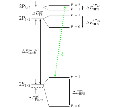
Figure 1: (Color online) Muonic hydrogen spectrum, including finite-size correction, Lamb shift, fine structure, and hyperfine structure. Also shown is the measured 2S${}_{1/2}^{F=1}$ to 2P${}_{3/2}^{F=2}$ transition (green, dotted, $\xi$) as per Ref. Pohl et al. (2010).

2 Numerical Method

To calculate the theoretical shift corresponding to the measured transition, previous authors have primarily used perturbation theory with non-relativistic wave-functions to predict the size of the contributing effects, including relativistic effects. To better approximate the exact energies, we can use the Dirac equation for the muon with the appropriate potential as an effective approximation to the two-particle Bethe-Saltpeter equation Eides et al. (2001) to calculate the perturbed wave-functions, expressed here as a spinor

$$\psi_{\alpha}(\vec{r\,})=\begin{pmatrix}g_{\alpha}(r)\chi_{\kappa}^{\mu}(\hat{r})\\[5.69054pt] -if_{\alpha}(r)\chi_{-\kappa}^{\mu}(\hat{r})\end{pmatrix}=\begin{pmatrix}{\displaystyle\frac{G_{\alpha}(r)}{r}}\ \chi_{\kappa}^{\mu}(\hat{r})\\[5.69054pt] {\displaystyle\frac{-iF_{\alpha}(r)}{r}}\ \chi_{-\kappa}^{\mu}(\hat{r})\end{pmatrix},$$ (1)

normalised to unity, such that the probability is

$$\int|\psi_{\alpha}|^{2}\;d^{3}r=\int_{0}^{\infty}r^{2}\left[g_{\alpha}(r)^{2}+f_{\alpha}(r)^{2}\right]\;dr=1,$$ (2)

noting that

$$\int\chi_{\kappa}^{m\dagger}\chi_{\kappa^{\prime}}^{m^{\prime}}\;d\hat{r}=\delta_{\kappa\kappa^{\prime}}\delta_{mm^{\prime}}.$$ (3)

Since this is a relativistic system, we use the reduced mass $\mu$ in place of the muon mass in the Dirac equation

$$\mu=\frac{M_{p}m_{\mu}}{M_{p}+m_{\mu}},$$ (4)

which along with the addition of recoil corrections provides a good approximation to the Bethe-Saltpeter equation. Since the binding of the muon in this system is extremely weak, the eigenvalue $\epsilon_{\alpha}$ for each state calculated using the Dirac equation is approximately equal to the reduced mass $\mu$. In order to precisely calculate the variance from this value, we shift our eigenvalue down by the reduced mass, such that the eigenvalue we are now solving for is $\lambda_{\alpha}=\epsilon_{\alpha}-\mu$, thus the effective Dirac equation is

$$\frac{d}{dr}\begin{pmatrix}G_{\alpha}(r)\\[5.69054pt] F_{\alpha}(r)\end{pmatrix}=\left(\begin{array}[]{cc}-{\displaystyle\frac{\kappa_{\alpha}}{r}}&\lambda_{\alpha}+2\mu-V(r)\\[5.69054pt] -\lambda_{\alpha}+V(r)&{\displaystyle\frac{\kappa_{\alpha}}{r}}\end{array}\right)\begin{pmatrix}G_{\alpha}(r)\\[5.69054pt] F_{\alpha}(r)\end{pmatrix},$$ (5)

where the value of $\kappa_{\alpha}$ is specific to each eigenstate, namely

$${\rm 1S}_{1/2}:\kappa= -1,\quad{\rm 2S}_{1/2}:\kappa= -1,$$

$${\rm 2P}_{1/2}:\kappa= +1,\quad{\rm 2P}_{3/2}:\kappa= -2.$$

The (shifted) eigenvalues can be reliably reproduced by using the point-Coulomb potential

$$V(r)=-\frac{Z\alpha}{r},$$ (6)

in Eq. (5). In order to integrate Eq. (5), we supply an initial guess for the eigenvalue $\lambda_{\alpha}$, and appropriate boundary behaviour of upper and lower components of the wave-function at small and large radii, then integrate from each limit towards a central match-point. The discontinuity in the wave-function integrated from each limit is used as a measure of the inaccuracy of the eigenvalue and a refined estimate is calculated. This process is iterated until the change in $\lambda_{\alpha}$ is less than the required tolerance, at which point we regard the wave-function to be converged.

To convince ourselves that our method is self-consistently accurate, we check the accuracy of our procedure using several methods. The unperturbed Dirac eigenvalues are known analytically Rafelski (1977) to be

$$\lambda_{\alpha}=\epsilon_{\alpha}-\mu=\mu\left[1+\frac{Z^{2}\alpha^{2}}{\left(n_{\alpha}-|\kappa_{\alpha}|+\sqrt{\kappa_{\alpha}^{2}-Z^{2}\alpha^{2}}\right)^{2}}\right]^{-\frac{1}{2}}-\mu,$$ (7)

where $n_{\alpha}$ is the principle quantum number for the state $\alpha$. We first ensure that we are able to reproduce these values. For the 2S_1/2 wave-function, we reproduce this value to within 0.01 $\mu$eV using quad-precision Fortran, a sufficiently large grid size, and sufficiently small grid spacing, within reasonable compute-time. We also check the validity of the virial theorem for our solutions (refer to Ref. Rafelski (1977) for further details) by calculating the reduced eigenvalue as

$$\lambda=\langle{\rm 2S}_{1/2}\,|\,\mu\beta+V(\vec{r\,})+\vec{r\,}\cdot\vec{\nabla}V(\vec{\,r})\,|\,{\rm 2S}_{1/2}\rangle-\mu,$$ (8)

which tests the accuracy of the wave-function at the origin where $|\vec{\nabla}V|$ is greatest. We calculate that the values obtained using Eqs. (7) and (8) differ by 0.18 $\mu$eV for a point-Coulomb potential, and 0.45 $\mu$eV a finite-Coulomb potential (to be discussed later). We therefore conservatively take our errors to be of the order of $\sim\pm 0.5$ $\mu$eV.

3 Numerical Calculations

$\bullet$ 2S_1/2–2P_1/2 Lamb Shift: The Lamb shift is the splitting of the otherwise degenerate 2S_1/2 and 2P_1/2 eigenstates attributed to the vacuum polarization potential $V_{\rm VP}$

$$V_{\rm VP}(r)=-\frac{Z\alpha}{r}\frac{\alpha}{3\pi}\int_{4}^{\infty}\frac{e^{-m_{e}qr}}{q^{2}}\ \sqrt{1-\frac{4}{q^{2}}}\left(1+\frac{2}{q^{2}}\right)d(q^{2}).$$ (9)

We can calculate the shift in eigenvalues using converged Dirac wave-functions in response to the Coulomb and vacuum polarization potentials, and in this case we simply take the difference between the converged eigenvalues for the 2S_1/2 and 2P_1/2 states

$$\Delta E_{\rm Lamb}^{\rm 2S-2P}=\lambda_{\rm 2P_{1/2}}-\lambda_{\rm 2S_{1/2}}=205.1822~{}{\rm meV}.$$ (10)

Care must be taken when comparing this calculation to that of perturbative results since our calculation includes relativistic corrections, which are included later as corrections in perturbative calculations, e.g. Ref. Borie (2005).

$\bullet$ Proton Finite-Size Corrections: To calculate this effect in our fully relativistic calculation, we consider the replacement of the point-Coulomb potential with the finite-size Coulomb potential in Eq. (5)

$$V_{C}(r)=-\frac{Z\alpha}{r}\to-Z\alpha\int\frac{\rho(r^{\prime})}{|\vec{r}-\vec{r\,}^{\prime}|}d^{3}r,$$ (11)

where $\rho(r)$ is the proton charge-distribution (or more accurately, the slope of the electric form-factor). We have studied the dependence of the finite-size correction on the form of this term (always normalised to unity) and this will be summarized in an upcoming publication (Ref. Carroll et al. (2011b)), though the dependence on the choice of charge-distribution — whether it be exponential, Yukawa, or Gaussian in form — appears to be small. Similarly the finite vacuum polarization potential is given by a convolution of Eq. (9) with the charge-distribution.

The exponential form for the charge-distribution, normalised to unity such that ${\int\rho(r)\,d^{3}r=1}$ is given by

$$\rho(r)=\frac{\eta}{8\pi}e^{-\eta r};\quad\eta=\sqrt{12/\langle r_{p}^{2}\rangle}.$$ (12)

We calculate the Lamb shift by taking the difference between the appropriate eigenvalues calculated using the Dirac equation with the potential given by Eq. (11) with the charge-distribution given by Eq. (12) for various values of $\langle r_{p}^{2}\rangle$. We then interpolate the energy shifts and fit the data to a cubic of the form

$$f(x)=A+B\langle r_{p}^{2}\rangle+C\langle r_{p}^{2}\rangle^{3/2},$$ (13)

which provides the relevant parameterization. The dependence of the Lamb shift on the rms charge radius in the presence of an exponential finite-sized Coulomb potential and finite vacuum polarization potential is given by

$$\Delta E_{\rm finite}=205.1822-5.2519\langle r_{p}^{2}\rangle+0.0546\langle r_{p}^{2}\rangle^{3/2}~{}{\rm meV}.$$ (14)

$\bullet$ 2P Fine Structure: Subtracting the converged eigenvalues of the 2P_1/2 and 2P_3/2 eigenstates gives the fine structure splitting

$$\Delta E_{FS}^{2P}=\lambda_{2P_{3/2}}-\lambda_{2P_{1/2}}$$ (15)

which we can also calculate in the presence of the various potentials. For the case of an exponential finite-Coulomb potential with finite vacuum polarization potential, the 2P fine structure shift is

$$\Delta E_{FS}^{\rm 2P}=8.4206(5)~{}{\rm meV}.$$ (16)

The shifts due to finite-size effects (as compared to the point cases) are below the level of errors for our calculation. The point vacuum polarization itself increases the fine structure shift by $5~{}\mu$eV.

$\bullet$ 2S_1/2 Hyperfine Structure: The splitting between the 2S $F=0$ and $F=1$ hyperfine eigenvalues is given Weissbluth (1978) by

$$\Delta E_{HFS}^{2S(F=1-F=0)}=\frac{16\pi}{3}\beta\gamma|\psi(0)|^{2}.$$ (17)

The value of the 2S hyperfine shift, as calculated using Eq. (17) with the wave-function calculated with the Dirac equation in the presence of the combined point-Coulomb and point vacuum polarization potentials is

$$\Delta E_{HFS}^{2S}=22.8967(5)~{}{\rm meV}.$$ (18)

The finite-size effects will be investigated in an upcoming publication Carroll et al. (2011a).

$\bullet$ 2P_1/2 Hyperfine Structure: The 2P_1/2 Hyperfine structure is of no consequence to the measured transition we are investigating. Nonetheless, we calculate the energy of the 2P${}_{1/2}^{F=0}$ and 2P${}_{1/2}^{F=1}$ states as a confirmation of our method, and to compare to perturbative results. The 2P hyperfine structure is given Weissbluth (1978) by

$$E_{\rm HFS}^{{\rm 2P}}=2\beta\gamma\frac{\ell(\ell+1)}{j(j+1)}\bigg{\langle}\frac{1}{r^{3}}\bigg{\rangle}\langle Fm_{F}\,|\,\mathbf{I}\cdot\mathbf{J}\,|\,Fm_{F}\rangle,$$ (19)

where the non-zero terms in the dot-product are given by

$$\langle Fm_{F}\,|\,\mathbf{I}\cdot\mathbf{J}\,|\,Fm_{F}\rangle=\frac{1}{2}[F(F+1)-I(I+1)-j(j+1)],$$ (20)

which, for Schrödinger wave-functions gives

$$\Delta E_{\rm HFS}^{{\rm 2P}_{1/2}}=\frac{2}{9}\beta\gamma/a_{0}^{3}\ ,$$ (21)

to which anomalous magnetic moments provide further corrections. Using the converged Dirac wave-functions with exponential finite-Coulomb and finite vacuum polarization potentials (rather than Schrödinger wave-functions) we calculate the expectation value of $r^{-3}$ and find

$$\Delta E_{\rm HFS}^{{\rm 2P}_{1/2}}=7.6204(5)~{}{\rm meV}.$$ (22)

The addition of the (point) vacuum polarization potential to the point-Coulomb potential increases the splitting by 0.0017(5) meV, and the introduction of the finite-Coulomb potential increases this further by 0.0045(5) meV. The finite vacuum polarization potential does not alter the result from the point case here.

$\bullet$ 2P_3/2 Hyperfine Structure: Following the same method as the 2P_1/2 calculation, we can calculate the energy levels for the 2P${}_{3/2}^{F=1}$ and 2P${}_{3/2}^{F=2}$ eigenstates. Using the converged Dirac wave-functions we find

$$\Delta E_{\rm HFS}^{{\rm 2P}_{3/2}}=3.0415(5)~{}{\rm meV}$$ (23)

when the potential consists of the exponential finite-Coulomb and finite vacuum polarization potentials. For this state, the addition of the (point) vacuum polarization potential to the point-Coulomb potential increases the splitting by 0.0007(5) meV, and the introduction of the finite-size effects was found to make no change within the limits of our calculation.

4 Conclusions

We find that the Dirac calculations performed here agree well with perturbative results once appropriate corrections are made (taking care regarding double-counting of effects). The calculations presented here and discussions of the comparison to perturbative calculations will be fully detailed in several upcoming publications Carroll et al. (2011a, b).

References

- Pohl et al. (2010) R. Pohl, A. Antognini, F. Nez, F. D. Amaro, F. Biraben, et al., Nature 466, 213–216 (2010).
- Mohr et al. (2008) P. J. Mohr, B. N. Taylor, and D. B. Newell, Rev. Mod. Phys. 80, 633–730 (2008), 0801.0028.
- Carroll et al. (2011a) J. Carroll, A. W. Thomas, J. Rafelski, and G. A. Miller (2011a), (in preparation).
- Borie and Rinker (1982) E. Borie, and G. A. Rinker, Rev. Mod. Phys. 54, 67–118 (1982).
- Martynenko (2005) A. Martynenko, Phys.Rev. A71, 022506 (2005), hep-ph/0409107.
- Martynenko (2008) A. Martynenko, Phys.Atom.Nucl. 71, 125–135 (2008), hep-ph/0610226.
- Miller et al. (2011) G. A. Miller, A. W. Thomas, J. D. Carroll, and J. Rafelski (2011), 1101.4073.
- Eides et al. (2001) M. I. Eides, H. Grotch, and V. A. Shelyuto, Phys. Rept. 342, 63–261 (2001), hep-ph/0002158.
- Rafelski (1977) J. Rafelski, Phys. Rev. D16, 1890 (1977).
- Borie (2005) E. Borie, Phys. Rev. A 71, 032508 (2005).
- Carroll et al. (2011b) J. Carroll, A. W. Thomas, J. Rafelski, and G. A. Miller (2011b), (in preparation).
- Weissbluth (1978) M. Weissbluth, Atoms and molecules, Academic Press, 1978, ISBN 9780127444505.