Optimized pulses for the control of uncertain qubits

Abstract

Constructing high-fidelity control fields that are robust to control, system, and/or surrounding environment uncertainties is a crucial objective for quantum information processing. Using the two-state Landau-Zener model for illustrative simulations of a controlled qubit, we generate optimal controls for $\pi/2$- and $\pi$-pulses, and investigate their inherent robustness to uncertainty in the magnitude of the drift Hamiltonian. Next, we construct a quantum-control protocol to improve system-drift robustness by combining environment-decoupling pulse criteria and optimal control theory for unitary operations. By perturbatively expanding the unitary time-evolution operator for an open quantum system, previous analysis of environment-decoupling control pulses has calculated explicit control-field criteria to suppress environment-induced errors up to (but not including) third order from $\pi/2$- and $\pi$-pulses. We systematically integrate this criteria with optimal control theory, incorporating an estimate of the uncertain parameter, to produce improvements in gate fidelity and robustness, demonstrated via a numerical example based on double quantum dot qubits. For the qubit model used in this work, post facto analysis of the resulting controls suggests that realistic control-field fluctuations and noise may contribute just as significantly to gate errors as system and environment fluctuations.

I Introduction

Demanding requirements for gate fidelities to achieve fault-tolerant quantum computation (QC) Gaitan08a have motivated the need for improved quantum control protocols (QCPs). In quantum information science Ladd10a , there are (at least) three distinct dynamical approaches to improving the fidelity of qubit operations in the presence of environmental interactions: dynamical-decoupling (DD) pulse sequences Liu07a ; Uhrig08a , optimal control theory (OCT) Roloff09a ; Brif10a , and quantum error-correcting codes (QECCs) Gaitan08a . Although interesting non-dynamical methods exist for noise suppression, e.g., decoherence-free subspaces (DFSs) Lidar03a , noiseless subsystems Zanardi97a , and anyonic/topological systems Nayak08a , the work reported in this article focuses exclusively on dynamical approaches for controlling quantum systems Werschnik07a . Specifically, the objective of this work is to construct a hybrid QCP, combining methods and results from DD and OCT, to locate control fields that (a) produce high-fidelity rotations about a particular axis and (b) are robust with respect to an uncertain frequency of rotation about an orthogonal axis. By combining complementary features of these analytically- and numerically-based QCPs, we have developed a hybrid QCP where estimates of system parameters can be directly incorporated into numerical simulations to generate improved quantum operations.

During the past few years, P. Karbach, S. Pasini, G. Uhrig, and colleagues have made significant contributions toward the mathematical analysis and design of DD pulses and sequences for controlling qubit systems and decoupling them from their surrounding environment, e.g., refs. Uhrig07a ; Uhrig08a ; Karbach08a ; Pasini08a ; Pasini08b ; Pasini09a ; Pasini10a ; Pasini11a . In a recent article Pasini09a , using a rather general open-system, time-dependent Hamiltonian for one qubit, they derive analytical control-field criteria for $\pi/2$- and $\pi$-pulses, which, when satisfied, eliminate the first- and second-order errors in the unitary time-evolution operator resulting from qubit-environment interactions. In this work, we refer to these criteria as “decoupling-pulse criteria” (DPC) and to the control fields that satisfy this criteria as “decoupling pulses” (DPs). We adapt the DPC for the case of closed-system unitary control, where the dynamics are influenced by an uncertain drift (i.e., time-independent) term in the qubit Hamiltonian. For control fields that satisfy the DPC, this adaptation eliminates the first- and second-order effects resulting from the drift term. Using a novel method for multi-objective control, we combine the mathematical DPC with a numerical procedure based on OCT for unitary control Palao03a that incorporates an estimate of the drift-term magnitude (i.e., system information) to construct control fields with increased fidelity and robustness to uncertainty in the drift term. For brevity, we refer to this combination of the DPC and OCT as “DPC+OCT”. To demonstrate the utility of our approach, we optimize and evaluate these control fields using a qubit model based on the two-level Landau-Zener Hamiltonian Messiah99a that has an uncertain drift term and is driven by a deterministic control field. Even though the qubit model is quite general, i.e., the Hamiltonian employed represents a one-qubit system with a linear drift term, driven by a scalar control field, and thus describes a variety of qubits (e.g., atomic, spin, superconducting, etc. Ladd10a ), we select physical units for the model that are relevant to double quantum dot (DQD) qubits to investigate the practical features of our results Levy11a . With this model system, we demonstrate that the DPC+OCT combination can be used to produce (a) improved fidelity compared to DPs alone and (b) improved robustness to uncertainty in the drift magnitude compared to results from DPs and OCT alone. Although research examining the effects of classical control noise is extremely important for practical QC vanEnk02a ; Sola04a , all control fields in this work are assumed to be deterministic, with control amplitudes that are exact to numerical precision. Thus, uncertainty is assumed to be present only in the system, and, unless otherwise specified, control robustness refers to robustness to drift uncertainty.

Related research on hybrid QCPs includes that performed by Lidar et al., who proposed the application of DD pulse sequences on logical qubits encoded in DFSs or QECCs to eliminate decoherence in solid-state and trapped-ion qubits Byrd02b ; Byrd03a ; Khodjasteh03a ; Ng11a . Borneman et al. used OCT to design control fields that are robust to systematic amplitude and resonance inhomogeneities, thereby improving the performance of the so-called Carr-Purcell-Meiboom-Gill pulse sequence Borneman10a . In addition, there have been many studies on the control and controllability of (inhomogeneous) quantum-mechanical ensembles, such as a collection of coupled or uncoupled spin systems, primarily for state-based objectives, e.g., refs. Khaneja05a ; Li06b ; Dong09a ; Ruths10a ; Ruths11a , and sequences of unitary time-evolution operators that compensate for systematic off-resonant effects, e.g., Cummins00a ; Cummins03a ; Brown04a ; Alway07a ; Jones11a .

This article is organized as follows. Section II introduces and develops the model qubit system based on the Landau-Zener Hamiltonian Messiah99a used in our optimizations and simulations. For illustrative purposes, this model is compared to a logical DQD semiconductor qubit, where uncertainty in the drift term of the system Hamiltonian is due to the surrounding nuclear spin environment Witzel06a ; Witzel07a . A system of scaled units is defined that allows for the comparison of our model and control fields to relevant experimental parameters. In section III, we summarize our gradient-based OCT routine for deterministic Hamiltonian systems, describing our objective functional for unitary control, relevant control properties, and the numerical optimization procedure. Section IV presents results from unitary OCT for subsequent comparison to those from the DPC and DPC+OCT QCPs. Inherent robustness of these optimal controls (OCs) to variations in the magnitude of the uncertain drift term is also analyzed, and a functional is proposed to quantify this robustness. For the individual unitary targets considered, despite the similar structures of the resulting OCs for different drift-term magnitudes, their gate distances as a function of the drift magnitude differ dramatically. Section V summarizes the nonlinear control-field criteria developed by Pasini et al. for designing control pulses that are robust to decoherence Pasini09a . Our adaptation of these criteria to closed-system unitary control is explained and the hybrid DPC+OCT control problem is posed. Control fields satisfying this criteria are applied to our model qubit system and their robustness is analyzed. In section VI, we describe and mathematically formulate our gradient-based method for solving the nonlinearly-constrained control problem. Section VII presents results from our DPC+OCT optimization algorithm. Gate distance and robustness of the control fields are numerically analyzed and discussed. We also compare OCT, DPC, and DPC+OCT results collectively to illustrate the benefit of our hybrid approach. In addition to comparing the gate distances directly, we apply these controls to an inhomogeneous ensemble of systems to emphasize the improvement that may be obtained from this hybrid QCP. Like the OCT results, significant gate-distance sensitivities to relatively small control-field differences are observed for the DPC+OCT controls, supporting further study and suppression of the effects of undesired control-field fluctuations and noise on quantum information processing. We conclude this article in section VIII with a summary of our results and identify several future directions of our research.

II Landau-Zener model system

II.1 Model Hamiltonian

We represent the dynamical model of a qubit with the following Hamiltonian (where $\hbar=1$; details regarding units appear in section II.3):

$$H(t):=\varepsilon S_{x}+C(t)S_{z},$$ (1)

where $S_{\lambda}:=\sigma_{\lambda}/2$ is a spin operator for a spin-$1/2$ particle, $\sigma_{\lambda}$ is a Pauli matrix $\left(\lambda\in\{x,y,z\}\right)$, $\varepsilon S_{x}$ represents a persistent rotation about the $x$-axis, and $C(t)$ represents the time-dependent control field driving rotations about the $z$-axis. Note that $H(t)$ corresponds to the two-state Landau-Zener model Messiah99a , and that both $C(t)/\hbar$ and $\varepsilon/\hbar$ have units of angular frequency, e.g., radians per second in SI units.

Let $\mathcal{H}$ denote the Hilbert space of the system, where $n:=\dim\{\mathcal{H}\}$ ($n=2$ for one qubit), and $\left\{|\mathcal{S}_{i}\rangle\right\}$ denote the orthonormal basis of $S_{z}$ that spans $\mathcal{H}$, with corresponding eigenvalues $\pm 1/2$. The Lie group of all unitary operators on $\mathcal{H}$ is denoted by $\mathrm{U}(\mathcal{H})$. In general, the unitary time-evolution operator $U(t)\in\mathrm{U}(\mathcal{H})$ for a closed quantum system obeys the time-dependent Schrödinger equation:

$$\dot{U}(t)=-\mathrm{i}H(t)U(t),$$ (2)

where $U(t=0)=\openone_{n}$, the $n\times n$ identity matrix. From a controllability perspective Huang83a ; Rama95a , the Hamiltonian in eq. (1) generates the Lie algebra $\mathrm{su}(2)$. Thus, the system is completely dynamically controllable, i.e., any element of the Lie group $\mathrm{SU}(2)$ can be generated via eq. (2) and an appropriately-shaped control field. However, this analysis does not necessarily reveal anything about the control-field structure required to realize an arbitrary $\mathrm{SU}(2)$ operation. As an illustrative example of our DPC+OCT QCP, we focus on constructing unitary operations corresponding to $\pi/2$- and $\pi$-rotations about the $z$-axis.

II.2 Double quantum dot logical qubit

Although our qubit model is quite general, for illustrative purposes we refer to a particular application of a DQD solid-state qubit Hanson07a ; Taylor07a , which has been studied in an array of experiments, e.g., Johnson05a ; Petta05a ; Petta08a ; Foletti09a ; Bluhm10a . With one electron in each quantum dot, the DQD system spans four spin-1/2 states. An applied magnetic field will break the degeneracy of the states in which both electrons are either aligned against or with the field. In this situation, it is possible (and often advantageous) to work within the two-level subspace where the net spin angular momentum is zero. By adjusting voltages in the electrostatically defined quantum dots, the magnitude of the exchange interaction between the electrons may be controlled. This interaction controls the splitting between the singlet, $\lvert S\rangle:=(\lvert\uparrow\downarrow\rangle-\lvert\downarrow\uparrow\rangle)/\sqrt{2}$ and triplet, $\lvert T_{0}\rangle:=(\lvert\uparrow\downarrow\rangle+\lvert\downarrow\uparrow\rangle)/\sqrt{2}$, states of the spin-zero manifold. Designating $|\mathcal{S}_{0}\rangle=|S\rangle$ and $|\mathcal{S}_{1}\rangle=|T_{0}\rangle$, we equate $C(t)$ in our general model [eq. 1] with the exchange interaction.

The spin-zero manifold is insensitive to a global magnetic field. However, gradients in the magnetic field will cause singlet-triplet transitions. Such a gradient splits the energy of the states $\lvert\uparrow\downarrow\rangle=(\lvert T_{0}\rangle+\lvert S\rangle)/\sqrt{2}$ and $\lvert\downarrow\uparrow\rangle=(\lvert T_{0}\rangle-\lvert S\rangle)/\sqrt{2}$ by the difference in effective Zeeman energies for an electron in either of the two quantum dots. In this context, we may therefore equate the energy $\varepsilon$ with this effective Zeeman energy difference. In GaAs DQD systems, the effective Zeeman energy difference is typically dominated by the Overhauser shifts from a lattice of randomly polarized nuclear spins corresponding to approximately $1.602\times 10^{-26}$ – $1.602\times 10^{-25}$ J (or $10^{-7}$ – $10^{-6}$ eV) Hanson07a ; Taylor07a . It has been demonstrated that a desired difference in Overhauser shift of a GaAs DQD may be realized through feedback control from a preparatory qubit Bluhm10a . However, the value of $\varepsilon$ will drift over time through the nuclear spin diffusion that causes spectral diffusion Witzel06a ; Witzel07a ; Yao06a ; Liu07a , motivating the need for robust control. In proposed Si DQD systems, e.g., ref. Levy09a , nuclear spins may be eliminated through isotopic enrichment. Other spin baths, such as electron spins of donor impurities Witzel10a or dangling bond spins at an interface deSousa07a , may also lead to variations and drift in the value of $\varepsilon$.

II.3 Scaled unit system

In addition to setting the reduced Planck constant $\hbar=1$ (corresponding to unit of angular momentum: energy $\times$ time), a simple set of scaled units is defined by also setting the final time of the controlled evolution $t_{\mathrm{f}}=1$. The ratio $\hbar/t_{\mathrm{f}}=1$ yields the scaled unit of energy, which, when $t_{\mathrm{f}}=20$ ns (as an example), corresponds to approximately $5.273\times 10^{-27}$ J (or $3.291\times 10^{-8}$ eV). By appropriately scaling the Hamiltonian and control field, this propagation time can be transformed to any final time $t_{\mathrm{f}}$. Relationships between these scaled units and SI units (when $t_{\mathrm{f}}=20$ ns) are summarized in table 1.

In this work, optimizations were performed for individual values of $\varepsilon\in[0,5]$; we denote the nominal values of $\varepsilon$ used in these calculations as $\varepsilon_{0}$. This range of $\varepsilon$ corresponds to no and moderate rotations from the environment for the GaAS DQD example. For a DQD logical qubit,

$$\varepsilon=g_{\mathrm{e}}\mu_{\mathrm{B}}B_{\!\Delta},$$ (3)

where $g_{\mathrm{e}}$ is the so-called electron $g$-factor, $\mu_{\mathrm{B}}$ is the Bohr magneton, and $B_{\!\Delta}$ is the magnetic field resulting from the difference in the random hyperfine fields from each quantum dot along the direction of the applied field. When 1 scaled unit of time corresponds to 20 ns (a representative estimate of the time required for one-qubit rotations for a DQD system Petta05a ; Petta10a ), $\varepsilon=5$ scaled units of angular frequency (the maximum value of $\varepsilon_{0}$ considered) corresponds to $B_{\!\Delta}\approx 6.5$ mT; this is consistent with experimental reports of GaAs DQDs (where $g_{\mathrm{e}}=-0.44$) Petta05a ; Hanson07a ; Taylor07a . Unless stated otherwise, all physical quantities in this work are expressed in scaled units.

Physical quantity	Scaled unit	SI unit
angular momentum: $\hbar$	1	$1.055\times 10^{-34}$ J s
time: $t$	1	$2.0\times 10^{-8}$ s
energy: $C$, $\varepsilon$	1	$5.273\times 10^{-27}$ J

Table 1: Scaled and SI units for the logical qubit described by the Hamiltonian in eq. (1).

III Optimal control of unitary operations via gradient-based algorithms

III.1 Objective functionals for unitary operations

For a target unitary operation $V\in\mathrm{U}(\mathcal{H})$, the distance $\Delta$ between $V$ and a simulated final-time unitary operation $U(t_{\mathrm{f}})$ is

$$\Delta[V,U(t_{\mathrm{f}};C)] :=\min_{\varphi\in\mathbb{R}}\frac{1}{\sqrt{2n}}\left\|U(t_{\mathrm{f}};C)-\exp(\mathrm{i}\varphi)V\right\|_{\mathrm{HS}},$$ (4a)

$$=\sqrt{1-\frac{1}{n}\left|\mathrm{Tr}\left[V^{{\dagger}}U(t_{\mathrm{f}})\right]\right|},$$ (4b)

where $\|\cdot\|_{\mathrm{HS}}$ denotes the norm based on the Hilbert-Schmidt inner product: $\langle A,B\rangle_{\mathrm{HS}}:=\mathrm{Tr}(A^{{\dagger}}B)$, $A,B\in\mathcal{M}_{n}(\mathbb{C})$ [$\mathcal{M}_{n}\left(\mathbb{X}\right)$ denotes the set of $n\times n$ matrices over the field $\mathbb{X}$]. This phase-invariant distance measure is a special case of a more general distance measure developed in ref. Grace10a , which is applicable to studies involving composite systems where only the qubit/system dynamics are directly of interest Grace07a ; Grace07b .

Concerning mathematical notation, because the unitary time-evolution operator is a function of time and a functional of the control, it will be expressed more generally as $U(t;C)$ for all time $t$ and a control $C$, compared to $U(t)$; the final-time unitary operator will be expressed more generally as $U_{t_{\mathrm{f}}}(C)$, compared to $U(t_{\mathrm{f}})$. Also, we denote the space of admissible controls with final time $t=t_{\mathrm{f}}$ as $\mathfrak{C}_{t_{\mathrm{f}}}$. Some properties of the Hilbert space $\mathfrak{C}_{t_{\mathrm{f}}}$ are discussed below; further details are in ref. Grace10a .

Because $0\leq\Delta\leq 1$ in general, it is useful to define the fidelity $\mathcal{F}$ of unitary operations as Fuchs99a ; Grace10a

$$\mathcal{F}:=\frac{1}{n}\left|\mathrm{Tr}\left[V^{{\dagger}}U(t_{\mathrm{f}})\right]\right|=1-\Delta^{2}(V,U_{t_{\mathrm{f}}}),$$ (5)

which is a common phase-invariant measure of gate fidelity based on the Hilbert-Schmidt inner product, e.g., refs. Palao03a ; Dominy08a ; Ho09a . Note the quadratic dependence of $\mathcal{F}$ on $\Delta$, i.e., a distance of $10^{x}$ corresponds to a fidelity of $1-10^{2x}$, where $x\leq 0$.

An optimal control field for a given unitary operation may be located by minimizing an objective functional $\mathcal{J}[C]$ of the control field that incorporates the final-time unitary target $V$, constrains the dynamics of $U(t)$ to evolve according to eq. (2), and penalizes the fluence of the control field. For this work, the objective functional is defined as

$$\mathcal{J}[C]:=\Delta[V,U_{t_{\mathrm{f}}}(C)]+\frac{\alpha}{2}\int_{0}^{t_{\mathrm{f}}}\!\frac{C^{2}(t)}{s(t)}\mathrm{d}t.$$ (6)

Often, the minimization of $\mathcal{J}$ is performed using a gradient-based algorithm (GrA; see Palao03a ; Grace07a ; Balint08a ; Grace10a for details and examples of gradient-based optimizations). Here, $\alpha\geq 0$ weighs the control-field fluence relative to the distance $\Delta$ and $s:[0,t_{\mathrm{f}}]\mapsto\mathbb{R}$ is a continuous “shape function”. When appropriately chosen, $s(t)$ penalizes undesirably-shaped functions Grace10a . We use $s(t)=\sin^{p}(\pi t/t_{\mathrm{f}})$, where $p\in\mathbb{Q}_{+}\cup\{0\}$. For $p\neq 0$, this form penalizes the control-field slew rate around the initial and final times and favors controls where $C(0)=C(t_{\mathrm{f}})=0$.

For the time-dependent Hamiltonian in eq. (1), $U_{t_{\mathrm{f}}}:\mathfrak{C}_{t_{\mathrm{f}}}\to\mathrm{U}(\mathcal{H})$ denotes the map, defined implicitly through the Schrödinger equation [eq. (2)], that takes a control field $C\in\mathfrak{C}_{t_{\mathrm{f}}}$ to the final-time unitary evolution operator $U_{t_{\mathrm{f}}}\in\mathrm{U}(\mathcal{H})$. Note that $\mathfrak{C}_{t_{\mathrm{f}}}$ is a Hilbert space of admissible controls, on which $U(t;C)$ exists for all $t\in[0,t_{\mathrm{f}}]$ and all $C\in\mathfrak{C}_{t_{\mathrm{f}}}$ Jurdjevic72a , where the inner product on $\mathfrak{C}_{t_{\mathrm{f}}}$ is

$$\langle f,g\rangle_{\mathfrak{C}_{t_{\mathrm{f}}}}:=\int_{0}^{t_{\mathrm{f}}}\!\frac{f(t)g(t)}{s(t)}\mathrm{d}t,\ \ \forall f,g\in\mathfrak{C}_{t_{\mathrm{f}}}.$$ (7)

As such, $\mathcal{J}:\mathfrak{C}_{t_{\mathrm{f}}}\to\mathbb{R}$ is the dynamical version of the distance measure $\Delta$, with a relative cost on the control-field fluence, determined by $\alpha$. The role of the shape function $s(t)$ in eqs. (6) and (7) is to change the geometry of control space, moving undesirably-shaped functions away from the origin, out to infinity, where they are less likely to be the targets of a minimization over $\mathfrak{C}_{t_{\mathrm{f}}}$ Grace10a .

III.2 Control rotation angle $\bm{\theta(t;C)}$

In addition to the objective functional $\mathcal{J}$ and inner product on $\mathfrak{C}_{t_{\mathrm{f}}}$, another important expression is the integral of the control field:

$$\theta(t;C):=\int_{0}^{t}\!C(\tau)\mathrm{d}\tau.$$ (8a)

The angle $$\theta z [0,t] \theta C(t) \theta(t;C) \theta(t)$$ corresponds to the rotation about the -axis performed by the control field during the time interval . Although is a functional of the control field , whenever appropriate we abbreviate as to avoid unnecessarily cumbersome notation. Equation (8a) is equivalent to

$$\frac{\mathrm{d}\theta(t;C)}{\mathrm{d}t}=C(t).$$ (8b)

Also,

$$\frac{\delta\theta[t;C]}{\delta C(t^{\prime})}=\mathfrak{H}(t-t^{\prime}),$$ (8c)

(i.e., the functional derivative of $\theta$ with respect to $C$) where $\mathfrak{H}(t-t^{\prime})$ is the Heaviside step function:

$$\mathfrak{H}(t^{\prime}-t):=\left\{\begin{array}[]{cc}1&\textrm{when}\ t\geq t^{\prime}\\ 0&\textrm{when}\ t<t^{\prime}\end{array}\right..$$ (9)

III.3 Optimization with a gradient-based algorithms

This section briefly summarizes the variational analysis of $\mathcal{J}$ and describes criteria for the optimal points (or submanifolds) of $\mathcal{J}$ with respect to a control field $C$. The gradient of the objective functional $\mathcal{J}$ is explicitly derived in ref. Grace10a ; we present it here for continuity:

$$\big{(}\nabla\mathcal{J}[C]\big{)}(t)=\frac{s(t)}{4n\,\Delta[V,U_{t_{\mathrm{f}}}(C)]}\mathrm{Im}\Big{(}\mathrm{Tr}\Big{\{}\big{[}U_{t_{\mathrm{f}}}^{{\dagger}}(C)R-R^{{\dagger}}U_{t_{\mathrm{f}}}(C)\big{]}U^{{\dagger}}(t;C)S_{z}U(t;C)\Big{\}}\Big{)}+\alpha C(t),$$ (10)

where $R:=\exp(\mathrm{i}\varphi)V$ and $\varphi:=\mathrm{Im}\left\{\ln\left[\mathrm{Tr}\left(V^{{\dagger}}U_{t_{\mathrm{f}}}\right)\right]\right\}$. Critical points of $\mathcal{J}$ (a real-valued functional) are defined as controls for which $\big{(}\nabla\mathcal{J}[C]\big{)}(t)=0$ for all time $t$ Brif12a . Control fields are iteratively updated using this gradient to improve the value of the objective functional $\mathcal{J}$. Given the $k$th iterate of the control field $C^{(k)}(t)$, adjustments to the control field for the $(k\!+\!1)$th iteration are given by

$$C^{(k+1)}(t):=C^{(k)}(t)-\beta\left(\nabla\mathcal{J}\left[C^{(k)}\right]\right)(t),$$ (11)

where $\beta$ is a constant that determines the magnitude of the field adjustment. This procedure describes an implementation of a steepest-descent algorithm Press92a . In this work, initial control fields $C^{(0)}$ are continuous approximations to simple square-wave pulses, where initial and final times and slew rates are consistent with the shape function $s(t)=\sin(\pi t/t_{\mathrm{f}})$.

IV Results from quantum optimal control theory

Using only the GrA presented in section III, OCs were found for unitary targets that perform $\pi/2$- and $\pi$-rotations about the $z$-axis:

$$Z_{\phi}:=\left(\begin{array}[]{cc}\exp\left(-\mathrm{i}\phi/2\right)&0\\ 0&\exp\left(\mathrm{i}\phi/2\right)\end{array}\right),$$ (12)

where $\phi\in\{\pi/2,\pi\}$. The final time for all OCs was fixed at $t_{\mathrm{f}}=1$ scaled unit of time. With the GrA and the objective functional $\mathcal{J}$, a combination of the value of $\varepsilon$ and the structure of the initial control field determines the resulting optimal control field. Optimizations were performed individually for specific angular frequencies: $\varepsilon_{0}\in[0,5]$. As described in section II.3, this interval represents the regime of zero to moderate rotation from the environment for the DQD logical qubit. To emphasize the $\varepsilon$-specific nature of these OCs, we denote them as $C_{\mathrm{o}}(\varepsilon_{0};t)$.

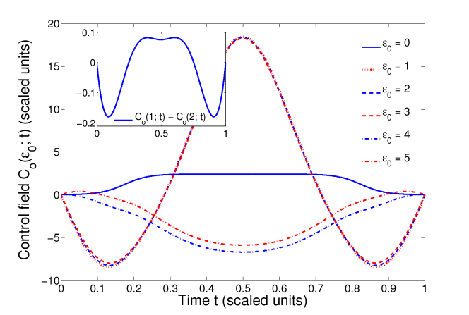
Figure 1: (Color online) OC fields producing a $Z_{\pi/2}$ operation for several specific values of $\varepsilon_{0}$ and $t_{\mathrm{f}}=1$ scaled unit. All OCs have distances $\Delta(Z_{\pi/2},U_{t_{\mathrm{f}}})\leq 10^{-6}$. The inset presents the difference between $C_{\mathrm{o}}(1;t)$ and $C_{\mathrm{o}}(2;t)$. Although distinct, note that $C_{\mathrm{o}}(1;t)$, $C_{\mathrm{o}}(2;t)$, and $C_{\mathrm{o}}(3;t)$ appear nearly indistinguishable in this figure.

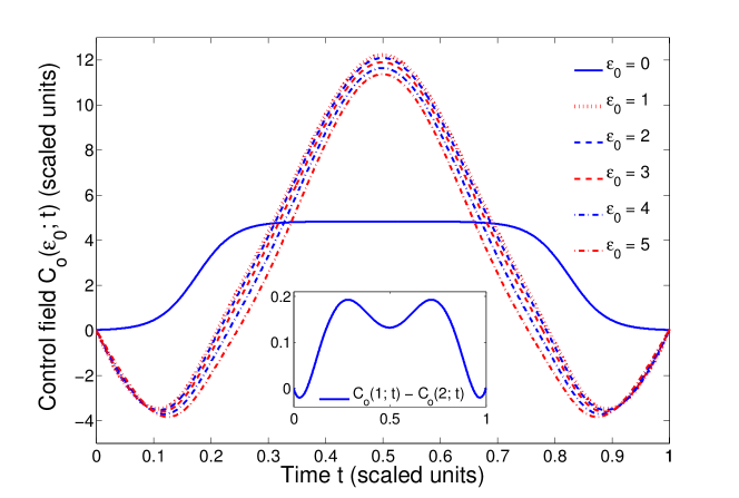
Figure 2: (Color online) OC fields producing a $Z_{\pi}$ operation for several specific values of $\varepsilon_{0}$ and $t_{\mathrm{f}}=1$ scaled unit. All OCs have distances $\Delta(Z_{\pi},U_{t_{\mathrm{f}}})<10^{-6}$. The inset presents the difference between $C_{\mathrm{o}}(1;t)$ and $C_{\mathrm{o}}(2;t)$.

Because of the similarity of results over the entire interval $0\leq\varepsilon\leq 5$, only a subset will be presented. OC fields for $Z_{\pi/2}$ and $Z_{\pi}$ as a function of $\varepsilon$ are presented in figs. 1 and 2, respectively, for $\varepsilon_{0}\in\{0,1,2,3,4,5\}$. Even though all of these OCs were located using the same initial control field, which is very similar to the OC reported for $\varepsilon_{0}=0$ for both targets, some of the converged fields differ dramatically for different values of $\varepsilon_{0}$. All OCs have distances $\Delta<10^{-6}$ (or $\mathcal{F}>1-10^{-12}$, essentially corresponding to the limits of numerical precision), which is expected because this system is relatively simple and fully controllable Huang83a ; Rama95a . For $\varepsilon_{0}=0$, all OCs for $Z_{\phi}$ satisfy $\theta(t_{\mathrm{f}})\equiv\phi\!\pmod{2\pi}$, i.e., OC design simply corresponds to pulse-area control in this situation. However, when $\varepsilon\neq 0$, there is no corresponding pulse-area requirement. In fact, if $\varepsilon$ is known accurately, it is possible to perform $Z_{\phi}$ operations with piecewise constant controls that satisfy $\theta(t_{\mathrm{f}})=0$. Table 2 contains information about some of the properties of these OCs. For a DQD logical qubit, we observe that these controls require negative exchange coupling values. Although negative exchange energy is uncommon, it is predicted to be possible to produce through combined tuning of the magnetic field, dot size, and tunnel coupling Nielsen10a .

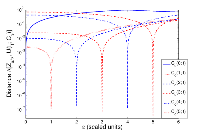
Figure 3: (Color online) Distance of OCs optimized with particular values of epsilon, denoted as $C_{\mathrm{o}}(\varepsilon_{0};t)$, for the $Z_{\pi/2}$ operation [$\Delta(Z_{\pi/2},U_{t_{\mathrm{f}}})<10^{-6}$ for all controls], subsequently applied over the interval $0\leq\varepsilon\leq 6$ (with a resolution of 0.01 scaled units).

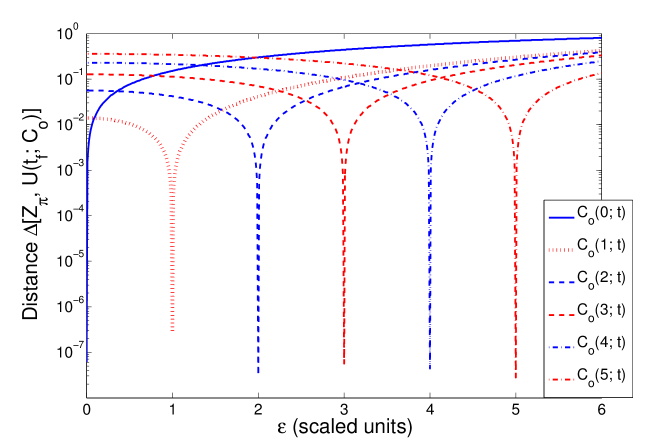
Figure 4: (Color online) Distance of OCs optimized with particular values of epsilon, denoted as $C_{\mathrm{o}}(\varepsilon_{0};t)$, for the $Z_{\pi}$ operation [$\Delta(Z_{\pi},U_{t_{\mathrm{f}}})<10^{-6}$ for all controls], subsequently applied over the interval $0\leq\varepsilon\leq 6$ (with a resolution of 0.01 scaled units).

For both $Z_{\pi/2}$ and $Z_{\pi}$ operations, despite the similar structures of the OCs, especially $C_{\mathrm{o}}(1;t)$ and $C_{\mathrm{o}}(2;t)$, their gate-distance responses for $0\leq\varepsilon\leq 6$ (with a numerical resolution of 0.01 scaled units) are quite unique, as shown in figs. 3 and 4, respectively. Even though $\max_{t}\left|C_{\mathrm{o}}(1;t)-C_{\mathrm{o}}(2;t)\right|<0.2$ scaled units of energy for both operations (see inset of figs. 1 and 2), and the mean relative difference is approximately 1.4% and 5.7% for the $Z_{\pi/2}$ and $Z_{\pi}$ operations, respectively, this two-level system effectively discriminates between these two similar control fields through the response of the distance functional $\Delta$ in eq. (4). Within the interval $0\leq\varepsilon\leq 3$, the gate distances of $C_{\mathrm{o}}(1;t)$ and $C_{\mathrm{o}}(2;t)$ do not significantly overlap. The sensitivity of this system to these relatively small control-field variations combined with the inherent noise (and limited resolution) present in most realistic control sources warrants further study of the impact that realistic control-field fluctuations may have on practical fault-tolerant QC Rabitz04a ; Dominy08a ; Levy09a ; Levy11a .

For the target operation $Z_{\pi/2}$, when $\varepsilon_{0}\in\{0,1,2,3\}$, the OCs produce a net positive angle of rotation about the $z$-axis, given the initial control field. When $\varepsilon_{0}\in\{4,5\}$, OCs produce a net negative angle of rotation about the $z$-axis. As the static angular frequency of the rotation about the $x$-axis increases, the OC strategy tends toward a controlled rotation about the $z$-axis in the negative direction. OC simulations for $3\leq\varepsilon_{0}\leq 4$, with a numerical resolution of 0.01 scaled units of energy (detailed results are not reported), reveal a distinct transition between OCs with shapes very similar to $C_{\mathrm{o}}(3,t)$ and $C_{\mathrm{o}}(4,t)$ reported in fig. 1, corresponding to net positive and negative rotations, respectively. For the initial control field used in this work, this transition occurs when $\varepsilon_{0}\approx 3.9$. Comparing the gate-distance responses in fig. 3 for $C_{\mathrm{o}}(3,t)$ and $C_{\mathrm{o}}(4,t)$ reveals that these OCs are not equivalent solutions for unitary control; the difference between these controls is exclusively due to the effect of the different values of $\varepsilon_{0}$ on the qubit dynamics.

Quantum-computing architectures often assume encoded quantum operations to correct the inevitable errors due to control and environmental noise. Gate operations, such as $Z_{\phi}$ simulated here, must achieve a minimum fidelity threshold for successful quantum error correction. A predicted maximum distance $\Delta$ of less than $10^{-3}$ for $\varepsilon\in[0,5]$ is within typical ranges necessary for fault-tolerant QC Taylor07a ; Gaitan08a ; Levy09a . These results highlight the potential advantage of using OCT if estimates of Hamiltonian parameters are known well. However, these OCs are not robust to uncertainty in the magnitude of $\varepsilon$; in fact, they are highly sensitive to small perturbatives in $\varepsilon$. Uncertainty can result from incomplete or poor system parameter estimates as well as from dynamics of the environment Witzel06a ; Witzel10a .

The objective functional $\mathcal{J}$ in eq. (6) does not include criteria to evaluate control-field robustness with respect to variations in $\varepsilon$. To investigate any inherent robustness quantitatively, OC fields optimized for particular values of $\varepsilon$ [i.e., $C_{\mathrm{o}}(\varepsilon_{0};t)$] were subsequently applied to a surrounding interval of $\varepsilon_{0}$. Results are presented in figs. 3 and 4 for the $Z_{\pi/2}$ and $Z_{\pi}$ operations, respectively. Consider the distance response of $C_{\mathrm{o}}(2;t)$ to variations in $\varepsilon$, which varies substantially with respect to variations that correspond to $\sim\!\!1$ mT fluctuations (corresponding to approximately $1.6\leq\varepsilon\leq 2.4$) for GaAS DQD systems. Without specifying a measure of robustness as an additional control objective, the resulting OCs are not inherently robust to modest local magnetic-field fluctuations (e.g., at each quantum dot). Numerical calculations with these OCs for both operations indicate that the error in the measurement fidelity used to characterize $\varepsilon$ for a particular system must be smaller than $10^{-2}$ (corresponding to approximately $1.3\times 10^{-5}$ or smaller T for the GaAs DQD example) to realize gates with distances that are $10^{-3}$ or smaller. Moreover, with these controls, $\varepsilon$ could not drift significantly during a computation without serious fidelity loss.

In addition to the data presented in figs. 3 and 4, we introduce the following functional to investigate robustness of $Z_{\phi}$ operations over the interval $[\varepsilon_{-},\varepsilon_{+}]$:

$$\mathcal{R}_{\phi}[C,\varepsilon,\delta\varepsilon]:=\int_{\varepsilon_{-}}^{\varepsilon_{+}}\!\!\Delta\left[Z_{\phi},U_{t_{\mathrm{f}}}(C)\right]\mathrm{d}\varepsilon^{\prime},$$ (13)

where $\varepsilon_{\pm}:=\varepsilon\pm\delta\varepsilon$. Values for $\mathcal{R}_{\phi}[C_{\mathrm{o}},\varepsilon_{0},0.5]$, corresponding to the average gate distance over a unit interval centered at $\varepsilon_{0}$, are reported in table 2. Quantifying robustness with this metric further demonstrates the general lack of robustness of these OCs; $\mathcal{R}_{\phi}$ varies from $1.44\times 10^{-3}$ (which is somewhat robust) to $7.40\times 10^{-2}$.

Target operation: $\bm{Z_{\pi/2}}$
$\varepsilon_{0}$	0	1	2	3	4	5
$\max|C_{\mathrm{o}}|$	2.4	18.5	18.4	18.3	6.7	5.9
$\theta(t_{\mathrm{f}};C_{\mathrm{o}})$	$\pi/2$	1.5779	1.6002	1.6406	-3.4333	-2.5660
$\Phi[C_{\mathrm{o}}]$	3.4	84.5	83.0	80.7	17.5	12.1
$\Delta(Z_{\pi/2},U_{t_{\mathrm{f}}})$	$4.59\times 10^{-8}$	$1.11\times 10^{-7}$	$2.03\times 10^{-7}$	$6.23\times 10^{-8}$	$1.25\times 10^{-7}$	$3.94\times 10^{-8}$
$\mathcal{R}_{\pi/2}[C_{\mathrm{o}},\varepsilon_{0},0.5]$	$7.40\times 10^{-2}$	$1.44\times 10^{-3}$	$3.65\times 10^{-3}$	$6.96\times 10^{-3}$	$5.04\times 10^{-2}$	$6.21\times 10^{-2}$
Target operation: $\bm{Z_{\pi}}$
$\varepsilon_{0}$	0	1	2	3	4	5
$\max|C_{\mathrm{o}}|$	4.8	12.2	12.1	11.9	11.6	11.4
$\theta(t_{\mathrm{f}};C_{\mathrm{o}})$	$\pi$	3.1020	2.9824	2.7802	2.4923	2.1181
$\Phi[C_{\mathrm{o}}]$	13.7	39.5	38.4	36.5	34.1	31.4
$\Delta(Z_{\pi},U_{t_{\mathrm{f}}})$	$6.05\times 10^{-8}$	$2.73\times 10^{-7}$	$3.16\times 10^{-8}$	$5.58\times 10^{-8}$	$4.34\times 10^{-8}$	$2.79\times 10^{-8}$
$\mathcal{R}_{\pi}[C_{\mathrm{o}},\varepsilon_{0},0.5]$	$3.80\times 10^{-2}$	$6.95\times 10^{-3}$	$1.38\times 10^{-2}$	$2.05\times 10^{-2}$	$2.68\times 10^{-2}$	$3.24\times 10^{-2}$

Table 2: Performance of the OCs $C_{\mathrm{o}}(\varepsilon_{0};t)$ for one-qubit $Z_{\phi}$ operations. Here, $\max|C_{\mathrm{o}}|$, $\theta$, $\Phi[C]:=\int_{0}^{t_{\mathrm{f}}}\!C^{2}(\varepsilon_{0};t)\mathrm{d}t$, $\Delta$, and $\mathcal{R}_{\phi}$ are the maximum control-field amplitude, angle of controlled $z$-axis rotation, control-field fluence, gate distance, and gate robustness, respectively, in the corresponding scaled units described in section II.3.

V Robust decoupling-pulse criteria

Optimization of the functional $\mathcal{J}$ in eq. (6) is highly under-determined, and multiple control fields exist that will produce the same target operator $V$ Ho09a ; Dominy11a . Requiring robustness to control and/or system variations involves the specification of additional constraints or penalties, such as eq. (13), thereby limiting solutions to this OCT problem. In this section, we summarize a set of control-field constraints that characterize robustness to perturbative decoherence and adapt them to locate controls that are robust to system uncertainty.

V.1 General robustness criteria

Consider the following open-system Hamiltonian for one qubit:

$$H_{\mathrm{open}}(t):=\vec{S}\cdot\vec{C}(t)+\vec{S}\cdot\vec{\Gamma}+H_{\mathrm{e}},$$ (14)

where $\vec{S}:=(S_{x},S_{y},S_{z})$ represents the spin-operator vector, $\vec{C}(t):=(C_{x},C_{y},C_{z})$ represents a multi-polarized control field, $\vec{\Gamma}:=(\Gamma_{x},\Gamma_{y},\Gamma_{z})$ represents the environment interaction operator, and $H_{\mathrm{e}}$ represents the environment Hamiltonian.

By expanding the final-time unitary evolution operator generated by $H_{\mathrm{open}}$ with respect to $t_{\mathrm{f}}\|H_{\mathrm{e}}\|$ and $t_{\mathrm{f}}\|\vec{\Gamma}\|$ about $t_{\mathrm{f}}\|H_{\mathrm{e}}\|=0$ and $t_{\mathrm{f}}\|\vec{\Gamma}\|=0$, Pasini et al. have identified control-field criteria necessary to eliminate perturbative first- and second-order effects resulting from the environment Hamiltonian $H_{\mathrm{e}}$ and the interaction term $\vec{S}\cdot\vec{\Gamma}$ Pasini09a . Although applicable to multi-polarized controls and general qubit-environment coupling, the methodology developed in this section assumes control-qubit coupling along the $z$-axis and qubit-environment interaction along the $x$-axis, i.e.,

$$H_{\mathrm{open}}^{\prime}(t):=C(t)S_{z}\otimes\openone_{n_{\mathrm{e}}}+S_{x}\otimes\Gamma_{x}+\openone_{2}\otimes H_{\mathrm{e}},$$ (15)

where $n_{\mathrm{e}}:=\dim\{\mathcal{H}_{\mathrm{e}}\}$ and $\mathcal{H}_{\mathrm{e}}$ is the Hilbert space of the environment. For controlled $\pi/2$- and $\pi$ rotations about the $z$-axis, Pasini et al. derived the following vector functional characterizing the space of controls that suppress first- and second-order effects errors resulting from an $x$-axis interaction with the environment:

$$\vec{\zeta}[\theta]:=(\zeta_{1},\zeta_{2},\zeta_{3},\zeta_{4},\zeta_{5})^{\mathrm{T}},$$ (16a)

where

$$\zeta_{1}[\theta]:=\int_{0}^{t_{\mathrm{f}}}\!\sin[\theta(t)]\mathrm{d}t,$$ (16b)

$$\zeta_{2}[\theta]:=\int_{0}^{t_{\mathrm{f}}}\!\cos[\theta(t)]\mathrm{d}t,$$ (16c)

$$\zeta_{3}[\theta]:=\int_{0}^{t_{\mathrm{f}}}\!\!\int_{0}^{t_{\mathrm{f}}}\!\sin[\theta(t_{1})-\theta(t_{2})]\mathrm{sgn}(t_{1}-t_{2})\mathrm{d}t_{1}\mathrm{d}t_{2},$$ (16d)

$$\zeta_{4}[\theta]:=\int_{0}^{t_{\mathrm{f}}}\!t\sin[\theta(t)]\mathrm{d}t,$$ (16e)

$$\zeta_{5}[\theta]:=\int_{0}^{t_{\mathrm{f}}}\!t\cos[\theta(t)]\mathrm{d}t.$$ (16f)

Recall $\theta(t;C)$ from eq. (8a) in section III.2, which represents the net rotation performed by the control field $C$ during the time interval $[0,t]$.

For convenience and simplicity in the analysis that follows this section, we define $\vec{\eta}$ as

$$\vec{\eta}[C]:=(\eta_{1},\eta_{2},\eta_{3},\eta_{4},\eta_{5})^{\mathrm{T}},$$ (17a)

where

$$\eta_{i}:=\zeta_{i}\circ\theta.$$ (17b)

Thus, $\vec{\eta}:\mathfrak{C}_{t_{\mathrm{f}}}\mapsto\mathbb{R}^{5}$. For one qubit, the components of $\vec{\eta}$ represent the first- and second-order perturbative errors, with respect to the final time $t_{\mathrm{f}}$ and error Hamiltonians $\Gamma_{x}$ and $H_{\mathrm{e}}$, of a controlled $\pi/2$- or $\pi$-rotation about the $z$-axis. Specifically, $\eta_{1}$ and $\eta_{2}$ represent first-order errors, while $\eta_{3}$, $\eta_{4}$, and $\eta_{5}$ represent second-order errors. Thus, when $\vec{\eta}=0$, the pulse is accurate up to third-order, eliminating the first- and second-order effects resulting from a perturbative qubit-environment interaction. According to the analysis in ref. Pasini09a , when $[H_{\mathrm{e}},\Gamma_{\lambda}]=0$, for all $\lambda$, components $\eta_{4}$ and $\eta_{5}$ can be neglected from the vector constraint.

V.2 Closed-system robustness criteria

To apply these results to a closed one-qubit system and construct robust $Z_{\phi}$ operations for the DQD logical qubit using this criteria, we first compare the Hamiltonians $H$ in eq. (1) and $H_{\mathrm{open}}^{\prime}$ in eq. (15). These Hamiltonians are equal if $\Gamma_{x}=\varepsilon$ and $H_{\mathrm{e}}=0$, which implies that $[H_{\mathrm{e}},\Gamma_{\lambda}]=0$, so $\vec{\eta}^{\,\mathrm{r}}:=(\eta_{1},\eta_{2},\eta_{3})^{\mathrm{T}}$ is the relevant reduced vector constraint. Incorporating these nonlinear equality constraints into the original optimization problem yields the following nonlinearly-constrained control problem:

$$\min_{C\in\mathfrak{C}_{t_{\mathrm{f}}}}\mathcal{J}[C]$$

subject to (18)

$$\vec{\eta}^{\,\mathrm{r}}[C]=0$$

Methods such as “diffeomorphic modulation under observable-response-preserving homotopy” (DMORPH) Rothman05a ; Rothman05b ; Rothman06a ; Dominy08a or sequential quadratic programming Boggs95a are required to generate OCs that maintain or satisfy approximate feasibility, determined by $\vec{\eta}^{\,\mathrm{r}}=0$. A technique using DMORPH is developed and applied in the next sections.

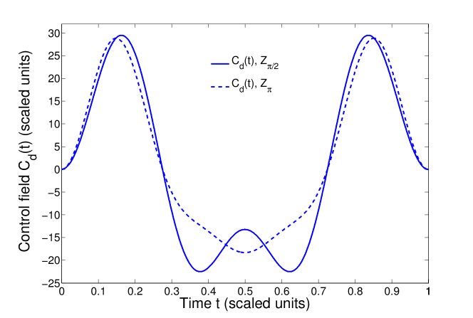
Figure 5: (Color online) Control fields satisfying the DPC in eq. (17), denoted as $C_{\mathrm{d}}(t)$, for $Z_{\phi}$ operations ($\vec{\eta}^{\,\mathrm{r}}\|_{2}<10^{-7}$), from Pasini et al. Pasini09a .

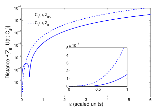
Figure 6: (Color online) Distance of the $Z_{\phi}$ operations as a function of $\varepsilon$ (with a resolution of 0.01 scaled units) and $\phi\in\{\pi/2,\pi\}$ for the Landau-Zener model of eq. (1) and control fields $C_{\mathrm{d}}(t)$ presented in fig. 5. The inset displays the gate distance for $0\leq\varepsilon\leq 1$ in greater detail, on a linear scale.

For a qubit described by the Hamiltonian in eq. (1), control fields from ref. Pasini09a satisfying $\|\vec{\eta}^{\,\mathrm{r}}\|_{2}<10^{-7}$ (where $\|\cdot\|_{2}$ denotes the vector two-norm) and corresponding gate-distances for $\pi/2$- and $\pi$-pulses are presented in figs. 5 and 6, respectively. These fields are denoted as $C_{\mathrm{d}}(t)$, where the subscript “d” indicates the decoupling feature of these DPs. Satisfying the control-field constraints specified by Pasini et al. Pasini09a , first- and second-order perturbations about $\varepsilon=0$ are eliminated. As such, gate distance increases with the magnitude of $\varepsilon$ and optimum performance occurs when $\varepsilon=0$, which is not necessarily expected to be valid for realistic qubit systems with drift terms, e.g., Petta05a . Although we use $\vec{\eta}^{\,\mathrm{r}}=0$ as a general condition for robustness in this work, whether controls satisfying $\vec{\eta}^{\,\mathrm{r}}=0$ are robust abouts points where $\varepsilon\neq 0$ remains an open question. However, comparing the gate distances in fig. 6 to figs. 3 and 4 reveals a certain degree of robustness in control fields $C_{\mathrm{d}}(t)$ relative to $C_{\mathrm{o}}(\varepsilon;t)$, e.g., for both $Z_{\phi}$ operations and all values of $\varepsilon_{0}$ considered, $\mathrm{d}\Delta/\mathrm{d}\varepsilon$ around $\varepsilon_{0}$ for $C_{\mathrm{d}}(t)$ is much smaller than $C_{\mathrm{o}}(\varepsilon_{0};t)$. Table 3 contains information about some of the properties of the DPs in figs. 5 and 6.

Target operation: $\bm{Z_{\pi/2}}$
$\varepsilon_{0}$	0	1	2	3	4	5
$\Delta(Z_{\pi/2},U_{t_{\mathrm{f}}})$	$7.60\times 10^{-8}$	$1.52\times 10^{-4}$	$1.34\times 10^{-3}$	$4.47\times 10^{-3}$	$1.02\times 10^{-2}$	$1.89\times 10^{-2}$
$\mathcal{R}_{\pi/2}[C_{\mathrm{d}},\varepsilon_{0},0.5]$	$2.84\times 10^{-6}$	$1.96\times 10^{-4}$	$1.42\times 10^{-3}$	$4.58\times 10^{-3}$	$1.03\times 10^{-2}$	$1.91\times 10^{-2}$

$\max|C_{\mathrm{d}}|=29.5$

$\theta(t_{\mathrm{f}};C_{\mathrm{d}})=\pi/2$

$\Phi[C_{\mathrm{d}}]=335.5$

$\|\vec{\eta}^{\,\mathrm{r}}(t;C_{\mathrm{d}})\|_{2}=2.52\times 10^{-8}$

Target operation: $\bm{Z_{\pi}}$
$\varepsilon_{0}$	0	1	2	3	4	5
$\Delta(Z_{\pi},U_{t_{\mathrm{f}}})$	$5.67\times 10^{-8}$	$5.84\times 10^{-4}$	$4.63\times 10^{-3}$	$1.54\times 10^{-2}$	$3.56\times 10^{-2}$	$6.75\times 10^{-2}$
$\mathcal{R}_{\pi}[C_{\mathrm{d}},\varepsilon_{0},0.5]$	$1.83\times 10^{-5}$	$7.29\times 10^{-4}$	$4.91\times 10^{-3}$	$1.58\times 10^{-2}$	$3.61\times 10^{-2}$	$6.81\times 10^{-2}$

$\max|C_{\mathrm{d}}|=28.8$

$\theta(t_{\mathrm{f}};C_{\mathrm{d}})=\pi$

$\Phi[C_{\mathrm{d}}]=264.8$

$\|\vec{\eta}^{\,\mathrm{r}}(t;C_{\mathrm{d}})\|_{2}=8.04\times 10^{-8}$

Table 3: Performance of the DPs $C_{\mathrm{d}}(t)$ for one-qubit $Z_{\phi}$ operations. Here, $\Delta$, $\mathcal{R}_{\phi}$, $\max|C_{\mathrm{d}}|$, $\theta$, $\Phi[C]:=\int_{0}^{t_{\mathrm{f}}}\!C^{2}(\varepsilon_{0};t)\mathrm{d}t$, and $\|\vec{\eta}^{\,\mathrm{r}}\|_{2}$ are the gate distance, gate robustness, maximum control-field amplitude, angle of controlled $z$-axis rotation, control-field fluence, and constraint vector norm, respectively, in the corresponding scaled units described in section II.3.

VI Hybrid quantum control: decoupling-pulse criteria + optimal control theory

Given the favorable structure of quantum-control landscapes, e.g., trap-free structure, continua corresponding to optimal solutions, etc., for regular controls Rabitz04a ; Ho09a ; Dominy11a ; Moore11b , DMORPH provides a mathematical means to explore families of controls that achieve the same objective Rothman05a ; Dominy08a . Applications of DMORPH include the continuous variation of a Hamiltonian while preserving or optimizing the value of a quantum-mechanical observable Rothman05a ; Donovan11a and exploring the level sets of state and unitary control Rothman06a ; Beltrani07a ; Dominy08a . DMORPH can also be used as direct optimization technique Moore11a . We develop DMORPH techniques to explore the space of controls corresponding to $\vec{\eta}=0$ while optimizing $\mathcal{J}$ for a specified $\varepsilon_{0}$.

Expressed more formally, in this section, we develop a method to optimize $\mathcal{J}$ over the set $\mathfrak{C}_{t_{\mathrm{f}}}^{\eta}:=\vec{\eta}^{\,-1}(0)\subset\mathfrak{C}_{t_{\mathrm{f}}}$, i.e., the set of feasible controls satisfying $\vec{\eta}=0$, where $\vec{\eta}^{-1}$ denotes the preimage of $\vec{\eta}$ . To increase general applicability, we develop this technique for $\vec{\eta}$, rather than the reduced constraint $\vec{\eta}^{\,\mathrm{r}}$. Away from critical points of $\vec{\eta}$ (a real-valued vector), i.e., controls for which the set of gradients $\{\nabla\eta_{i}\}$ are linearly dependent Guillemin74a , $\mathfrak{C}_{t_{\mathrm{f}}}^{\eta}$ is a codimension 5 submanifold of $\mathfrak{C}_{t_{\mathrm{f}}}$ Abraham88a . It is assumed that critical points of $\vec{\eta}$ are rare, an assumption supported by the success of the resulting algorithm. The gradient of the restricted functional $\mathcal{K}:=\mathcal{J}\big{|}_{\mathfrak{C}_{t_{\mathrm{f}}}^{\eta}}$ at a point $C\in\mathfrak{C}_{t_{\mathrm{f}}}^{\eta}$ is just the projection of the gradient of $\mathcal{J}$ at $C$ onto the tangent space $\mathrm{T}_{C}\mathfrak{C}_{t_{\mathrm{f}}}^{\eta}$ of $\mathfrak{C}_{t_{\mathrm{f}}}^{\eta}$ at $C$ doCarmo92a ; Milnor97a ; Dominy08a . By systematically updating the control field iteratively using a GrA with this projected gradient, the algorithm is able to simultaneously improve the value of $\mathcal{J}$ and maintain approximate feasibility, or at least impede deviations from feasibility. It is unlikely that the quantum-control landscape for the restricted objective functional $\mathcal{K}$ is trap-free. As such, a global optimization algorithm might be better suited to finding solutions. However, because a global parameterization of the set $\mathfrak{C}_{t_{\mathrm{f}}}^{\eta}$ is lacking, maintaining (approximate) feasibility, i.e., $\vec{\eta}=0$, might be difficult in general.

VI.1 Gradients of the feasibility constraints

Using DMORPH to remove the components of $\nabla\mathcal{J}$ that cause a change in $\vec{\eta}$ requires the gradient of each element of $\vec{\eta}$, $\nabla\eta_{i}$:

$$\left(\nabla\eta_{i}[C]\right)(t)=\int_{0}^{t_{\mathrm{f}}}\!\frac{\delta\zeta_{i}[\theta]}{\delta\theta(\tau)}\times\frac{\delta\theta(\tau)}{\delta C(t)}\mathrm{d}\tau=\int_{t}^{t_{\mathrm{f}}}\!\frac{\delta\zeta_{i}[\theta]}{\delta\theta(\tau)}\mathrm{d}\tau\ \Rightarrow$$ (19a)

$$\left(\begin{array}[]{c}\displaystyle{\left(\nabla\eta_{1}[C]\right)(t)}\\ \vdots\\ \displaystyle{\left(\nabla\eta_{5}[C]\right)(t)}\end{array}\right)=\left(\begin{array}[]{c}\displaystyle{\int_{t}^{t_{\mathrm{f}}}\!\cos[\theta(\tau)]\mathrm{d}\tau}\\ \displaystyle{\int_{t}^{t_{\mathrm{f}}}\!\sin[\theta(\tau)]\mathrm{d}\tau}\\ \displaystyle{2\int_{t}^{t_{\mathrm{f}}}\!\!\int_{0}^{t_{\mathrm{f}}}\!\!\big{\{}\cos[\theta(\tau)]\cos[\theta(\tau^{\prime})]+\sin[\theta(\tau)]\sin[\theta(\tau^{\prime})]\big{\}}\mathrm{sgn}(\tau-\tau^{\prime})\mathrm{d}\tau^{\prime}\mathrm{d}\tau}\\ \displaystyle{\int_{t}^{t_{\mathrm{f}}}\!\tau\cos[\theta(\tau)]\mathrm{d}\tau}\\ \displaystyle{\int_{t}^{t_{\mathrm{f}}}\!\tau\sin[\theta(\tau)]\mathrm{d}\tau}\end{array}\right).$$ (19j)

As expressed here, the vector of gradients $\nabla\eta_{i}$ is a function of the time variable $t$. Note that the set $\{\nabla\eta_{i}\}$ spans the normal space $\left(\mathrm{T}_{C}\mathfrak{C}_{t_{\mathrm{f}}}^{\eta}\right)^{\perp}$ when $C\in\mathfrak{C}_{t_{\mathrm{f}}}^{\eta}$ is a regular point of $\vec{\eta}$.

VI.2 Gradient projection method

In addition to the gradients $\nabla\eta_{i}$, we also need a vector that specifies the relative weight of each gradient component to remove. This is determined by first calculating the Gramian matrix, with elements

$$\left(G_{c}\right)_{ij}:=\left\langle\nabla\eta_{i}[C],\nabla\eta_{j}[C]\right\rangle_{\mathfrak{C}_{t_{\mathrm{f}}}}.$$ (20)

In general, $G_{c}$ is not guaranteed to be full rank; non-singularity of $G_{c}$ must be explored (numerically) as a function of $C$. The Gramian matrix $G_{c}$ is rank deficient if and only if elements in the set $\{\nabla\eta_{i}\}$ are linearly dependent, i.e., if and only if $C$ is a critical point of $\vec{\eta}$ Guillemin74a . However, when $\nabla\eta_{i}$ are all linearly independent, $G_{c}$ is invertible. With eqs. (19) and (20), all gradient directions $\nabla\eta_{i}$ can be removed from $\nabla\mathcal{J}$, producing $\nabla\mathcal{K}$ as follows:

$$\nabla\mathcal{K}[C]=\nabla\mathcal{J}[C]-\sum_{i=1}^{5}\nabla\eta_{i}[C]\left\{G_{c}^{-1}\left[\vec{q}_{c}\left(\nabla\mathcal{J}[C]\right)\right]\right\}_{i},$$ (21a)

where $$\mathcal{K}:\mathfrak{C}_{t_{\mathrm{f}}}^{\eta}\to\mathbb{R} \mathcal{J} \mathcal{K}:=\mathcal{J}|_{\mathfrak{C}_{t_{\mathrm{f}}}^{\eta}} \vec{q}_{c}$$ is a restriction of , i.e., , and has elements

$$\left[\vec{q}_{c}\left(\nabla\mathcal{J}[C]\right)\right]_{i}:=\left\langle\nabla\mathcal{J}[C],\nabla\eta_{i}[C]\right\rangle_{\mathfrak{C}_{t_{\mathrm{f}}}}.$$ (21b)

Thus, $\nabla\mathcal{K}$ is a vector field on $\mathfrak{C}_{t_{\mathrm{f}}}^{\eta}$, and the ordinary differential equation (ODE)

$$\frac{\mathrm{d}C(s)}{\mathrm{d}s}=-\nabla\mathcal{K}[C(s)]$$ (22)

describes the gradient flow of $\mathcal{K}$ on $\mathfrak{C}_{t_{\mathrm{f}}}^{\eta}$ that minimizes $\mathcal{J}$ without changing the value of $\vec{\eta}$. The GrA in this work implements a forward Euler integration of this equation, which should be sufficiently accurate, provided that the multiplier $\beta$ in eq. (11) is selected properly, i.e., $\beta$ is within the validity of the linear approximation of the tangent space at $C$. Higher-order numerical ODE solvers, e.g., Runge-Kutta methods Press92a , might offer higher accuracy and/or greater efficiency, but have not been explored in this work.

Equation (21) describes the orthogonal projection from $\mathrm{T}_{C}\mathfrak{C}_{t_{\mathrm{f}}}$ to $\mathrm{T}_{C}\mathfrak{C}_{t_{\mathrm{f}}}^{\eta}$. That $\nabla\mathcal{K}$ is orthogonal to all elements of $\{\nabla\eta_{i}\}$ can be verified as follows. Let

$$\xi:=\sum_{i=1}^{5}\chi_{i}\nabla\eta_{i}[C],$$ (23)

i.e., $\xi$ is a linear combination of the elements of the set $\left\{\nabla\eta_{i}\right\}$, where $\chi_{i}\in\mathbb{R}$. Replacing $\nabla\mathcal{J}$ with $\xi$ in eq. (21) yields

$$\xi-\sum_{i=1}^{5}\nabla\eta_{i}[C]\left\{G_{c}^{-1}\left[\vec{q}_{c}\left(\xi\right)\right]\right\}_{i}=\xi-\sum_{i=1}^{5}\nabla\eta_{i}[C]\left(G_{c}^{-1}G_{c}\vec{\chi}\right)_{i}=0,$$ (24)

where $\vec{\chi}:=(\chi_{1},\chi_{2},\chi_{3},\chi_{4},\chi_{5})^{\mathrm{T}}$. If $\xi\in\mathrm{T}_{C}\mathfrak{C}_{t_{\mathrm{f}}}$ is such that $\xi$ is orthogonal to all gradients $\nabla\eta_{i}$, then the projection described in eq. (21) acts as identity on $\xi$. Together with the previous statement, this shows that eq. (21) is the orthogonal projector from $\mathrm{T}_{C}\mathfrak{C}_{t_{\mathrm{f}}}$ to $\mathrm{T}_{C}\mathfrak{C}_{t_{\mathrm{f}}}^{\eta}$.

As mentioned in the introduction, because we combine DPC and OCT methods to generate improved control fields, we denote the integrated optimization procedure described in this section as DPC+OCT. Straightforward modifications of $G_{c}$ and $\vec{q}_{c}$ are required when $\vec{\eta}^{\,\mathrm{r}}$ is the constraint vector rather than $\vec{\eta}$, i.e., $G_{c}\in\mathcal{M}_{3}(\mathbb{R})$, rather than $\mathcal{M}_{5}(\mathbb{R})$, and $\vec{q}_{c}\left(\nabla\mathcal{J}\right)\in\mathbb{R}^{3}$, rather than $\mathbb{R}^{5}$.

VII Results from decoupling-pulse criteria + optimal control theory

Using the DPC+OCT protocol described in section VI and the DPs in fig. 5 for the initial iterations of all values of $\varepsilon_{0}$ considered, we sought to numerically explore the space of controls satisfying $\vec{\eta}^{\,\mathrm{r}}=0$ and $\Delta=0$ to improve control fidelity and robustness to $\varepsilon$-uncertainty for $Z_{\pi/2}$ and $Z_{\pi}$ operations, compared to the original DPs. To a certain extent, it appears a priori that the minimization of $\Delta$ and $\vec{\eta}^{\,\mathrm{r}}$ might be competing control objectives. For example, compare the gate-distance plots for OCT (figs. 3 and 4) to those for the DPs (fig. 6) over the interval $0\leq\varepsilon\leq 6$ (with a numerical resolution of 0.01 scaled units). OCT for the design of unitary operations, as we have formulated it in section III, seeks to minimize $\Delta$ for a particular value of $\varepsilon$, namely, the parameter estimate $\varepsilon_{0}$. Because the system described by the Hamiltonian in eq. (1) is controllable and the underlying control landscape possesses a fortuitous structure for regular controls Ho09a ; Dominy11a , a GrA achieves this objective quite efficiently and successfully. However, as presented in section IV, these OCs are not inherently robust to perturbations in $\varepsilon$, whereas controls satisfying $\vec{\eta}^{\,\mathrm{r}}=0$ are nearly optimal (with respect to $\mathcal{J}$) when $\varepsilon_{0}\approx 0$. This scenario illustrates the potential balance that can exist between fidelity and robustness in general. Overall, the controls that satisfy $\vec{\eta}^{\,\mathrm{r}}=0$ are reasonably robust to perturbations in $\varepsilon$, provided that $\varepsilon$ and/or $\Delta\varepsilon$ are within the perturbative limit. Given that these two control objectives are potentially competing, we use the hybrid optimization procedure developed in section VI to suppress deviations from $\vec{\eta}^{\,\mathrm{r}}=0$, but not entirely eliminate them. In other words, convergence of the DMORPH DPC+OCT algorithm occurs only when $\mathcal{J}$ stops decreasing, not when $\vec{\eta}^{\,\mathrm{r}}$ starts increasing.

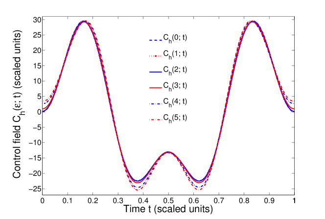
Figure 7: (Color online) DPC+OCT fields $C_{\mathrm{h}}(\varepsilon_{0};t)$ producing a $Z_{\pi/2}$ operation, optimized using $C_{\mathrm{d}}(t)$ as the initial control for all estimates/values of $\varepsilon_{0}$ and $t_{\mathrm{f}}=1$ scaled unit. Although distinct, note that $C_{\mathrm{h}}(0;t)$, $C_{\mathrm{h}}(1;t)$, and $C_{\mathrm{h}}(2;t)$ appear nearly indistinguishable in this figure.

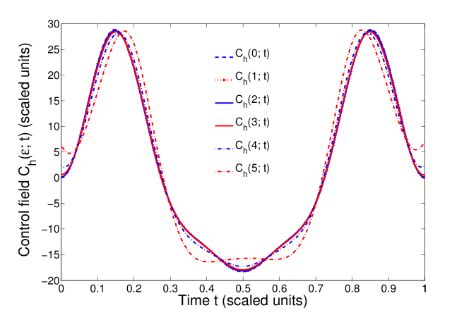
Figure 8: (Color online) DPC+OCT fields $C_{\mathrm{h}}(\varepsilon_{0};t)$ producing a $Z_{\pi}$ operation, optimized using $C_{\mathrm{d}}(t)$ as the initial control for all estimates/values of $\varepsilon_{0}$ and $t_{\mathrm{f}}=1$ scaled unit. Although distinct, note that $C_{\mathrm{h}}(0;t)$, $C_{\mathrm{h}}(1;t)$, and $C_{\mathrm{h}}(2;t)$ appear nearly indistinguishable in this figure.

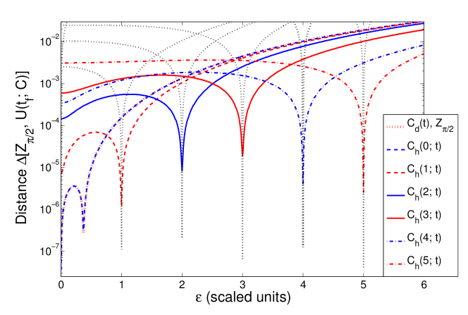
Figure 9: (Color online) Distance for the $Z_{\pi/2}$ operation as a function of $\varepsilon$ (with a resolution of 0.01 scaled units) for control fields satisfying (a) $\vec{\eta}^{\,\mathrm{r}}=0$ [red dashed line, which is very similar to that for $C_{\mathrm{h}}(0;t)$], (b) $\vec{\eta}^{\,\mathrm{r}}\approx 0$ and $\Delta\approx 0$, optimized with a specified value of $\varepsilon_{0}$, and (c) results from $C_{\mathrm{o}}(\varepsilon_{0};t)$ in section IV (black dashed lines, from fig. 3).

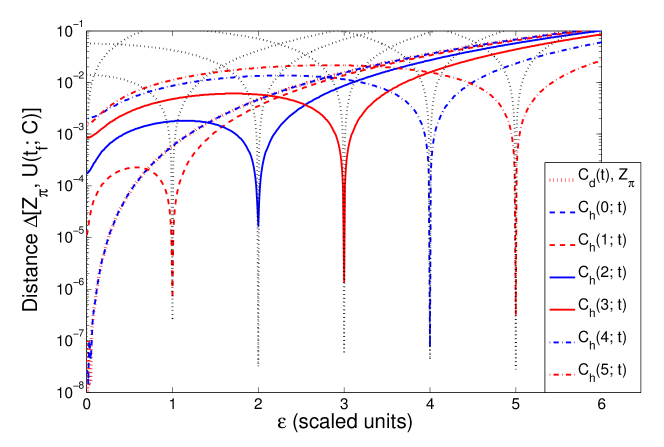
Figure 10: (Color online) Distance for the $Z_{\pi}$ operation as a function of $\varepsilon$ (with a resolution of 0.01 scaled units) for control fields satisfying (a) $\vec{\eta}^{\,\mathrm{r}}=0$ [red dashed line, which is very similar to that for $C_{\mathrm{h}}(0;t)$)], (b) $\vec{\eta}^{\,\mathrm{r}}\approx 0$ and $\Delta\approx 0$, optimized with a specified value of $\varepsilon_{0}$, and (c) results from $C_{\mathrm{o}}(\varepsilon_{0};t)$ in section IV (black dashed lines, from fig. 4).

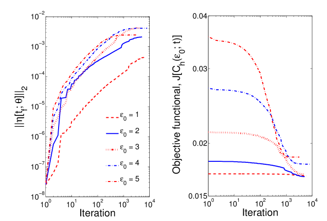
Figure 11: (Color online) $\|\vec{\eta}^{\,\mathrm{r}}\|_{2}$ and objective functional $\mathcal{J}$ for the $Z_{\pi/2}$ operation and each value of $\varepsilon_{0}$ considered, as a function of the number of DPC+OCT algorithm iterations.

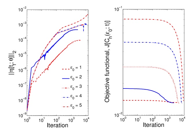
Figure 12: (Color online) $\|\vec{\eta}^{\,\mathrm{r}}\|_{2}$ and objective functional $\mathcal{J}$ for the $Z_{\pi}$ operation and each value of $\varepsilon_{0}$ considered, as a function of the number of DPC+OCT algorithm iterations.

Because the formulation of OCT requires the specification of $\varepsilon$, we consider $\varepsilon_{0}\in[0,5]$. As before, the final time for all controls was fixed at $t_{\mathrm{f}}=1$ scaled unit of time. DPC+OCT fields for $Z_{\pi/2}$ and $Z_{\pi}$ are presented in fig. 7 and fig. 8, respectively. These fields are denoted as $C_{\mathrm{h}}(\varepsilon_{0};t)$, where the subscript “h” indicates the hybrid feature of this QCP. Corresponding results for the gate distance $\Delta$ are presented in figs. 9 and 10; results for the vector-constraint norm $\|\vec{\eta}^{\,\mathrm{r}}\|_{2}$, and objective functional $\mathcal{J}$ are presented in figs. 11 and 12. In addition, table 4 contains information about some of the properties of the DPC+OCT fields. For both $Z_{\phi}$ operations, when $\varepsilon_{0}\geq 2$, we note that $\|\vec{\eta}^{\,\mathrm{r}}\|_{2}>10^{-4}$. However, since the robustness criteria quantified by $\vec{\eta}^{\,\mathrm{r}}$ were obtained from a perturbative analysis about $\varepsilon_{0}=0$, it remains an open question whether, a priori, control fields satisfying $\vec{\eta}^{\,\mathrm{r}}=0$ for $\varepsilon_{0}>0$ will be robust to fluctuations about $\varepsilon_{0}$. However, as we present in this section, control solutions obtained from the DPC+OCT protocol have some desireable properties, even when $\varepsilon_{0}>0$. It is interesting to explore the results of the DPC+OCT protocol when the distance is relatively large (i.e., $\Delta>10^{-3}$) and the sensitivity to changes in $\varepsilon$ is small, e.g., as illustrated in fig. 6.

Despite their unique gate-distance dependence of these control solutions on $\varepsilon$, as shown in figs. 9 and 10 over the interval $0\leq\varepsilon\leq 6$ (with a numerical resolution of 0.01 scaled units), the converged DPC+OCT fields for $\varepsilon_{0}\in\{0,1,2,3\}$ are very similar to each other and the originated DP for each target unitary operation. This supports the observation in section IV that this simple system can effectively discriminate between very similar control fields, i.e., as measured by the gate distance $\Delta$ in eq. (4), the qubit system is quite sensitive to these relatively small control-field variations. For example, although $\max_{t}\left|C_{\mathrm{h}}(1;t)-C_{\mathrm{h}}(2;t)\right|<0.2$ scaled units of energy for both operations, and the mean relative difference is approximately 1.5% and 1.3% for the $Z_{\pi/2}$ and $Z_{\pi}$ operations, respectively, the corresponding gate distances (presented in figs. 9 and 10) do not coincide significantly when $0\leq\varepsilon\leq 3$.

Interestingly, the DPC+OCT control field for the $Z_{\pi}$ operation when $\varepsilon_{0}=5$ has some distinguishing features compared to the fields for the other values of $\varepsilon_{0}$. Based on the relatively large distance $\Delta$ of the corresponding $C_{\mathrm{d}}(t)$ control used for the initial iterate in the DPC+OCT protocol ($\Delta=6.75\times 10^{-2}$), this value of $\varepsilon_{0}$ is not within the perturbative limit of the analysis that produced the vector constraint $\vec{\eta}^{\,\mathrm{r}}=0$. With such a large distance at $\varepsilon_{0}=5$, the DPC+OCT routine improves the distance by a factor larger than $10^{4}$ and simultaneously improves the robustness $\mathcal{R}_{\pi}$ for $4.5\leq\varepsilon\leq 5.5$ by a factor larger than 10, compared to the corresponding results for $C_{\mathrm{d}}(t)$ presented in table 3.

Figures 9 and 10 compare the distance of $C_{\mathrm{d}}(t)$ and $C_{\mathrm{h}}(\varepsilon_{0};t)$ control fields for both $Z_{\phi}$ operations. Compared to $C_{\mathrm{d}}(t)$, all control fields $C_{\mathrm{h}}(\varepsilon_{0};t)$ for $\varepsilon_{0}\geq 0$ exhibit improved robustness to $\varepsilon$-uncertainties in an interval around the nominal value $\varepsilon_{0}$ used in the DPC+OCT algorithm. This result demonstrates the utility of combining so-called “pre-design” methods, which are based on mathematically analyzing general models [e.g., eq. (14)], such as the DPC developed by Pasini et al. Pasini09a , with numerical OCT procedures and simple estimates of system parameters (e.g., estimates of $\varepsilon_{0}$), especially when capabilities for shaping control fields are available. By combining these QCPs, we have developed a form of hybrid quantum control; estimates of system parameters can be directly incorporated into simulations to generate improved quantum operations for information processing and memory.

Figures 11 and 12 compare the vector-constraint norm $\|\vec{\eta}^{\,\mathrm{r}}\|_{2}$ and objective functional $\mathcal{J}$ as a function of the optimization iteration for both $Z_{\phi}$ operations. Overall, $\|\vec{\eta}^{\,\mathrm{r}}\|_{2}$ increases as $\mathcal{J}$ decreases, which is consistent with the notion of minimizing $\|\vec{\eta}^{\,\mathrm{r}}\|_{2}$ and $\mathcal{J}$ as potentially competing control objectives. Even though components of $\nabla\mathcal{J}$ that are parallel to all gradients $\nabla\eta_{i}$ are removed at each iteration, $\|\vec{\eta}^{\,\mathrm{r}}\|_{2}$ increases during the optimization for (at least) two reasons: (a) eq. (21) removes components of $\nabla\eta_{i}$ (where elements $\eta_{i}$ are nonlinear functions of the control) using an iterative linear projection method and (b) convergence of the DPC+OCT routine does not depend on $\|\vec{\eta}^{\,\mathrm{r}}\|_{2}$.

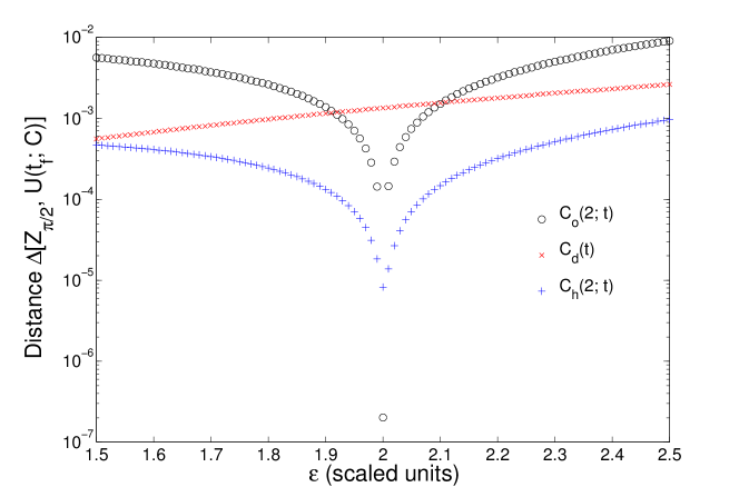
Figure 13: (Color online) Distance for the $Z_{\pi/2}$ operation as a function of $\varepsilon$ for $C_{\mathrm{o}}(2;t)$, $C_{\mathrm{d}}(t)$, and $C_{\mathrm{h}}(2;t)$ controls in a unit interval centered at $\varepsilon_{0}=2$ (with a resolution of 0.01 scaled units). Note that for $\varepsilon\geq 0.7$, $\Delta[Z_{\pi},U(t_{\mathrm{f}};C_{\mathrm{d}})]\geq\Delta[Z_{\pi},U(t_{\mathrm{f}};C_{\mathrm{h}})]$, i.e., $C_{\mathrm{h}}(1;t)$ outperforms $C_{\mathrm{d}}(t)$.

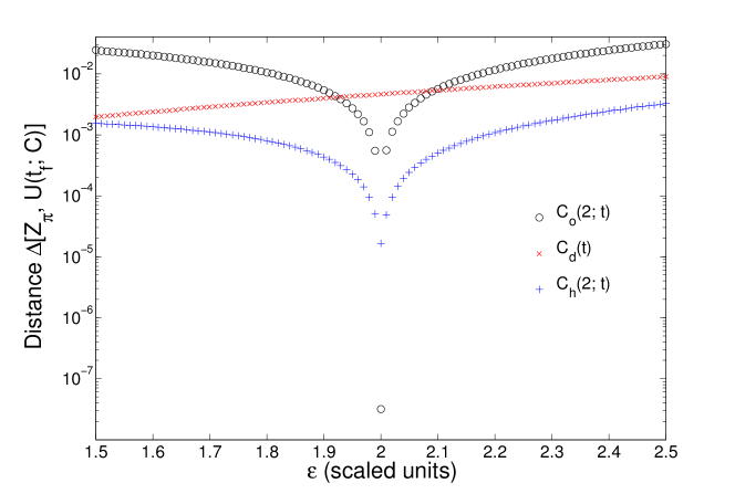
Figure 14: (Color online) Distance for the $Z_{\pi}$ operation as a function of $\varepsilon$ for $C_{\mathrm{o}}(2;t)$, $C_{\mathrm{d}}(t)$, and $C_{\mathrm{h}}(2;t)$ controls in a unit interval centered at $\varepsilon_{0}=2$ (with a resolution of 0.01 scaled units). Note that for $\varepsilon\geq 1.5$, $\Delta[Z_{\pi},U(t_{\mathrm{f}};C_{\mathrm{d}})]\geq\Delta[Z_{\pi},U(t_{\mathrm{f}};C_{\mathrm{h}})]$, i.e., $C_{\mathrm{h}}(1;t)$ outperforms $C_{\mathrm{d}}(t)$.

To aid in the comparative analysis of results from OCT, DPC, and the DPC+OCT procedures, OC gate-distance data from figs. 3 and 4 are also presented in figs. 9 and 10, respectively. Although the OC fields $C_{\mathrm{o}}(\varepsilon_{0};t)$ all outperform the DPC+OCT fields $C_{\mathrm{h}}(\varepsilon_{0};t)$ at $\varepsilon_{0}$, these OCs do not have the robustness of the DPs or DPC+OCT fields. To emphasize this feature, figs. 13 and 14 present $Z_{\pi/2}$ and $Z_{\pi}$ gate distances for $C_{\mathrm{o}}(2;t)$, $C_{\mathrm{d}}(t)$, and $C_{\mathrm{h}}(2;t)$ controls over a unit interval centered at $\varepsilon_{0}=2$. For both gates, $C_{\mathrm{o}}(2;t)$ is very sensitive to variations in $\varepsilon$, e.g., when $\varepsilon$ changes from 2 to $2\pm 0.01$ (a change corresponding to approximately $1.3\times 10^{-5}$ T for the GaAs DQD example), the $Z_{\pi/2}$ gate distance increases (approximately) from $10^{-7}$ to $10^{-4}$, while the $Z_{\pi}$ gate distance increases from $10^{-8}$ to $10^{-4}$, approaching the fault-tolerant threshold. However, for $C_{\mathrm{h}}(2;t)$ for both gates, as $\varepsilon$ varies from $\varepsilon_{0}$, the increase in gate distance is much more gradual. Figures 13 and 14 contain some useful information to help understand the benefit of the hybrid DPC+OCT protocol. By combining DPC, OCT, a DP that satisfies $\vec{\eta}^{\,\mathrm{r}}=0$ for the initial GrA iteration, and an estimate of the value of $\varepsilon_{0}$, the gate distance is decreased compared to the gate distance of the original DP for the entire unit interval centered at $\varepsilon_{0}$. Depending on the uncertainty magnitude of $\varepsilon$, this benefit could yield a potentially substantial decrease in the required concatenation/encoding resources necessary for QECCs, which depend on gate errors.

As a final illustrative example, consider the $Z_{\pi}$ operation applied to the initial state $|\sigma_{x}^{+}\rangle$, implemented with the corresponding controls $C_{\mathrm{o}}(2;t)$, $C_{\mathrm{d}}(t)$, and $C_{\mathrm{h}}(2;t)$, which are applied to an ensemble of systems described by the Hamiltonian in eq. (1) and the interval $1.5\leq\varepsilon\leq 2.5$ (numerically distributed over 20 equal increments of 0.05 scaled units). The target state is $|\sigma_{x}^{-}\rangle=Z_{\pi}|\sigma_{x}^{+}\rangle$, where $\sigma_{x}|\sigma_{x}^{\pm}\rangle=\pm|\sigma_{x}^{\pm}\rangle$, and the ensemble of final states for a given control is denoted by $\{|\psi_{i}\rangle\}$. This state-based example clarifies the gate improvement obtained from $C_{\mathrm{h}}(2;t)$, compared to $C_{\mathrm{o}}(2;t)$ and $C_{\mathrm{d}}(t)$. To quantify the fidelity of the controls, we use the Uhlmann state fidelity for pure states Uhlmann76a ; Jozsa94a :

$$\mathcal{F}_{\mathrm{u}}\left(|\psi_{1}\rangle,|\psi_{2}\rangle\right):=\left|\langle\psi_{1}|\psi_{2}\rangle\right|,$$ (25)

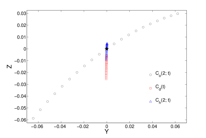
Figure 15: (Color online) Final state in the Bloch vector coordinates $y$ and $z$ for the $Z_{\pi}$ operation, implemented with the corresponding controls $C_{\mathrm{o}}(2;t)$, $C_{\mathrm{d}}(t)$, and $C_{\mathrm{h}}(2;t)$ applied to an ensemble of systems described by the Hamiltonian in eq. (1) and the interval $1.5\leq\varepsilon\leq 2.5$ (distributed over 20 equal increments of 0.05 scaled units). The target state is $|\sigma_{x}^{-}\rangle=Z_{\pi}|\sigma_{x}^{+}\rangle$. Because $-1\leq x<-0.995$ for all final states, it is not included in this figure.

where $|\psi_{1}\rangle$ and $|\psi_{2}\rangle$ are normalized vectors in $\mathcal{H}$. For a given control, we denote the resulting minimum, maximum, and average state fidelity, and the standard deviation of the fidelity of the ensemble as $\min_{|\psi_{i}\rangle}\mathcal{F}_{\mathrm{u}}$, $\max_{|\psi_{i}\rangle}\mathcal{F}_{\mathrm{u}}$, $\bar{\mathcal{F}}_{\mathrm{u}}$, and $\sigma_{\mathcal{F}_{\mathrm{u}}}$, respectively, which are presented in table 5 for $C_{\mathrm{o}}(2;t)$, $C_{\mathrm{d}}(t)$, and $C_{\mathrm{h}}(2;t)$. Comparing the respective quantities, $C_{\mathrm{h}}(2;t)$ has the largest average and minimum fidelity and the smallest standard deviation of fidelity of the ensemble (by nearly a factor of 10). The final-time ensembles are also illustrated in fig. 15, which contains a plot of resulting final states for each control, along with the target state $|\sigma_{x}^{-}\rangle$, all in the Bloch vector coordinates $y$ and $z$. Because $-1\leq x<-0.995$ for all final states, it is not included in this figure. Unlike the Bloch vector components corresponding to the final states produced from $C_{\mathrm{o}}(2;t)$ and $C_{\mathrm{d}}(t)$, the Bloch vector components produced from $C_{\mathrm{h}}(2;t)$ are tightly distributed around the target state, with most of the error distributed uniformly along the $z$-axis, centered at the target state $|\sigma_{x}^{-}\rangle$. Very similar results are obtained for the $Z_{\pi/2}$ operation implemented with $C_{\mathrm{o}}(2;t)$, $C_{\mathrm{d}}(t)$, and $C_{\mathrm{h}}(2;t)$, applied to an ensemble of systems where $1.5\leq\varepsilon\leq 2.5$.

Target operation: $\bm{Z_{\pi/2}}$
$\varepsilon_{0}$	0	1	2	3	4	5
$\max|C_{\mathrm{h}}|$	29.5	29.5	29.3	29.2	29.4	29.6
$\theta(t_{\mathrm{f}};C_{\mathrm{h}})$	$\pi/2$	$\pi/2$	1.5704	1.5690	1.5695	1.5792
$\Phi[C_{\mathrm{h}}]$	335.5	334.6	332.8	337.4	356.5	370.5
$\Delta(Z_{\pi/2},U_{t_{\mathrm{f}}})$	$3.65\times 10^{-8}$	$1.21\times 10^{-6}$	$8.23\times 10^{-6}$	$1.86\times 10^{-5}$	$4.08\times 10^{-6}$	$2.55\times 10^{-6}$
$\|\vec{\eta}^{\,\mathrm{r}}(t_{\mathrm{f}};C_{\mathrm{h}})\|_{2}$	$3.21\times 10^{-8}$	$4.74\times 10^{-4}$	$2.13\times 10^{-3}$	$4.21\times 10^{-3}$	$4.12\times 10^{-3}$	$2.45\times 10^{-3}$
$\mathcal{R}_{\pi/2}[C_{\mathrm{h}},\varepsilon_{0},0.5]$	$2.84\times 10^{-6}$	$9.47\times 10^{-5}$	$3.55\times 10^{-4}$	$6.46\times 10^{-4}$	$5.72\times 10^{-4}$	$9.20\times 10^{-4}$
Target operation: $\bm{Z_{\pi}}$
$\varepsilon_{0}$	0	1	2	3	4	5
$\max|C_{\mathrm{h}}|$	28.8	28.8	28.6	28.4	28.4	28.9
$\theta(t_{\mathrm{f}};C_{\mathrm{h}})$	$\pi$	$\pi$	3.1411	3.1392	3.1343	3.1320
$\Phi[C_{\mathrm{h}}]$	264.8	264.0	261.8	259.1	260.0	280.7
$\Delta(Z_{\pi},U_{t_{\mathrm{f}}})$	$2.36\times 10^{-8}$	$6.57\times 10^{-7}$	$1.67\times 10^{-5}$	$1.74\times 10^{-5}$	$2.79\times 10^{-8}$	$1.10\times 10^{-6}$
$\|\vec{\eta}^{\,\mathrm{r}}(t_{\mathrm{f}};C_{\mathrm{h}})\|_{2}$	$3.55\times 10^{-9}$	$9.93\times 10^{-5}$	$4.90\times 10^{-4}$	$1.10\times 10^{-3}$	$6.49\times 10^{-3}$	$2.10\times 10^{-2}$
$\mathcal{R}_{\phi}[C_{\mathrm{h}},\varepsilon_{0},0.5]$	$1.83\times 10^{-5}$	$3.11\times 10^{-4}$	$1.18\times 10^{-3}$	$2.59\times 10^{-3}$	$4.23\times 10^{-3}$	$4.92\times 10^{-3}$

Table 4: Performance of the DPC+OCT controls $C_{\mathrm{h}}(\epsilon_{0};t)$ for one-qubit $Z_{\phi}$ operations. Here, $\max|C_{\mathrm{h}}|$, $\theta$, $\Phi[C]:=\int_{0}^{t_{\mathrm{f}}}\!C^{2}(\varepsilon_{0};t)\mathrm{d}t$, $\Delta$, $\|\vec{\eta}^{\,\mathrm{r}}\|_{2}$, and $\mathcal{R}_{\phi}$ are the maximum control-field amplitude, angle of controlled $z$-axis rotation, control-field fluence, gate distance, constraint vector norm, and gate robustness, respectively, in the corresponding scaled units described in section II.3.

Target state: $\bm{|\sigma_{x}^{-}\rangle=Z_{\pi}|\sigma_{x}^{+}\rangle}$
	$\displaystyle{\min_{|\psi_{i}\rangle}\mathcal{F}_{\mathrm{u}}\left[|\sigma_{x}^{-}\rangle,|\psi_{i}\rangle\right]}$	$\displaystyle{\max_{|\psi_{i}\rangle}\mathcal{F}_{\mathrm{u}}\left[|\sigma_{x}^{-}\rangle,|\psi_{i}\rangle\right]}$	$\bar{\mathcal{F}}_{\mathrm{u}}$	$\sigma_{\mathcal{F}_{\mathrm{u}}}$
$C_{\mathrm{o}}(2;t)$	0.996197	1.0	0.998871	$1.082\times 10^{-3}$
$C_{\mathrm{d}}(t)$	0.999678	0.999985	0.999884	$9.398\times 10^{-5}$
$C_{\mathrm{h}}(2;t)$	0.999958	1.0	0.999991	$1.129\times 10^{-5}$

Table 5: Properties of state fidelity for the transition $|\sigma_{x}^{-}\rangle=Z_{\pi}|\sigma_{x}^{+}\rangle$ driven by controls $C_{\mathrm{o}}(2;t)$, $C_{\mathrm{d}}(t)$, and $C_{\mathrm{h}}(2;t)$. Here, $\min_{|\psi_{i}\rangle}\mathcal{F}_{\mathrm{u}}$, $\max_{|\psi_{i}\rangle}\mathcal{F}_{\mathrm{u}}$, $\bar{\mathcal{F}}_{\mathrm{u}}$, and $\sigma_{\mathcal{F}_{\mathrm{u}}}$ denote the minimum, maximum, and average fidelity, and the standard deviation of the fidelity, respectively, of the ensemble of final states $\{|\psi_{i}\rangle\}$ compared to the target state $|\sigma_{x}^{-}\rangle$.

VIII Conclusions and future directions

Combining OCT with the DPC established by Pasini et al. introduces improvements to the control of quantum systems for information processing. Given a reasonable characterization of the angular frequency $\varepsilon/\hbar$ of a persistent, but somewhat uncertain rotation about the $x$-axis, a near-optimal fidelity can be achieved for $\varepsilon\geq 0$. Furthermore, the resulting DPC+OCT controls exhibit improved robustness to uncertainty in $\varepsilon$, compared to the original DPs. The systematic integration of general DPC and control-field shaping methods from OCT, therefore, promises considerable improvement over DPC or OCT strategies alone. We have provided a quantitative illustration for a logical qubit based on a DQD system, with continuous controls that possess reasonable magnitudes Nielsen10a , based on the scaled-to-SI unit mapping.

We are currently investigating the benefits of these DPC+OCT $\pi/2$- and $\pi$-pulses for memory and information processing in the presence of a decohering spin bath. It will be useful to determine how these pulses extend spin-echoes and improve general DD and dynamically-corrected gate pulse sequences, such as those described in refs. Liu07a ; Uhrig08a ; Khodjasteh05a ; Khodjasteh07a ; Khodjasteh09a ; Khodjasteh09b ; Khodjasteh10a ; Pasini11a . Future work involves an exploration of unitary control sensitivity to fluctuations in the control field itself (e.g., control noise). Post facto analysis of both the OCT and DPC+OCT results presented in this article for the general qubit model suggests that these fluctuations may contribute just as significantly to gate errors as corresponding system and environment fluctuations. However, our optimization criteria does not include robustness to control-field noise; such robustness may be sacrificed in favor of the actual criteria. Given the ubiquity of noise in classical controls and quantum-mechanical systems, constructing controls and systems that are robust to their own noise is crucial for practical fault-tolerant QC.

Extensions of the original analysis by Pasini et al. are also being considered. We are interested in generalizing their results to include (a) arbitrary angle rotations and axes, (b) closed-system perturbative expansions about any value of $\varepsilon$, rather than only $\varepsilon=0$, and (c) $\varepsilon$ as a stochastic time-dependent variable/operator, which is relevant to previous research on decoherence control, e.g., Young10a . In addition, direct minimization of $\mathcal{R}_{\phi}$ [eq. (13)] or

$$\mathcal{L}[C]:=\int_{\varepsilon_{1}}^{\varepsilon_{2}}\!\left(c_{1}\left\|\frac{\mathrm{d}U_{t_{\mathrm{f}}}(C)}{\mathrm{d}\varepsilon}\right\|_{\mathrm{HS}}+c_{2}\left\|\frac{\mathrm{d}^{2}U_{t_{\mathrm{f}}}(C)}{\mathrm{d}\varepsilon^{2}}\right\|_{\mathrm{HS}}\right)\mathrm{d}\varepsilon$$ (26)

over $\mathcal{J}^{-1}(0)$, where $c_{1}$, $c_{2}\in\mathbb{R}$ weight the relative significance of the two norms, are purely OCT means to improve robustness to variations in $\varepsilon$ about any fixed interval $\left[\varepsilon_{1},\varepsilon_{2}\right]$, which we are also investigating.

Figures

References

- (1) F. Gaitan, Quantum Error Correction and Fault Tolerant Quantum Computing (CRC Press, Boca Raton, FL, 2008)
- (2) T. D. Ladd, F. Jelezko, R. Laflamme, Y. Nakamura, C. Monroe, and J. L. O’Brien, Nature 464, 45 (Mar 2010)
- (3) R. Liu, W. Yao, and L. J. Sham, New J. Phys. 9, 226 (2007)
- (4) G. S. Uhrig, New J. Phys. 10, 083024 (2008)
- (5) R. Roloff, M. Wenin, and W. Pötz, J. Comp. Theor. Nano. 6, 1837 (Aug 2009)
- (6) C. Brif, R. Chakrabarti, and H. Rabitz, New J. Phys. 12, 075008 (Jul 2010)
- (7) D. A. Lidar and K. B. Whaley, in Irreversible Quantum Dynamics, Lecture Notes in Physics, Vol. 622, edited by F. Benatti and R. Floreanini (Springer-Verlag, Berlin, 2003) Chap. 3, pp. 83–120
- (8) P. Zanardi and M. Rasetti, Phys. Rev. Lett. 79, 3306 (Oct 1997)
- (9) C. Nayak, S. H. Simon, A. Stern, M. Freedman, and S. Das Sarma, Rev. Mod. Phys. 80, 1083 (2008)
- (10) J. Werschnik and E. K. U. Gross, J. Phys. B: At. Mol. Opt. Phys. 40, R175 (2007)
- (11) G. S. Uhrig, Phys. Rev. Lett. 98, 100504 (Mar 2007)
- (12) P. Karbach, S. Pasini, and G. S. Uhrig, Phys. Rev. A 78, 022315 (2008)
- (13) S. Pasini, T. Fischer, P. Karbach, and G. S. Uhrig, Phys. Rev. A 77, 032315 (Mar 2008)
- (14) S. Pasini and G. S. Uhrig, J. Phys. A: Math. and Theor. 41, 312005 (2008)
- (15) S. Pasini, P. Karbach, C. Raas, and G. S. Uhrig, Phys. Rev. A 80, 022328 (Aug 2009)
- (16) S. Pasini and G. S. Uhrig, J. Phys. A: Math. and Theor. 43, 132001 (2010)
- (17) S. Pasini, P. Karbach, and G. S. Uhrig, Europhys. Lett. 96, 10003 (Oct 2011)
- (18) J. P. Palao and R. Kosloff, Phys. Rev. A 68, 062308 (Dec 2003)
- (19) A. Messiah, Quantum Mechanics (Dover Publications, Inc., New York, NY, 1999)
- (20) J. E. Levy, M. S. Carroll, A. Ganti, C. A. Phillips, A. J. Landahl, T. M. Gurrieri, R. D. Carr, H. L. Stalford, and E. Nielsen, New J. Phys. 13, 083021 (Aug 2011)
- (21) S. J. van Enk and H. J. Kimble, Quantum Inform. Comput. 2, 1 (2002)
- (22) I. R. Sola and H. Rabitz, J. Chem. Phys. 120, 9009 (2004)
- (23) M. S. Byrd and D. A. Lidar, Phys. Rev. Lett. 89, 047901 (2002)
- (24) M. S. Byrd and D. A. Lidar, Phys. Rev. A 67, 012324 (Jan 2003)
- (25) K. Khodjasteh and D. A. Lidar, Phys. Rev. A 68, 022322 (Aug 2003)
- (26) H. K. Ng, D. A. Lidar, and J. Preskill, Phys. Rev. A 84, 012305 (Jul 2011)
- (27) T. W. Borneman, M. D. Hürlimann, and D. G. Cory, J. Magn. Res. 207, 220 (Dec 2010)
- (28) N. Khaneja, T. Reiss, C. Kehlet, T. Schulte-Herbruggen, and S. J. Glaser, J. Magn. Reson. 172, 296 (2005)
- (29) J. S. Li and N. Khaneja, Phys. Rev. A 73, 030302 (Mar 2006)
- (30) D. Dong and I. R. Petersen, New J. Phys. 11, 105033 (Oct 2009)
- (31) J. Ruths and J. Li, in 49th IEEE Conference on Decision and Control (IEEE, 2010) pp. 3008–3013
- (32) J. Ruths and J. Li, J. Chem. Phys. 134, 044128 (2011)
- (33) H. K. Cummins and J. A. Jones, New J. Phys. 2, 6 (2000)
- (34) H. K. Cummins, G. Llewellyn, and J. A. Jones, Phys. Rev. A 67, 042308 (Apr 2003)
- (35) K. R. Brown, A. W. Harrow, and I. L. Chuang, Phys. Rev. A 70, 052318 (2004)
- (36) W. G. Alway and J. A. Jones, J. Mag. Res. 189, 114 (2007)
- (37) J. Jonathan A., Prog. Nuc. Magn. Res. Spec. 59, 91 (Aug 2011)
- (38) W. M. Witzel and S. D. Sarma, Phys. Rev. B 74, 035322 (Jul 2006)
- (39) W. M. Witzel, X. Hu, and S. D. Sarma, Phys. Rev B 76, 035212 (Jul 2007)
- (40) G. M. Huang, T. J. Tarn, and J. W. Clark, J. Math. Phys. 24, 2608 (1983)
- (41) V. Ramakrishna, M. V. Salapaka, M. Dahleh, H. Rabitz, and A. Peirce, Phys. Rev. A 51, 960 (Feb 1995)
- (42) R. Hanson, L. Kouwenhoven, J. Petta, S. Tarucha, and L. Vandersypen, Rev. Mod. Phys. 79, 1217 (2007)
- (43) J. M. Taylor, J. R. Petta, A. C. Johnson, A. Yacoby, C. M. Marcus, and M. D. Lukin, Phys. Rev. B 76, 035315 (2007)
- (44) A. C. Johnson, J. R. Petta, J. M. Taylor, A. Yacoby, M. D. Lukin, C. M. Marcus, M. P. Hanson, and A. C. Gossard, Nature 435, 925 (2005)
- (45) J. R. Petta, A. C. Johnson, J. M. Taylor, E. A. Laird, A. Yacoby, M. D. Lukin, C. M. Marcus, M. P. Hanson, and A. C. Gossard, Science 309, 2180 (2005)
- (46) J. R. Petta, J. M. Taylor, A. C. Johnson, A. Yacoby, M. D. Lukin, C. M. Marcus, M. P. Hanson, and A. C. Gossard, Phys. Rev. Lett. 100, 067601 (Feb 2008)
- (47) S. Foletti, H. Bluhm, D. Mahalu, V. Umansky, and A. Yacoby, Nat. Phys. 5, 903 (Dec 2009)
- (48) H. Bluhm, S. Foletti, I. Neder, M. Rudner, D. Mahalu, V. Umansky, and A. Yacoby, “Long coherence of electron spins coupled to a nuclear spin bath,” (May 2010), http://arxiv.org/abs/1005.2995
- (49) W. Yao, R. B. Liu, and L. J. Sham, Phys. Rev. B 74, 195301 (Nov 2006)
- (50) J. E. Levy, A. Ganti, C. A. Phillips, B. R. Hamlet, A. J. Landahl, T. M. Gurrieri, R. D. Carr, and M. S. Carroll, in Proceedings of the twenty-first annual symposium on parallelism in algorithms and architectures, SPAA 2009 (ACM, New York, NY, USA, 2009) pp. 166–168
- (51) W. M. Witzel, M. S. Carroll, A. Morello, L. Cywiǹski, and S. D. Sarma, Phys. Rev. Lett. 105, 187602 (Oct 2010)
- (52) R. de Sousa, Phys. Rev. B 76, 245306 (2007)
- (53) J. R. Petta, H. Lu, and A. C. Gossard, Science 327, 669 (Feb 2010)
- (54) M. D. Grace, J. Dominy, R. L. Kosut, C. Brif, and H. Rabitz, New J. Phys. 12, 015001 (Jan 2010), Special Issue: Focus on Quantum Control
- (55) M. Grace, C. Brif, H. Rabitz, I. A. Walmsley, R. L. Kosut, and D. A. Lidar, J. Phys. B: At. Mol. Opt. Phys. 40, S103 (May 2007), Special Issue on the Dynamical Control of Entanglement and Decoherence
- (56) M. D. Grace, C. Brif, H. Rabitz, D. A. Lidar, I. A. Walmsley, and R. L. Kosut, J. Mod. Opt. 54, 2339 (Nov 2007), Special Issue: 37th Winter Colloquium on the Physics of Quantum Electronics, 2-6 January 2007
- (57) C. A. Fuchs and J. van de Graaf, IEEE Trans. Inf. Theory 45, 1216 (1999)
- (58) J. Dominy and H. Rabitz, J. Phys. A: Math. and Theor. 41, 205305 (2008)
- (59) T.-S. Ho, J. Dominy, and H. Rabitz, Phys. Rev. A 79, 013422 (Jan 2009)
- (60) G. G. Balint-Kurti, S. Zou, and A. Brown, in Adv. Chem. Phys., Vol. 138, edited by S. A. Rice (John Wiley & Sons, Inc., New York, NY, 2008) pp. 43–94
- (61) V. Jurdjevic and H. J. Sussmann, J. Diff. Eq. 12, 313 (1972)
- (62) C. Brif, R. Chakrabarti, and H. Rabitz, in Adv. Chem. Phys., Vol. 148, edited by S. A. Rice and A. R. Dinner (John Wiley & Sons, Inc., New York, NY, 2012) pp. 1–76
- (63) W. H. Press, B. P. Flannery, S. A. Teukolsky, and W. T. Vetterling, Numerical Recipes: The Art of Scientific Computing, 2nd ed. (Cambridge University Press, Cambridge, 1992)
- (64) E. Nielsen, R. W. Young, R. P. Muller, and M. S. Carroll, Phys. Rev. B 82, 075319 (2010)
- (65) H. A. Rabitz, M. M. Hsieh, and C. M. Rosenthal, Science 303, 1998 (2004)
- (66) J. Dominy, T. Ho, and H. Rabitz, “Characterization of the critical sets of quantum unitary control landscapes,” (2011), http://arxiv.org/abs/1102.3502
- (67) A. Rothman, T.-S. Ho, and H. Rabitz, Phys. Rev. A 72, 023416 (2005)
- (68) A. Rothman, T.-S. Ho, and H. Rabitz, J. Chem. Phys. 123, 134104 (2005)
- (69) A. Rothman, T.-S. Ho, and H. Rabitz, Phys. Rev. A 73, 053401 (2006)
- (70) P. T. Boggs and J. W. Tolle, Acta Numerica 4, 1 (1995)
- (71) K. W. Moore, A. Pechen, X. Feng, J. Dominy, V. J. Beltrani, and H. Rabitz, Phys. Chem. Chem. Phys. 13, 10048 (2011)
- (72) A. Donovan, V. Beltrani, and H. Rabitz, Phys. Chem. Chem. Phys. 13, 7348 (Mar 2011)
- (73) V. Beltrani, J. Dominy, T.-S. Ho, and H. Rabitz, J. Chem. Phys. 126, 094105 (2007)
- (74) K. W. Moore, R. Chakrabarti, G. Riviello, and H. Rabitz, Phys. Rev. A 83, 012326 (Jan 2011)
- (75) V. Guillemin and A. Pollack, Differential Topology (Prentice Hall, Englewood Cliffs, New Jersey, 1974)
- (76) R. Abraham, J. E. Marsden, and T. Ratiu, Manifolds, Tensor Analysis, and Applications, 2nd ed. (Springer-Verlag, New York, NY, 1988)
- (77) M. P. do Carmo, Riemannian Geometry, Mathematics: Theory & Applications (Birkhäuser, Boston, 1992)
- (78) J. W. Milnor, Topology from a Differentiable Viewpoint, Princeton Landmarks in Mathematics (Princeton University Press, Princeton, 1997)
- (79) A. Uhlmann, Rep. Math. Phys 9, 273 (1976)
- (80) R. Jozsa, J. Mod. Opt. 41, 2315 (Dec 1994)
- (81) K. Khodjasteh and D. A. Lidar, Phys. Rev. Lett. 95, 180501 (Oct 2005)
- (82) K. Khodjasteh and D. A. Lidar, Phys. Rev. A 75, 062310 (June 2007)
- (83) K. Khodjasteh and L. Viola, Phys. Rev. Lett. 102, 080501 (Feb 2009)
- (84) K. Khodjasteh and L. Viola, Phys. Rev. A 80, 032314 (Sep 2009)
- (85) K. Khodjasteh, D. A. Lidar, and L. Viola, Phys. Rev. Lett. 104, 090501 (Mar 2010)
- (86) K. C. Young, D. J. Gorman, and K. B. Whaley, “Fighting dephasing noise with robust optimal control,” (2010), http://arxiv.org/abs/1005.5418