The Universal Einstein Radius Distribution from 10,000 SDSS Clusters
Abstract
We present results from strong-lens modelling of 10,000 SDSS clusters, to establish the universal distribution of Einstein radii. Detailed lensing analyses have shown that the inner mass distribution of clusters can be accurately modelled by assuming light traces mass, successfully uncovering large numbers of multiple-images. Approximate critical curves and the effective Einstein radius of each cluster can therefore be readily calculated, from the distribution of member galaxies and scaled by their luminosities. We use a subsample of 10 well-studied clusters covered by both SDSS and HST to calibrate and test this method, and show that an accurate determination of the Einstein radius and mass can be achieved by this approach “blindly”, in an automated way, and without requiring multiple images as input. We present the results of the first 10,000 clusters analysed in the range , and compare them to theoretical expectations. We find that for this all-sky representative sample the Einstein radius distribution is log-normal in shape, with , , and with higher abundance of large clusters than predicted by CDM. We visually inspect each of the clusters with () and find that are boosted by various projection effects detailed here, remaining with real giant-lens candidates, with a maximum of () for the most massive candidate, in agreement with semi-analytic calculations. The results of this work should be verified further when an extended calibration sample is available.
keywords:
cosmology: theory, dark matter, galaxies: clusters: general, galaxies: high-redshift, gravitational lensing: strong, mass function1 Introduction
Clusters of galaxies play a fundamental role in testing cosmological models, by virtue of their position at the high end of the cosmic mass spectrum. Massive galaxy clusters gravitationally-lens background objects, forming distorted, magnified, and often multiple images of the same source, when the cluster surface density is high enough. These effects are in turn used to map the gravitational potentials and mass of the lensing clusters, hence providing some of the best constraints on the nature and shape of the underlying matter distributions (Broadhurst et al. 2005a, Bradač et al. 2006, Coe et al. 2010, Zitrin et al. 2010, Merten et al. 2011).
Large sky surveys such as the Sloan Digital Sky Survey (SDSS; see Abazajian et al. 2003,2009) allow for important scientific work with different astrophysical implications (e.g., Tegmark et al. 2004, 2006, Tremonti et al. 2004, Eisenstein et al. 2005, Seljak et al. 2005, Wojtak, Hansen, & Hjorth 2011). The large amount of data enables extensive studies with a clear statistical advantage. Here we make use of the results of a new cluster-finding algorithm operated on the SDSS DR7 data (Hao et al. 2010; on DR7 data see Abazajian et al. 2009), in order to derive the Einstein radius distribution of a significant, statistical sample. As presented in their work, more than 55,000 clusters were found using this successful and rather conservative algorithm, which we have taken upon to analyse using our improved lensing-analysis tools (e.g., Zitrin et al. 2009b, see more details in §2), presenting here the results of the first 10,000 clusters analysed.
The effective Einstein radius plays an important role in various studies. The Einstein radius describes the area in which multiply-lensed images may be seen due to the high mass-density of the cluster. By definition, within this critical area the average mass density is equal to (for symmetric lenses), the critical density required for strong-lensing, whose value is dependent on the source and lens distances. In general, obtaining the critical curves with great accuracy allows matching up multiple-images, which in turn help to improve and better-constrain the model in order to derive the mass distribution and profile more accurately, teaching us about certain properties of both the observed and unseen matter. The Einstein radius therefore constitutes a measure of the strong-lens size (and efficiency), and directly enables us to estimate the amount of mass enclosed within it; for symmetric lenses (e.g., Narayan & Bartelmann 1996, Bartelmann 2010), where , , and , are the lens, source and lens-to-source (angular-diameter) distances, respectively. Equivalently, the effective Einstein radius used here is simply a measure of the critical area, , so that .
In recent years it has been proposed that the Einstein radius distributions of several small samples of clusters, pose a challenge to CDM (e.g., Broadhurst & Barkana 2008, Zitrin et al. 2009a, 2011a). Other discrepancies such as the arc abundance, several uniquely large Einstein radii, massive high- clusters, high NFW concentration parameters, and comparison to N-body simulations, contribute further to this tension, though most studies show mainly a moderate discrepancy (e.g., Bartelmann et al. 1995, Wambsganss et al. 1995, Dalal, Holder, & Hennawi 2004, Broadhurst et al. 2005b, 2008, Hennawi et al. 2007a,b, Hilbert et al. 2007, Sadeh & Rephaeli 2008, Oguri & Blandford 2009, Oguri et al. 2009, Puchwein & Hilbert 2009, Meneghetti et al. 2010a,2011, Sereno, Jetzer & Lubini 2010, Gralla et al. 2011, Horesh et al. 2011, Umetsu et al. 2011a, Zitrin et al. 2011a,c). Obtaining a credible empirical distribution of Einstein radii from an unprecedentedly large sample is of clear value, welcoming in addition complementary mass measurements through similarly automatic weak-lensing analyses (e.g., Hildebrandt et al. 2011) and other observations, such as of X-ray emission or the SZ-effect, when possible.
The advances in computational power over the past decades along with higher quality data and our efficient method for analysing strong-lenses (Broadhurst et al. 2005a, Zitrin et al. 2009b) now enable such an extensive study. Based on previous analyses of many clusters, we now securely determine typical physical parameters to which the critical curves are relatively indifferent, so that we extrapolate and test these assumptions to perform our analysis on the sample presented here. In particular, in this work we describe a simple and efficient method to model cluster-lenses based on the light distribution of bright cluster members, which as we have targeted to show, allows to derive the Einstein radius with sufficient accuracy, in an automated mode.
Automated surveys for lensing have been presented before, though mostly based on the observed arc properties, or relate to either galaxy-lensing scale or the weak-lensing regime (e.g., Webster, Hewett & Irwin 1988, Cabanac et al. 2006, Mandelbaum et al. 2006, Johnston et al. 2007b, Corless & King 2009, Marshall et al. 2009, Sheldon et al. 2009, Bayliss et al. 2011a,b, Hildebrandt et al. 2011), and have yet to produce statistically-significant results for the Einstein radius distribution directly from SL modelling. Other available SL methods, though can be successful, either require the location of many multiple-images as input or currently have too many free parameters, rendering such a “blind” study impossible.
The SL modelling method we implement here is based on the reasonable assumption that light approximately traces mass, which we have shown is most efficient for finding new multiple-images as the mass model is initially well constrained with sufficient resolution to derive well-approximate critical curves (see Broadhurst et al. 2005a, Zitrin et al. 2009b, 2011a,b,c, Merten et al. 2011). Recently we have tested the assumptions of this approach in Abell 1703 (Zitrin et al. 2010), by applying the non-parametric technique of Liesenborgs et al. (2006, 2007, 2009) for comparison, yielding similar results with only minor differences in the overall mass distribution and critical curves, especially where galaxies are seen since they are not included in the non-parametric technique. Independently, it has been found that SL methods based on parametric modelling, i.e., based on physical assumptions or parametrisations (for other parametric methods see, e.g., Keeton 2001, Kneib et al. 1996, Gavazzi et al. 2003, Bradač et al. 2005, Jullo et al. 2007, Halkola et al. 2008), are accurate at the level of a few percent in determining the projected inner mass (Meneghetti et al. 2010b). Clearly, non-parametric techniques and methods that are based directly on arc morphologies are also important: non-parametric techniques (e.g., Diego et al. 2005, Coe et al. 2008, Merten et al. 2009) are novel in the sense that they are assumption-free and highly flexible (e.g., Coe et al. 2010, Ponente & Diego 2011), and methods based directly on arc morphologies yield high resolution results (see also Grillo et al. 2009). The parametric method presented here, is simply aimed to produce the critical curves in an automated way based on simple physical considerations (and thus is capable of finding multiple images as we have shown constantly before), and constitutes another important step towards the ability to deduce the lensing properties of clusters in large sky surveys in an automated way, so that we aim now to present the first observationally-deduced, universal distribution of Einstein radii.
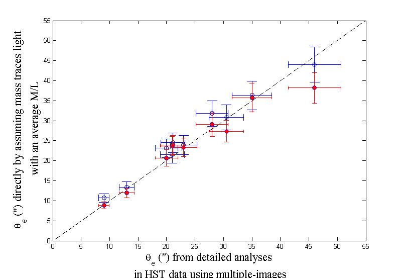
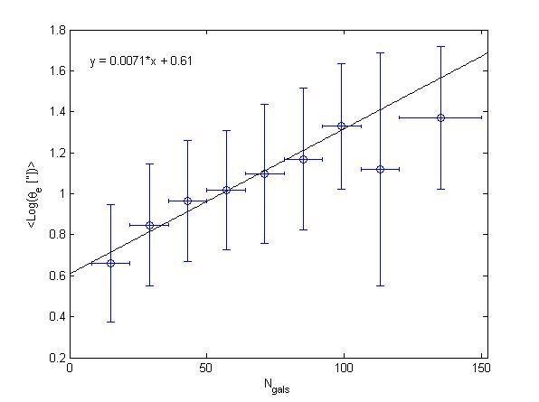
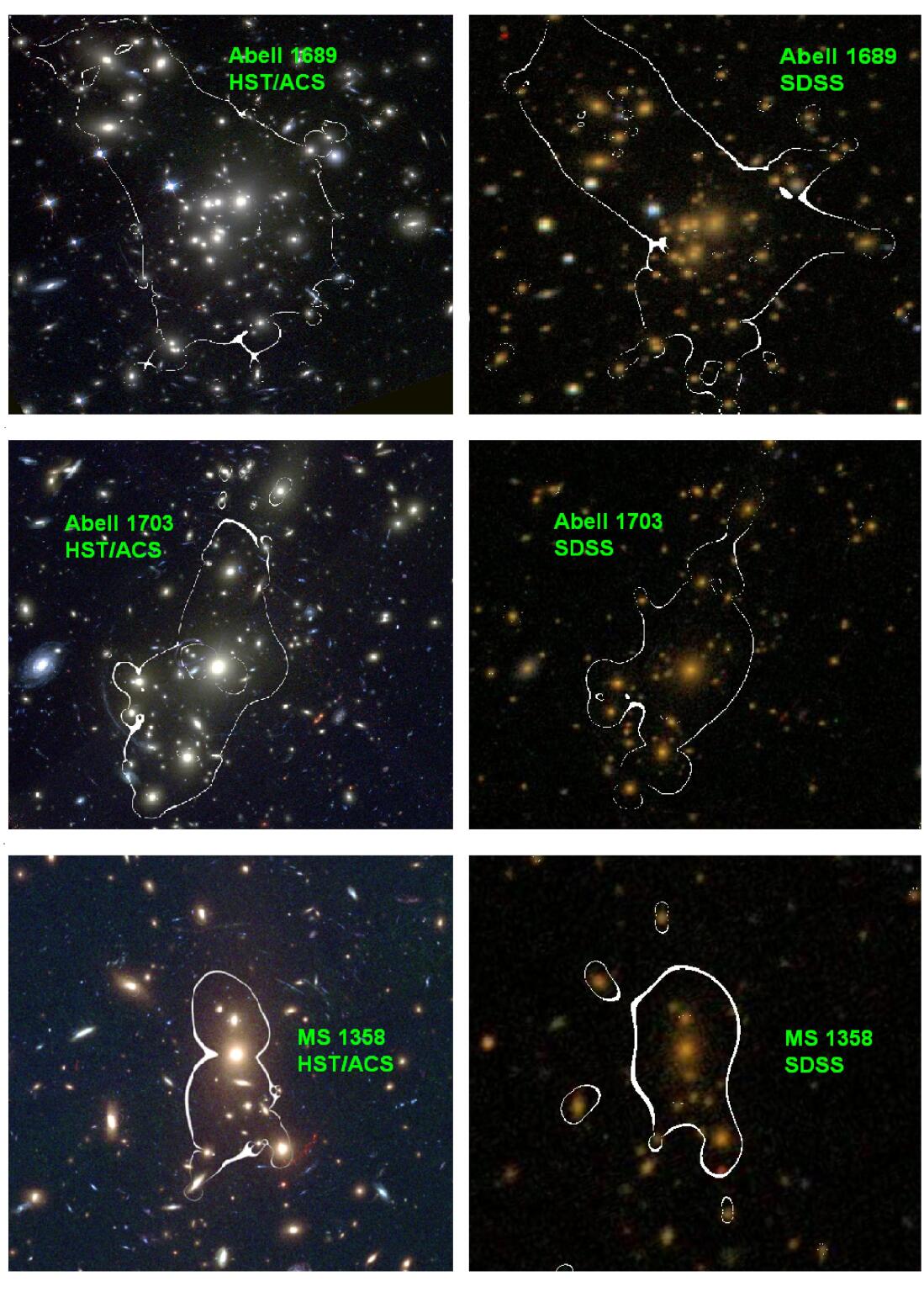
The incorporated method involves only four free parameters. Three of them are known sufficiently well a-priori and have only negligible effect on the critical curves and resulting Einstein radius, for which we adopt typical values deduced from detailed analyses of a few dozen clusters (more details are given in §2). The fourth parameter, which varies from cluster to cluster, is the overall (mass) normalisation, but since the respective distances are known, this can be simply overcome by finding a typical mass-to-light ratio () normalisation. The term is embedded, in practice, in a redshift-dependent normalisation factor, which is iterated for the best fit using 10 clusters which have been accurately-analysed in HST images and have parallel SDSS data listed in the Hao et al. (2010) catalog. These include some well-known lensing clusters such as A1689, A1703, MS1358, Z2701, and others (see, e.g., Broadhurst et al. 2005a, Richard et al. 2010, Zitrin et al. 2010, 2011a,b). The results of this comparison are shown in Figure 1 and Table 1.
The paper is organised as follows: In §2 we detail the modelling and the assumptions on which our algorithm is based. In §3 we discuss the results and relevant uncertainties, which are then summarised in §4. Throughout this paper we adopt a concordance CDM cosmology with (, , ). All Einstein radii referred to in this work are for a fiducial source redshift of . We also note that all logarithmic quantities in this work are in base 10, unless stated otherwise, and are denoted conventionally as “Log”.
2 Strong-Lens Modelling and Analysis
The method we apply here is based on the simple assumption that mass traces light. This well-tested approach to lens modelling has previously uncovered large numbers of multiply-lensed galaxies in ACS images of e.g., Abell 1689, Cl0024, 12 high- MACS clusters, MS1358, “Pandora’s cluster” Abell 2744, and Abell 383 (respectively, Broadhurst et al. 2005a, Zitrin et al. 2009b, 2011a,b, Merten et al. 2011, Zitrin et al. 2011c). As the basic assumption adopted is that light approximately traces mass, the photometry of the red cluster member galaxies is used as the starting point for the mass model.
2.1 Initial Mass Distribution
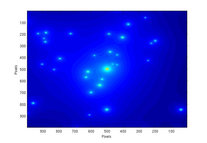
We now wish to calculate the deflection field by the cluster galaxies, or the initial mass distribution. By assuming that the flux is proportional to the mass, i.e., assigning a certain ratio, the deflection field contributed by each galaxy can now be calculated by assigning a surface-density profile for each galaxy, , which is integrated to give the interior mass, . This results in a deflection angle of (due to a single galaxy):
| (1) |
or more explicitly by inserting from above:
| (2) |
We note that all quantities are known, except for , the normalisation factor which is related to the M/L ratio (note that is maintained constant on a typical and known value, see §2.3). Thus, finding the explicit term for which scales correctly all clusters we analysed to date (taking into account the different lens and source redshifts) allows us - in principle - to perform the automated survey of Einstein radii, following the procedure described below.
By defining we can reduce the latter formula to get:
| (3) |
where also depends on the redshifts involved, and on the power-law index, (which is set to constant throughout, §2.3).
The deflection angle at a certain point due to the lumpy galaxy components is simply a linear superposition of all galaxy contributions scaled by their luminosities, (in units):
| (4) |
In practice we use a discretised version of equation 4, over a 2D square grid of pixels, given by:
| (5) |
| (6) |
where is the displacement vector of the th pixel point, with respect to the th galaxy position .
Note that to obtain the luminosity of each member, we convert its SDSS -band luminosity to the corresponding (Vega) B-band luminosity by the LRG template given in Benítez et al. (2009).
From these expressions a deflection field for the galaxy contribution is easily calculated analytically as above, and the mass distribution is now rapidly calculated locally from the divergence of the deflection field, i.e., the 2D equivalent of Poisson’s equation. An example is given in Figure 2.
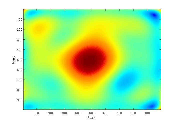
2.2 The Dark Matter Distribution
The mass contribution of galaxies is anticipated to comprise only a small fraction of the total mass of the cluster, which is expected to be dominated by a smooth distribution of DM. We now simply assume that the galaxies approximately trace the DM. As mentioned, this assumption was found to work very well in earlier work on many clusters where large numbers of multiple-images were found accordingly. These multiply-lensed systems are not simply eye-ball candidates, but are reproduced and predicted by the preliminary model, indicating that this model, based on the assumption that light traces mass, is initially well constrained.
Since the DM is of course expected to be smoother than the distribution of galaxies, we smooth the initial guess of the galaxy distribution obtained above, choosing for convenience a low-order cubic spline interpolation, typical to the many previous analyses mentioned above. The smoothing degree (the polynomial degree, ) is also a free parameter of the model, and the deflection field contributed by the DM is then simply the sum of the contribution from each point (or pixel) in this smooth DM component. This smoothing procedure is the key to our method’s success in locating multiple-images, and is in practice more useful than assuming a general DM shape such as NFW or pseudo-isothermal spheres, which are highly symmetric and do not necessarily describe the complex inner DM distribution in detail, often not allowing to find in advance the multiple images according to the initial mass distribution. An example of a smoothed component is shown in Figure 3.
The deflection field of the DM is then (where each pixel is treated as a point mass) given by:
| (7) |
| (8) |
where represents the (unnormalised) mass value in the th pixel of the smooth component. We therefore obtain now the deflection field due to the DM, hereafter .

2.3 The Total Deflection Field
Having calculated the two components of the deflection field, we now simply combine them to get a total deflection field as follows:
| (9) |
where is the relative contribution of the galaxy component to the deflection field.
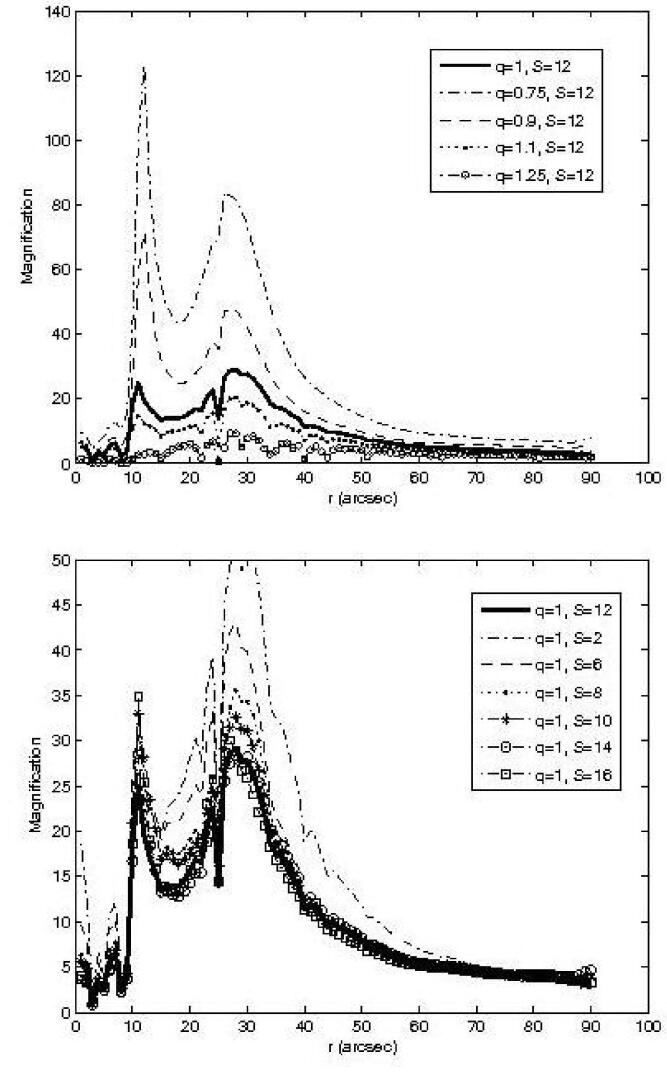
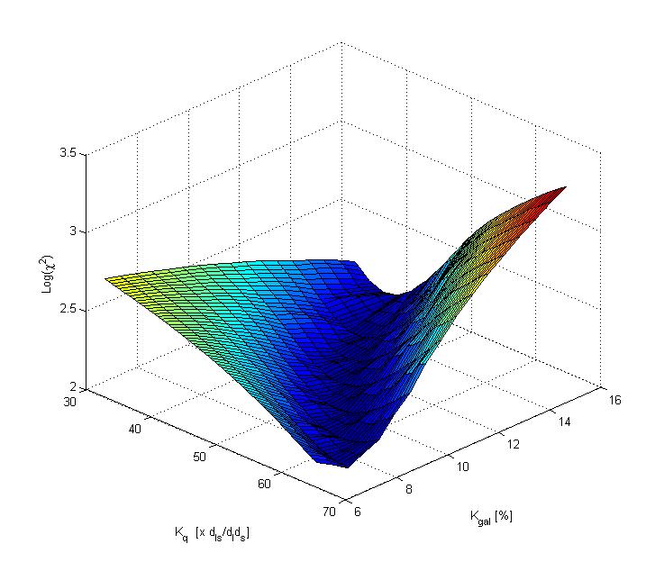
Both components of the deflection field are normalised by , so that knowing its value enables us to approximate very well the overall deflection field. It should be stressed that although the degree of smoothing () and the index of the power-law () are the most important free parameters determining the mass profile, their effect on the Einstein radius is negligible. Based on the detailed analysis of clusters (mentioned above and several more still unpublished), we note that the best-fitting parameters and show relatively little scatter among the different lenses. We can securely determine that the power-law will be in the range , and the smoothing polynomial degree will be in the range , with a sufficient resolution of and , in order to expand the full plausible profile range per cluster. More importantly, the exact choice of and does not affect the deduced Einstein radius size, which is determined by the inner mass enclosed within it and not by the mass profile which varies (see Figs. 1 and 2 in Zitrin et al. 2009b). The crucial point to make here is that Einstein radii just constrain the enclosed mass, no matter how the mass is distributed. This is seen very clearly in Figure 4 here, where we show that for many different combinations of the and parameters, the critical curves form at the same radius, given a reliable constraint. For example, in Figure 4 the critical curves were constrained using multiple-images, while our point here, in this work, is to show that the ratio deduced from a calibration sample can be used as an alternative constraint, enabling an automated SL analysis. In addition, it is therefore clear, that the choice of and parameter values is not fundamentally important here, and any combination, after it is calibrated for, should in principle yield the critical curves at the right location.
With this in mind, throughout the analysis here we maintain and constants with =1.2 and =10, which are typical values according to our many previous analyses. With and kept constants at these values, we now constrain the fixed value of the weight of the galaxies relative to the dark matter, , and the overall normalisation factor, . Having 10 clusters as a reference sample, and 2 parameters to constrain, we can well determine their values by a joint minimisation, and in turn examine how these best-fit values reproduce the reference sample critical curves. Explicitly, we perform a minimisation by comparing the Einstein radii of the calibration sample, deduced from detailed analyses based on HST observations and identification of multiple-images (see also §1), with the results of the automated procedure presented here, operated on the same clusters in SDSS data:
| (10) |
where i goes from 1 to , for the ten calibration-sample clusters, and is taken as of the HST deduced values, which is a typical value for the uncertainties in SL modelling results.
The results of this minimisation are seen in Figure 5. As can be seen, there is a strong correlation between the two parameters, and , which are degenerate so that many combinations of these can yield a good solution. This is a crucial point to make, since this correlation shows that indeed the number of free parameters in our modelling can be effectively reduced to one. By fixing the relative galaxy weight () to its best-fit value, the model can now be constrained with one single parameter, namely, the -related parameter . To do this, we fit by a least-squares minimisation, a line to the minimum points (defined as lying within a =2.3 above the minimal ), thus obtaining the linear relation between them. The fit is very good, , reflecting the strong correlation, and from which the independent errors are derived (i.e., by the residuals around the minimal values). With this we obtain a best-fit (and errors) relative galaxies weight of , similar to the value expected based on our many previous HST analyses.
However, one cannot expect the power-law lumpy component to represent only the galaxies, nor the smooth component to represent solely the DM, so that trying to assess the true physical weight of each component would be unwarranted at present. One can only know for certain that the combination of the two with as the relative weight, yields a good solution. It should also be mentioned, that we make a prior assumption on the range of sensible values, so that the critical curves are not too smooth nor too lumpy. This is done by inspecting the resulting critical curves by eye, so that roughly, the degree of “complexity” of the critical curves is similar to that seen in the aforementioned HST-based analyses of some of the calibration-sample clusters, and in agreement with the general expectation for the (small) contribution of galaxies relative to the total mass.
For the normalisation factor, we obtain in the minimisation a best-fit value of ( errors). Accordingly, the related coefficient, , equals , in units of [; with =1.2], from which we can deduce the explicit typical relation:
| (11) |
where here, is in radians, and is the galaxy luminosity (in solar unit). For example, for a typical BCG as bright as , this yields an value of within , or e.g., within . Note that this is not the typical per galaxy, but overall, a scaling which describes, per , the total projected mass enclosed along the line-of-sight and within a cylinder of radius centred on a galaxy, and thus includes major contribution from the cluster DM halo along this line. Therefore, this term is coupled to the modelling procedure applied and include some internal rescalings and compensation to various effects such as the difference in the depth between the usual SDSS and HST imaging, and the red-sequence membership definition (§3), and are coupled to the LRG template and its possible minor redshift evolution (Benítez et al. 2009). In fact, here we do not explicitly take into account this evolution of red-sequence galaxies and their host clusters, so that the resulting relation presented here may include a compensation to this effect, which although is expected to be minor (Benítez et al. 2009), would be interesting to probe when a larger calibration sample is available.
With these best-fit values we analyse each of the SDSS reference-sample clusters sequentially in an automated way. The errors on these parameters mentioned above, propagate typically into a minor error on the Einstein radius (of each individual cluster of the calibration sample), which may be too low in light of other uncertainties detailed in §3; accordingly, a more realistic error (or uncertainty) level is estimated as mentioned therein. The resulting Einstein radii of the SDSS blind analysis are compared to the results of detailed analyses in Figure 1, where a very good correlation with a small scatter is found (, and deviation of less than ). A more explicit example of the analysis results obtained by the different approaches is given in Figure 14.
| Identifier | RA | DEC | ref | other refs | |||||||
|---|---|---|---|---|---|---|---|---|---|---|---|
| J2000.0 | arcsecs | arcsecs | arcsecs | ||||||||
| A1689 | 197.87295 | -1.3410050 | 0.2030 | 0.0180 | 0.1832 | 46.0 | 44.1 | 38.2 | 142 | Z | B05,HSP06,L07 |
| A1703 | 198.77197 | 51.817494 | 0.2690 | 0.0180 | 0.2800 | 28.0 | 31.8 | 29.0 | 86 | Z10 | L08,R09 |
| MS1358 | 209.96066 | 62.518110 | 0.3590 | 0.0290 | 0.3273 | 13.0 | 13.4 | 12.0 | 69 | Z11a | |
| MACS1423 | 215.94948 | 24.078460 | 0.4410 | 0.0950 | 0.5430 | 20.0 | 23.2 | 20.7 | 16 | Z11b | L10 |
| A1835 | 210.25886 | 2.8785320 | 0.2100 | 0.0390 | 0.2528 | 30.5 | 30.8 | 27.4 | 65 | R10 | |
| Z2701 | 148.20456 | 51.885143 | 0.1920 | 0.0210 | 0.2151 | 9.0 | 10.7 | 8.8 | 11 | R10 | |
| A611 | 120.23668 | 36.056725 | 0.2900 | 0.0160 | 0.2873 | 21.0 | 21.5 | 23.7 | 59 | R10 | D11 |
| RXJ2129 | 322.41651 | 0.089227 | 0.2280 | 0.0140 | 0.2339 | 21.1 | 24.5 | 23.9 | 25 | Z | R10 |
| A963 | 154.26499 | 39.047228 | 0.2230 | 0.0110 | 0.2056 | 23.0 | 23.9 | 23.3 | 50 | Z | R10 |
| A2261 | 260.61326 | 32.132572 | 0.2250 | 0.0120 | 0.2233 | 35.0 | 36.3 | 35.8 | 74 | Z | U09, C12 |
3 Results, Discussion, And Uncertainty
The sample analysed in this work is drawn from the Hao et al. (2010) SDSS cluster catalog. As mentioned in their work, Hao et al. (2010) have developed an efficient cluster finding algorithm named the Gaussian Mixture Brightest Cluster Galaxy (GMBCG) method. The algorithm uses the Error Corrected Gaussian Mixture Model (ECGMM) algorithm (Hao et al. 2009) to identify the BCG plus red sequence feature and convolves the identified red sequence galaxies with a spatial smoothing kernel to measure the clustering strength of galaxies around BCGs. The technique was applied to the Data Release 7 of Sloan Digital Sky Survey and produced a catalog of over 55,000 rich galaxy clusters in the redshift range . The catalog is approximately volume limited up to redshift and shows high purity and completeness when tested against a mock catalog, and when compared to other well-established SDSS cluster catalogs such as MaxBCG (Koester et al. 2007; for more details see Hao et al. 2010).
We go over the Hao et al. (2010) catalog, and apply the method described above (§2) to each cluster, deriving its resulting Einstein radius and mass. We present here the results from the first 10,000 clusters analysed. In practice these 10,000 SDSS clusters comprise only a relatively small fraction () of the full catalog coverage, whose analysis results we aim to presented in a future work, once a larger calibration sample is available.
3.1 Einstein Radius Distribution
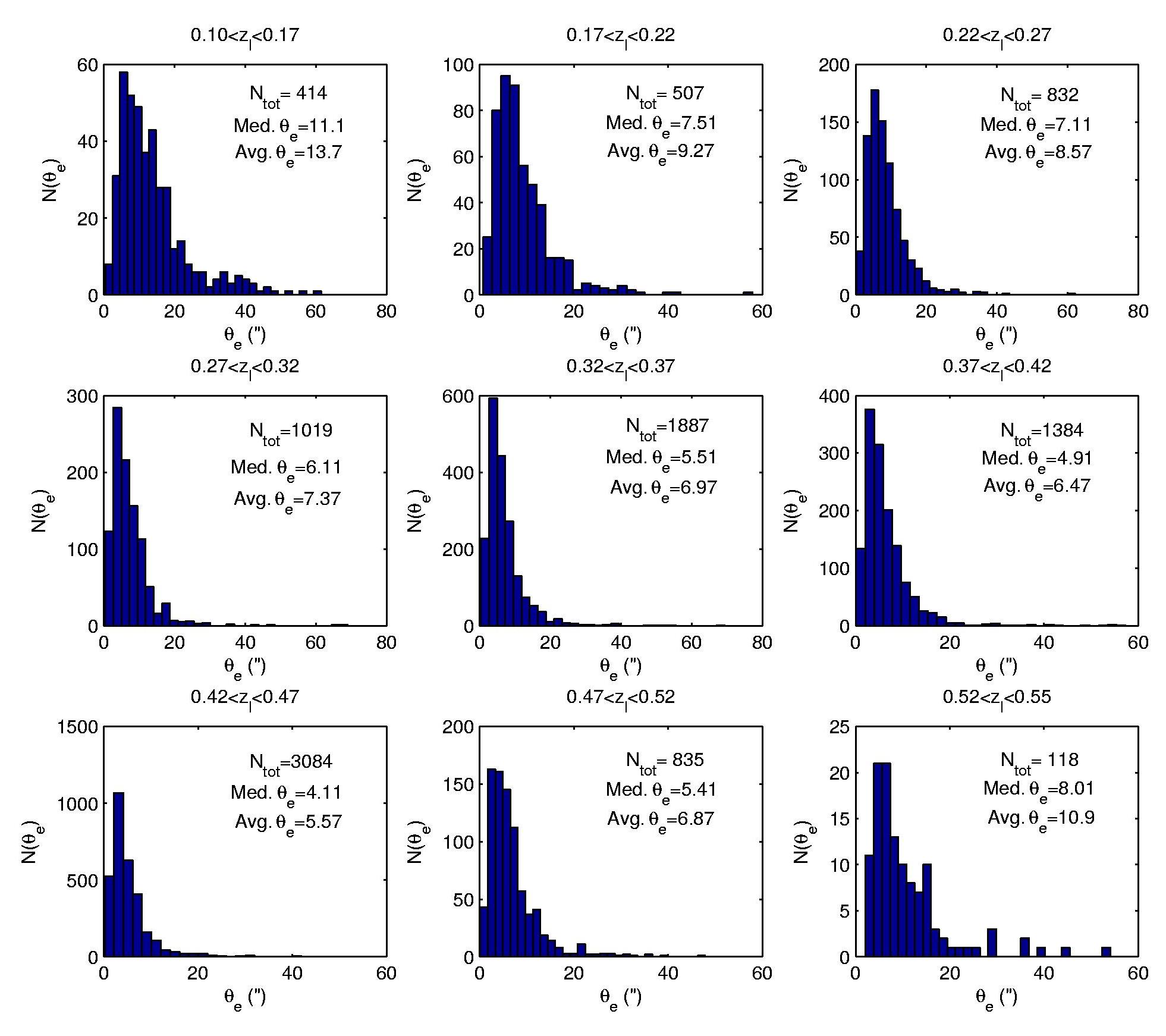
The resulting Einstein radius distribution for this sample is seen in Figure 6 as a function of lens redshift (for constant ), along with the average and median Einstein radii for each redshift bin, which evolve in redshift and peak at (for ), as may be generally expected given the hierarchical growth history of clusters and the distances involved in lensing (this is further discussed in §3.3). The Hao et al. (2010) cluster catalog lists clusters with at least 8 members within 0.5 Mpc from the BCG. This low limit results in a realistic domination of galaxy-scale lenses ( of an order of a few arcseconds), which are usually not massive enough to form impressive lenses with large Einstein radii and many multiple-images. The more interesting information may be the higher end of the distribution at larger radii. The concept of the largest Einstein radius in the Universe and the expected abundance of large lenses have been discussed thoroughly in the literature, and are especially of high interest as they teach us about the reliability of the standard CDM model in predicting these extreme cases, as the CDM model does not favor the formation of giant lenses (e.g., Broadhurst & Barkana 2008, Sadeh & Rephaeli 2008, Zitrin et al. 2009a).
Note that clusters with large Einstein radii are found also towards higher redshifts. In addition, though not included in this work, the largest known lens to date, MACS J0717.5+3745 is at a similarly high redshift of , with for (see Zitrin et al. 2009a). Due to a very shallow mass distribution in this cluster (Zitrin et al. 2009a), for the Einstein radius will be only slightly lower, around (see also recent paper by Limousin et al. 2011 for new redshift information for this cluster). The exact number will be derived elsewhere, in the framework of the CLASH program. The abundance of larger lenses at these redshifts is caused usually (e.g., Zitrin et al. 2011a), by a spread-out, unrelaxed matter distribution. At these higher redshifts many clusters are not yet relaxed and still undergo mergers, so that the mass distribution is already sufficiently dense for significant lensing, but widely-distributed so that the Einstein radii of the different substructures are merged to form extended critical curves (e.g., Torri et al., 2004, Dalal, Holder, & Hennawi 2004). On the other hand, at a lower redshift, more concentrated clusters are those yielding larger Einstein radii, as there is more mass in the centre enhancing the critical area (see also §3.3).
The blind analysis performed here yielded initially 69 candidates with (), many coincident with various Abell or MACS clusters. We visually inspect each of these clusters and find that some are boosted by various effects detailed below (we omit these clusters from our further analysis), but infer that at least about half of these are most likely real giant-lens candidates, with a maximum of () for the most massive candidate. We direct the reader to works by Hennawi et al. (2007a) and Oguri & Blandford (2009) which have investigated in detail the Einstein radius abundance on various scales, based on simulations and CDM expectations, and taking into account triaxialities which induce a prominent lensing bias.
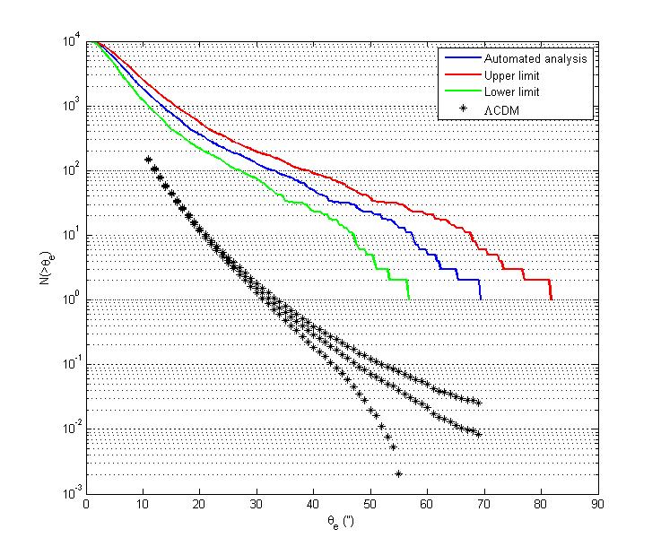
Our realistic, observationally-based results free from lensing bias, are compared to some such expectations explicitly in Figure 7, where we plot the cumulative distribution of clusters above each radius with the expected errors, propagated from the errors on the best-fitting parameters as described in §3.2. Note, the lower limit shifts the maximal Einstein radius from to (), close to that of the largest known lens, MACS J0717.5+3745 (Zitrin et al. 2009a). We note that Oguri & Blandford (2009) who examined in detail the Einstein radius distribution based on semi-analytic expectations, have derived maximal Einstein radius values of , but these as shown in their work are very susceptible to the cosmological parameters in general and to in particular, and can reach (within the confidence) values that are nearly twice as high. Their expected distribution, scaled to the same sky area as our sample and with WMAP7 parameters (Komatsu et al. 2011), is overplotted in Figure 7. Aside for an agreement between their expected largest Einstein radius and the largest lenses found in our analysis, the two cumulative distributions clearly disagree. Although normalised to the same effective sky area, there is a order-of-magnitude number difference for small Einstein radii, which reaches a orders-of-magnitude difference for higher Einstein radii, so that in addition, the two distributions have also different slopes. The origin of the discrepancy is not clear, but part of the difference may be due to a different (lower) mass limit probed by the two methods. In addition, the effect of the concentration-mass () relation and the chosen mass function used in semi analytic calculations should clearly have a strong influence on the resulting distribution (e.g., Duffy et al. 2008, Macció et al. 2008, Prada et al. 2011; for differences among various relations), as higher concentrations entail higher inner mass and Einstein radius. We leave the examination of how these may influence the cumulative distribution, for future work.
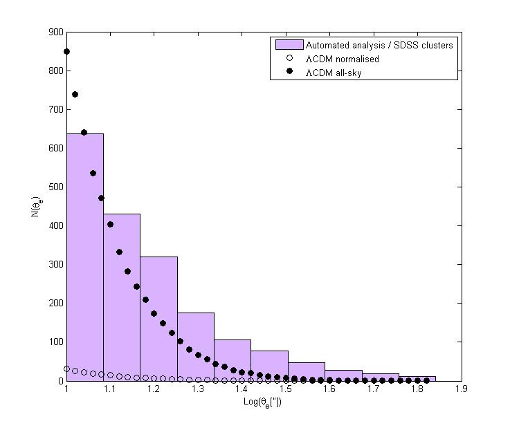
To assess the difference from the semi-analytic expectation by Oguri & Blandford (2009; see also Figure 7), we compare the width of the tails for , which is the lower limit taken in their calculation. As can be seen in Figure 8, both distributions are (semi) log-normal although with two main differences. The Oguri & Blandford (2009) distribution has a width of (in ), while our distribution shows a slower (or wider) decrease, with . This difference is commensurate with the different decline of the cumulative distribution seen in Figure 7. Also, the overall number of clusters in their analysis, for the same sky area, is much lower, although this may be, as mentioned, entailed by the different mass limits probed by each method, which will be checked in future work. As mentioned above, one of the most interesting aspects of our study, namely the largest Einstein radius, is in good agreement with the estimation by Oguri & Blandford (2009).
3.2 Uncertainty and Error Estimation
Various factors of error should be taken into account when addressing the results reported in this work, though these are mostly statistical and therefore due to the extensively large sample are not significant. In addition, these uncertainties arise mainly from the data themselves, so that applying the method presented here to higher-end, dedicated cluster-survey data (e.g., the expected J-PAS survey; Moles et al. 2010), should produce much cleaner results.
3.2.1 Possible Factors of Error
The first error factor we have investigated is the lens photometric-redshift error. The typical photo- uncertainty for the sample BCGs (by which we determine the lens distance) is 0.015. A error in the lens redshift can be translated into a noticeable () difference in the measured Einstein radius, and only about half of the sample has spectroscopic redshifts for the BCG, thus the results for some of the clusters are affected by this error. As can be seen in Hao et al. (2010), the photometric redshifts were tested against the spectroscopic redshifts where possible, yielding a very tight relation strengthening the confidence in them. We have tested the effect of the photometric redshifts on the calibration sample, and regenerated Fig. 1 based on the photometric redshifts (instead of the spectroscopic redshifts; see also Table 1). Only slight differences are seen and the overall scatter remains essentially the same. To assess the effect of the photo- error more quantitatively, we analysed a sample of 500 random clusters (detailed in §3.2.2) with the catalog photometric redshifts, and then repeated the analysis by photometric redshifts drawn randomly from a normal distribution centred on the catalog photometric redshift for each cluster, with a width of (which is the photo- error quoted in Hao et al. 2010). From this we indeed obtain a low uncertainty of only on the cumulative Einstein radius distribution, and for the differential (log-normal) distribution, differences of only and on and , respectively.
Second, the SDSS imaging is shallower than typical HST imaging dedicated to SL analysis. Correspondingly, and supplemented by the conservative cluster-finding algorithm, some of the cluster members are overlooked and often not associated with the cluster, and only the brighter galaxies are incorporated. Luckily, these are also the more massive galaxies and thus the effect on the lens model is minor. In addition, the inclusion of (less-massive) cluster members is known to affect locally the shape of the critical curve, but not to change their overall size (e.g., Flores, Maller & Primack 2000, Meneghetti et al. 2000). The constant which was iterated for (which includes the ratio) is probably boosted by the relative loss of galaxy mass-representations in our modelling of the SDSS catalog. This, however, can be very well assumed to be a relatively constant ratio and thus, along with the intrinsic scatter, does not affect substantially the results, as can be seen in the calibration sample comparison, where a clear consistency is found. This may not at all be surprising, since the modelling here is based on simple physical considerations: it has been well established that light approximately traces mass, and clearly, a reasonable relation can be incorporated.
Another factor of possible contamination is the lower resolution of SDSS images compared with typical lensing images by HST. This we find may result in local overestimation of the BCG, if another cluster member is found too close to the BCG core to be resolved, thus boosting the Einstein radius (and mass), especially for higher-redshift lenses. The reason is that the smoothing procedure, or the (2D polynomial) fit, is dominated by the BCG. Therefore, although the lumpy (galaxy) component in such scenarios should not have a substantial effect, the smooth component will be over-boosted in the middle (since the BCG would be too bright), thus pushing outwards the Einstein radius. However, this chance alignment is naturally not too common, and in any case will affect mostly the lower end of the distribution, i.e., clusters with small Einstein radius that is dominated fully by the BCG. Clusters with large Einstein radii will be less susceptible to such contamination as the critical curves are not fully dominated by the BCG and contain substantial contribution from other massive cluster members as well.
A known factor of systematic error considered in related work on various samples of (often SDSS) clusters, is the miss-centring of mass with respect to the BCG (e.g., Becker et al. 2007, Johnston et al. 2007a, Rozo et al. 2009,2010, Oguri & Takada 2011). In that sense, methods which depend on a predefined centre may be affected from a scatter in the location of the BCG with respect to the true centre-of-mass, if the prior is constantly assumed to lie at the very centre of the cluster. However, in our method, there is no need to predefine the exact centre-of-mass. The smoothing procedure we implement has the advantage of being independent from a predefined centre, and the result is ultimately determined simply and directly by the galaxy (light) distribution. In fact, this has enabled us to find various such shifts between the BCG and the centre of (dark) mass (e.g., Zitrin et al. 2009b, Umetsu et al. 2011a).
However, if the GMBCG catalog itself has misidentified a galaxy as the BCG, which we use as the centre-of-frame for our analysis, this may entail a shift in the analysed field, so that in principle some relevant galaxies may lie outside it. Nevertheless, since the Hao et al. (2010) catalog considers galaxies within 0.5 Mpc, even for the highest redshift clusters of the sample (), this size translates into arcseconds. Since the Einstein radius is determined by the mass enclosed within it, and since only less than a handful of clusters may have such a large Einstein radius (following the upper limit, see Figure 7), this may only have a negligible effect over the whole sample.
It should be noted that the results for should be more cautiously addressed, as the catalog is officially volume limited up to this redshift due to the luminosity cuts that require potential member galaxies to be brighter than 0.4L*, where L* is the characteristic luminosity in the Schechter luminosity function. Also, for higher redshifts, the different red-sequence criteria ( instead of , see Hao et al. 2010) may come in play and input some more noise, mostly with respect to the richness level, so that overall one should expect fewer members assigned for clusters relative to clusters below this redshift. In order to test this effect we repeated our analysis including only clusters in the volume limit of and verified that only negligible differences are seen with regard to the Einstein radius distribution (e.g., such analysis yields a log-normal Einstein radius distribution with and , similar to the full sample; see Figure 9). In addition, high redshift clusters in the calibration sample also show a satisfying result following the same scaling relation as lower redshift clusters (with a scatter of up to with the best-fitting parameters, or up to scatter with the Jackknife minimisation, see §3.2.2). Also, if we exclude these from the calibration-sample minimisation, the best-fitting parameters differ by less than from those obtained with the full sample.
We have identified within the 69 initial candidates with (), several clusters that were misidentified as higher redshift clusters (according to their observed BCG), though they are most likely substructures of a foreground more massive (and known) cluster on the same line-of-sight. This boosts significantly the Einstein radius, and such cases as mentioned were omitted from our further analysis. Due to the low chances of such alignments and resulting misidentifications, the effect of this on the full sample and especially on the lower regime, is expected to be minimal.
3.2.2 Quantification of Errors and Uncertainty
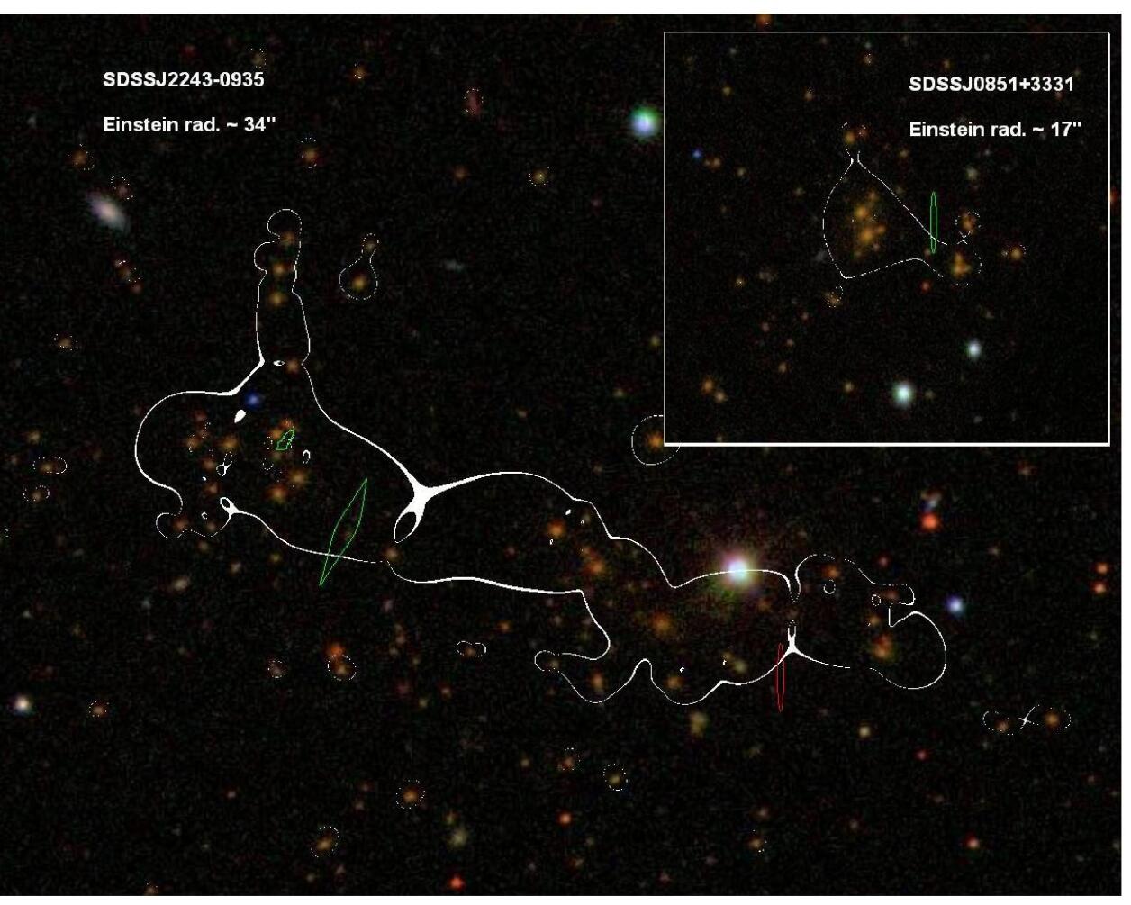
In order to assess better the amount of statistical uncertainty caused by the various factors (e.g., §3.2.1), we have first examined by eye a sample of 100 random clusters from the catalog and the critical curves generated for them by our automated modelling. We found only 3 clusters whose Einstein radius is boosted due to an unresolved galaxy near the BCG, and 15 more clusters with some galaxies that by eye do not necessarily seem to have similar colors, so that if these are misidentified as cluster members, may be introducing some additional noise. Clearly, this designation is not purely objective, but still allows us to conclude, in addition to the other consistency checks we performed, that the overall noise level in our analysis is reasonable. As an additional complementary step, and regardless of the calibration sample, we searched for SDSS arcs found in Bayliss et al. (2011b) and examined how well our critical curves could in principle reproduce these (giant) arcs. Although the location of the arcs is not used as input, our blind analysis automatically reproduces critical curves that pass through them as expected, strengthening further our automated approach. An example is given in Figure 15.
To explicitly quantify the errors and level of uncertainty we perform two majors procedures. Firstly, we perform a “Jackknife” minimisation: on top of the (eq. 10) minimisation with the full calibration sample (to find the best parameters for the blind analysis), we perform the minimisation 10 more times, each time omitting one cluster from the fit, and then analysing it with our automated procedure to examine how well the Einstein radius is estimated. We note, that by doing so the best-fit values for and in each such iteration distribute around the best-fitting parameters when minimised by all ten clusters together, with values up to away. With this, we obtain that the Einstein radii for all ten clusters are estimated within of their reference value (according to HST-based detailed analyses with multiple-images as input), while 9 clusters show a scatter of up to . These (only) represent how well each of the Einstein radii of the calibration sample can be reproduced individually.
Therefore, secondly, we wish to examine how the () errors drawn from the full reference sample minimisation are propagated into the statistical results, since these should depend on other quantities such as, e.g., the number of lenses per (Einstein radius) bin. For that purpose, we analyse 500 random clusters with the best-fitting parameter values, and then repeat the analysis marginalising over the errors. For the differential, log-normal Einstein radius distribution, these result in differences of on , and on , and upper and lower limits of on the cumulative Einstein radius distribution (Fig. 7). We take these to represent the level of (statistical) uncertainty in our analysis.
It should be mentioned, that although the sample analysed here was not selected based on mass or arc abundance and thus is not biased in terms of lensing, the calibration sample used to determine the model parameters ( in particular) consists of 10 well-known massive clusters, which might introduce a systematic error boosting the Einstein radii. Though low and moderate-mass lensing clusters are hard to model for comparison due to lack of multiple-image constraints, the calibration sample contains clusters with as few as 11 members, and as many as 142 members, thus spanning nearly the full richness range of the probed SDSS sample. The possible bias might be further looked into by comparing galaxy and group-scale lenses with known prominent arcs, often found in systematic surveys for gravitational arcs (e.g., Sand et al. 2005, Hennawi et al. 2008, Kubo et al. 2010, Bayliss et al. 2011a,b, Wen, Han & Jiang 2011), which should also be useful for extending the calibration sample and examining further this effect.
We note that due to the approach implemented here which does not use multiple-images as input, the profiles and magnifications are not well constrained for each cluster, and the only relevant measure which we refer to is the effective Einstein radius (and enclosed mass), as seen in Figure 4. Naively, one could in principle derive the mass profile for each lens by simply assuming different fiducial source redshifts and calculate the enclosed mass by implementing their distance-redshift relation, but this would be premature at this stage, as though the parameters maintained constant here (on typical values) do not considerably affect the critical curves shape and size, the mass profile is susceptible to these and thus a separate calibration is required for each source redshift based on the full reference sample. This however may indeed be plausible, as we intend to probe in future work.
3.2.3 Consistency checks
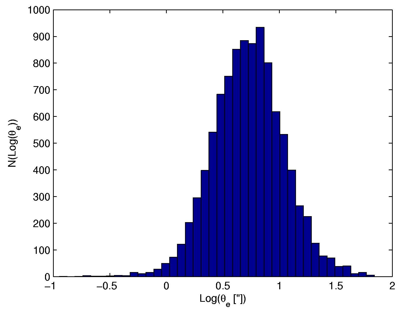
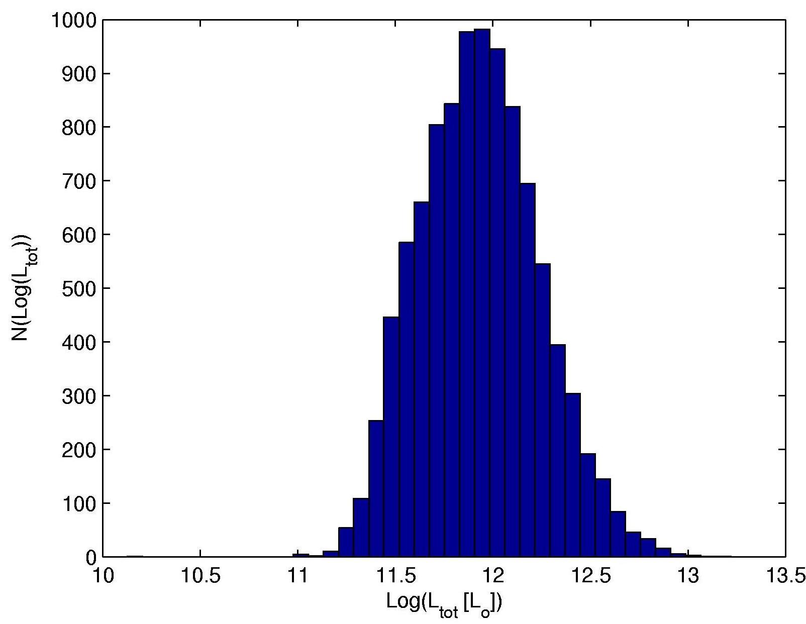
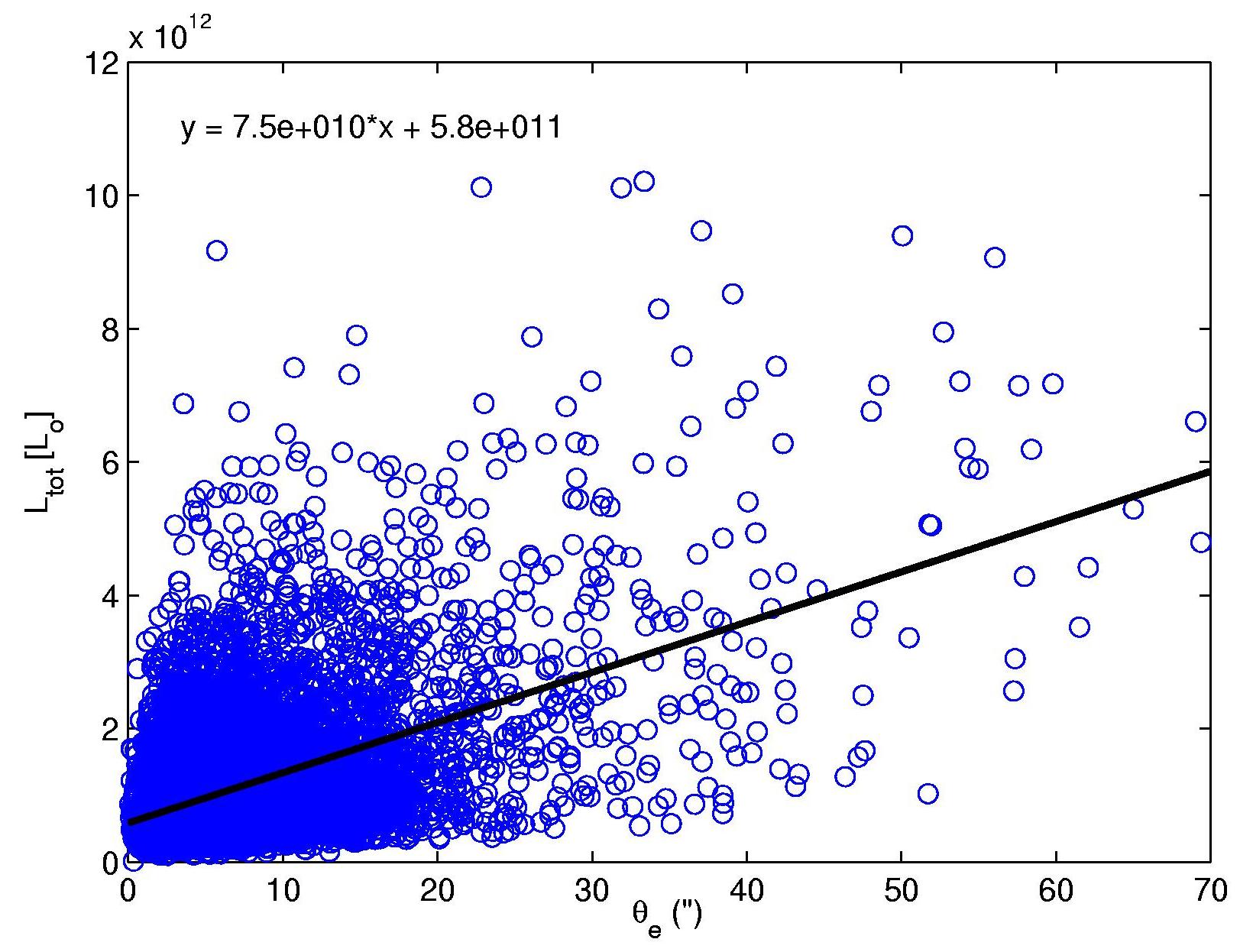
To further verify that the data used here is reasonable for our purpose, especially the luminosity of clusters members to which our method is coupled, we perform a few simple self-consistency checks. The overall Einstein radius distribution is plotted is Figure 9, and is clearly log-normal in shape, with and . The luminosity distribution is plotted in Figure 10 for comparison, and for each cluster we explicitly compare in Figure 11 the total luminosity to its resulting Einstein radius, where it is importantly evident that the total luminosity itself is not an accurate enough measure of the Einstein radius. Following a more realistic procedure as described in this work is necessary in order to obtain a reliable mass and Einstein radius distribution. More explicitly, as the mass is more concentrated than the light, one must choose a more concentrated representation for the galaxies (e.g., the power-law used here), which is then simply scaled by the luminosity. Similarly, we stressed that the DM is well represented by smoothing the galaxies mass distribution, which is more efficient in practice for the inner SL region, than e.g. assuming a symmetric mass distribution such as NFW which often does not allow to immediately uncover the multiple-images by the model.
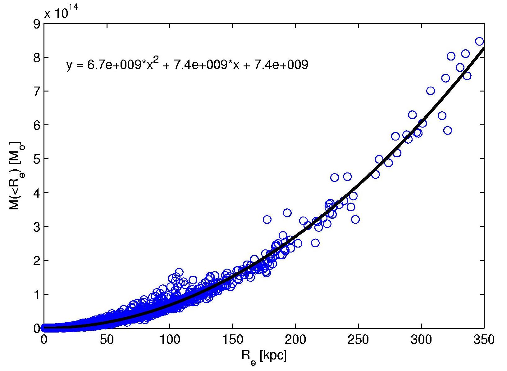
In Figure 12 we plot the enclosed mass versus the Einstein radius for each cluster. Although a tight relation is expected directly from the lensing equations, this constitutes an important self-consistency check. We simply measure the Einstein radius for each cluster as the area enclosed within the critical curves (exploiting the magnification sign-changes to estimate this automatically), where the mass is measured by summing the surface-density in the pixels which fall within the critical curves. The Einstein masses correlate well with the Einstein radii, with a square relation as expected, and with a reasonable scatter since the clusters cannot be expected to be strictly symmetric. Explicitly, the of the fit is 0.985, and the mean scatter is lower than (although there is an excess in the scatter of up to almost around 100 kpc for some individual clusters, probably due to the different factors of error elaborated in §3.2.1). Also, in this consistency check, clusters spuriously assigned with large Einstein radii due to effects detailed above did not follow the expected relation, aiding us to exclude them from our further analysis.
3.3 Correlations with cluster parameters
Since the Einstein radius correlates with the mass interior to it, some dependence on the examined cluster parameters which are related to the observed mass, such as redshift, richness, and luminosity, can be expected. For example, in Figure 6 we showed the Einstein radius distribution in different redshift bins, where it is evident that large Einstein radii are observed more frequently in the lower () and higher () redshifts of the sample, whereas in intermediate redshifts the mean Einstein radius is smaller.
To further quantify this effect, and since Figure 9 shows that the Einstein-radius distribution is log-normal, we plot the mean (and width) of the log-normal effective Einstein radius distribution in different redshift bins. The result is seen in Figure 13 (top), where we also fit first- and second-order polynomials to the data. Although this tendency is only of the order of the log-normal distribution widths, the mean effective Einstein radii steadily decrease from to , and then increase again (see Figure 13). This tentative decrease of the mean effective Einstein radius with redshift may be related to cluster evolution. For example, lower redshift clusters, which have had more time to collapse, relax, and virialise, are expected to have more concentrated mass distributions and thus be stronger lenses (e.g., Giocoli et al. 2011). On the other hand, the tentative increase of the mean effective Einstein radii towards may be related to more substructured mass distributions, whose critical curves for the several merging subclumps are merged together to a bigger critical curve (e.g., Torri et al., 2004, Dalal, Holder, & Hennawi 2004), although it is unclear at present how prominent is this effect.
It should be noted, however, that the cluster catalog is volume limited only up to where the tentative rise with redshift towards larger Einstein radii sets in. No weight should therefore currently be given to the two highest redshift bins since they may be affected by different selection criteria applied for cluster detection above . To test this, we examined plots of the cluster luminosity and richness versus redshift, as larger clusters should have in principle higher luminosity and richness. A pronounced step is seen at , so that the majority of luminous clusters () is found at , which most likely renders the rise in Einstein radii above a result of the different red-sequence criteria applied for higher- clusters. Given this, we ignore the mean effective Einstein radii above , and concentrate on the indication of a decrease from low redshift towards .
One should quantify the effect of geometry on the observed evolution of the mean (log) Einstein radius with redshift. The motivation is to check what is the contribution of pure geometrical effects, versus, say, evolutionary processes of the clusters. However, this can only be done qualitatively, since in order to know the geometrical dependence of the Einstein radius, one has to know the mass profiles in advance. For example, for a point mass , while for an isothermal sphere . Generally, for a power-law projected mass distribution , the angular Einstein radius scales with the distances as . If we take the power law to be isothermal, , the angular Einstein radius (for constant ) decreases by from the bin to the bin. For mass profiles steeper than isothermal, decreases more rapidly with lens redshift, while for flatter profiles it increases (or shows a more complex behavior such as increasing and then decreasing). The observed monotonic decline between and seen in Figure 13 is of , so that a steeper profile than isothermal () is needed to fully explain this decline by geometrical means. Any possible significance of the redshift evolution of for cluster evolution can thus only be assessed once the mass profile is known.
We also compare the observed decline to semi-analytic calculations, in which standard concentration-mass relations and mass functions are incorporated. Quite independent of their detailed assumptions, such calculations yield increasing mean Einstein radii with lens redshift, opposite of our result. One such semi-analytic calculation we use for comparison here (M. Redlich, private communication) is based on the Press & Schechter (1976) mass function. Effective Einstein radii are derived from assumed relaxed (i.e. non-merging), triaxial NFW haloes, adopting the concentration-mass relation from Jing & Suto (2002) and including only halos with . This calculation yields, similar to the result by Oguri & Blandford (2009), a larger fraction of smaller Einstein radii than our findings, and the mean effective (logarithmic) Einstein radius increases with redshift, contrary to the decline we observe here. This however, may be partly explained (like the discrepancy in Figure 7) by the lower-mass limit (more lower-mass clusters in higher redshifts would alleviate the discrepancy), or the choice of mass function and concentration-mass relation implemented therein. A more extensive calibration sample needs to be obtained before strict conclusions can be drawn. In principle, however, our results may help to pin down the true concentration-mass relation, in order to be compared with the evolution trends obtained in semi-analytic calculations, independent cluster evolution studies (e.g., Maughan et al. 2008 and references therein), or related numerical simulations (e.g. Duffy et al. 2008, Macció et al. 2008, Prada et al. 2011).
Finally, we note that the (logarithmic) mean effective physical Einstein radius, i.e. the angular Einstein radius times the angular-diameter distance to the cluster, is constant across the redshift range with kpc. Tentatively, near-constant physical Einstein radii with redshift can be achieved with standard, e.g. NFW density profiles if the concentration-mass relation evolves steeply with redshift. Adopting a relation of the form (e.g. Duffy et al. 2008), we find that is required to reproduce the trend seen in Figure 13. Current well-established concentration-mass relations extracted from numerical simulations find (e.g., Bullock et al. 2001, Duffy et al. 2008). We emphasize once more that these conclusions are tentative and preliminary, as the results of this work should be revised once a more significant calibration sample is available. A more profound investigation of the indicated redshift evolution and its comparison to numerical simulations would thus be premature.


Apart for the redshift dependence, we repeated the above procedure and examined the mean effective logarithmic Einstein radii also in different total luminosity and richness bins (namely, how many red sequence galaxies are assigned to each cluster by the Hao et al. 2010 catalog). The evolution of and for these is plotted in Figure 13 (centre and bottom), respectively. A (mild, given the distribution widths) trend is uncovered as a function of both luminosity and richness, so that on average, higher luminosity and richness clusters, show larger Einstein radii. These trends are quite expected, since richer clusters are naturally more luminous and more massive, correspondingly (for established mass-richness relations see, e.g., Rozo et al. 2009, Bauer et al. 2012). In addition, although not specifically shown here, for completeness we also examined both the richness and luminosity in the difference redshifts bins. We note that the richness is constant throughout the volume-limited redshift range, while monotonically increases by from to , as can be generally expected from passive evolution of the cluster galaxies (although also here the trend is insignificant given the widths of the distribution in each bin, which is of the same size as the increase throughout the range, ).
We note, in addition, that with respect to the widths of the logarithmic distributions in different redshifts, luminosity or richness bins, we do not uncover any prominent trend (which could withhold information on, say, the level of different population mix in the different bins).
4 Summary
In this paper we presented an automated strong-lens modelling tool, which is used to efficiently derive the Einstein radius and mass distributions of 10,000 SDSS clusters, found by the Hao et al. (2010) cluster-finding algorithm in DR7 data. We adopt the well-tested approach that light overall traces mass (with a more realistic representation of the galaxies and DM, see §2), and normalise according to a typical average mass-to-light relation established here, to obtain a reliable deflection field based on the distribution and luminosity of bright cluster members.
This procedure, as we have shown in many previous SL analyses, is sufficient to derive the critical curves with enough accuracy to immediately identify many multiple-images across the lensing field, as the primary mass distribution is initially well-constrained. Here we used a subsample of 10 well-studied clusters covered by both SDSS and HST to calibrate and test our analysis method, and showed that remarkably accurate determination of the Einstein radius can be made in an automated way, based on the light distribution of bright galaxies, and scaled by their luminosity. A tight correlation is seen between the Einstein radii derived in detailed analyses of HST data and using multiple images as input, and those from the “blind” survey tool presented here, operated on the same clusters but in SDSS data and without using any multiple-images information as input.
This efficient modelling method enables us to present the first observationally-based representative Einstein radius distribution, based on a coherent unbiased sample of the first 10,000 clusters in the Hao et al. (2010) catalog, larger by a few orders of magnitude than the number of SL clusters analysed to date. For this all-sky representative sample the Einstein radius distribution is log-normal in shape, with , , and with higher abundance of large clusters than predicted by CDM, and with a maximum of () for the most massive candidate, in agreement with semi-analytic calculations.
In addition to characterising the overall Einstein distribution, we also uncover various relations with cluster properties listed in the probed catalog. For example, as may be expected, a clear relation is seen between the logarithmic Einstein radius distribution mean (for ), and the luminosity or richness, so that richer and more luminous clusters exhibit, on average, larger Einstein radii. An especially intriguing trend is found with the cluster redshift. On average, the mean effective Einstein radii steadily increase from to . If real, and not fully accounted for by geometry (this requires knowledge of the mass profile, see §3.3), this may be a result of cluster evolution and relaxation processes, which make lower- clusters more concentrated, thus boosting the mass in the centre and thus the Einstein radius.
Reexamining the log-normal Einstein distribution in physical scales rather than angular scales, we obtain best-fitting values of kpc and , for the full sample. Subdividing this distribution, the mean effective Einstein radii are constant throughout the volume-limited range of the catalog (), kpc.
The redshift trend tentatively seen in our results could for instance be explained by a concentration-mass relation that evolves more steeply in redshift than found in numerical simulations. If confirmed, the redshift evolution indicated here could help deriving an observational concentration-mass relation once a broader calibration sample is available.
The results presented here are affected to some extent by statistical noise and uncertainty as detailed above (typically ; §3), but it should be stressed that these uncertainties arise mostly from the data themselves, and not from the modelling method, which in light of higher-end data will produce much cleaner results. In fact, our SL algorithm could independently verify or at least probe, the cluster catalog and its cluster finding algorithm, by marking possible misidentified cluster candidates which do not follow the relations we obtained throughout this work.
Such an efficient modelling method can also aid in actually finding massive large lenses and many multiple-images, which in turn could be used to fine-tune the mass model and profile, especially when redshift information and preferably high-resolution deep space-imaging data are available. Combined with complementary data such as weak-lensing, this will allow for an extensive examination of many other cluster properties, such as the mass-concentration relation, or a “universal” mass profile shape (e.g., the CLASH program, Postman et al. 2011; see also Umetsu et al. 2011a,b). Further analysis results of the SDSS cluster catalog of Hao et al. (2010) will be presented in upcoming work, where we will aim to include a larger reference calibration sample to validate further the results and uncertainties presented here.
acknowledgments
We thank the anonymous referee for significant and very constructive comments. AZ is grateful for the John Bahcall excellence prize which further encouraged this work, and to Sharon Sadeh, Dan Maoz, Irene Sendra, Gregor Seidel, Elisabeta Lusso, Björn M. Schäfer, Matthias Redlich, Joseph Hennawi and Andrea Macció, for useful discussions. This work was supported by contract research “Internationale Spitzenforschung II/2” of the Baden-Württemberg Stiftung, and by the transregional collaborative research centre TR 33 of the Deutsche Forschungsgemeinschaft. Part of this work is based on observations made with the NASA/ESA Hubble Space Telescope. Funding for the SDSS and SDSS-II has been provided by the Alfred P. Sloan Foundation, the Participating Institutions, the National Science Foundation, the U.S. Department of Energy, the National Aeronautics and Space Administration, the Japanese Monbukagakusho, the Max Planck Society, and the Higher Education Funding Council for England. The SDSS Web Site is http://www.sdss.org/. The SDSS is managed by the Astrophysical Research Consortium for the Participating Institutions. The Participating Institutions are the American Museum of Natural History, Astrophysical Institute Potsdam, University of Basel, University of Cambridge, Case Western Reserve University, University of Chicago, Drexel University, Fermilab, the Institute for Advanced Study, the Japan Participation Group, Johns Hopkins University, the Joint Institute for Nuclear Astrophysics, the Kavli Institute for Particle Astrophysics and Cosmology, the Korean Scientist Group, the Chinese Academy of Sciences (LAMOST), Los Alamos National Laboratory, the Max-Planck-Institute for Astronomy (MPIA), the Max-Planck-Institute for Astrophysics (MPA), New Mexico State University, Ohio State University, University of Pittsburgh, University of Portsmouth, Princeton University, the United States Naval Observatory, and the University of Washington. This work was supported in part by the FIRST program “Subaru Measurements of Images and Redshifts (SuMIRe)”, World Premier International Research Center Initiative (WPI Initiative), MEXT, Japan, and Grant-in-Aid for Scientific Research from the JSPS (23740161).
References
- [] Abazajian, K., et al., 2003, AJ, 126, 2081
- [] Abazajian, K.N., et al., 2009, ApJS, 182, 543
- [] Bartelmann, M., Steinmetz, M., Weiss, A., 1995, A&A, 297, 1
- [] Bartelmann, M., 2010, arXiv:1010.3829
- [] Bauer, A.H., Baltay, C.,; Ellman, N., Jerke, J., Rabinowitz, D., Scalzo, R., 2012, arXiv:1202.1371
- [] Bayliss, M.B., Gladders, M.D., Oguri, M., Hennawi, J.F., Sharon, K., Koester, B.P., Dahle, H., 2011a, ApJ, 727L, 26
- [] Bayliss, M.B., Hennawi, J.F., Gladders, M.D., Koester, B.P., Sharon, K., Dahle, H., Oguri, M., 2011b, ApJS, 193, 8
- [] Becker, M.R., et al., 2007, ApJ, 669, 905
- [] Benítez, N., et al., 2009, ApJ, 691, 241
- [] Bradač, M., et al., 2005, A&A, 437, 49
- [] Bradač, M., et al., 2006, ApJ, 652, 937
- [] Broadhurst, T., et al. 2005a, ApJ, 621, 53
- [] Broadhurst, T., Takada, M., Umetsu, K., Kong, X., Arimoto, N., Chiba, M., Futamase, T., 2005b, ApJ, 619, 143
- [] Broadhurst, T. & Barkana, R., 2008, MNRAS, 390, 1647
- [] Broadhurst, T, Umetsu, K, Medezinski, E., Oguri,M., Rephaeli, Y., 2008, ApJ 685, L9
- [] Bullock J.S., Kolatt T.S., Sigad Y., Somerville R.S., Kravtsov A.V., Klypin A.A., Primack J.R., Dekel A., 2001, MNRAS, 321, 559
- [] Cabanac, R.A., et al., 2007, A&A, 461, 813
- [] Coe, D., Benítez, N., Broadhurst, T., Moustakas, L.A., 2010, ApJ, 723, 1678
- [] Coe, D., Fuselier, E., Benítez, N., Broadhurst, T., Frye, B., Ford, H., 2008, ApJ, 681, 814
- [] Coe, D., et al., 2012, arXiv:1201.1616
- [] Corless, V.L. & King, L.J., 2009, MNRAS, 396, 315
- [] Dalal, N., Holder, G., Hennawi, J.F., 2004, ApJ, 609, 50
- [] Diego J. M., Sandvik H. B., Protopapas P., Tegmark M., Benítez N., Broadhurst T., 2005, MNRAS, 362, 1247
- [] Donnarumma, A. et al., 2011, A&A, 528A, 73
- [] Duffy, A.R., Schaye, J., Kay, Scott T.; Dalla Vecchia, C., 2008, MNRAS, 390L, 64
- [] Eisenstein, D.J., 2005, ApJ, 633, 560
- [] Flores, R.A., Maller, A.H., Primack, J.R., 2000, ApJ, 535, 555
- [] Gavazzi, R., Fort, B., Mellier, Y., Pelló, R., Dantel-Fort, M., 2003, A&A, 403, 11
- [] Giocoli, C., Meneghetti, M., Bartelmann, M., Moscardini, L., Boldrin, M., 2011, arXiv:1109.0285
- [] Gralla, M.B., et al., 2011, ApJ, 737, 74
- [] Grillo, C., Eichner, T., Seitz, S., Bender, R., Lombardi, M., Gobat, R., Bauer, A., 2010, ApJ, 710, 372
- [] Halkola A., Hildebrandt H., Schrabback T., Lombardi M., Bradač M., Erben T., Schneider P., Wuttke D., 2008, A&A, 481, 65
- [] Halkola, A., Seitz, S., Pannella, M., 2006, MNRAS, 372, 1425
- [] Hao, J., et al., 2009, ApJ, 702, 745
- [] Hao, J., et al., 2010, ApJS, 191, 254
- [] Hennawi J.F., Dalal N., Bode P., Ostriker J.P., 2007a, ApJ, 654, 714
- [] Hennawi J.F., Dalal N., Bode P., 2007b, ApJ, 654, 93
- [] Hennawi J.F., et al., 2008, AJ, 135, 664
- [] Hilbert, S., White, S.D.M., Hartlap, J., Schneider, P., 2007, MNRAS, 382, 121
- [] Hildebrandt, H., et al., 2011, arXiv:1103.4407
- [] Horesh, A., Maoz, D., Hilbert, S., Bartelmann, M., arXiv:1101.4653
- [] Jing, Y. P. & Suto, Y., 2002, ApJ, 574, 538
- [] Johnston, D.E., et al., 2007a, arXiv:0709.1159
- [] Johnston, D.E., Sheldon, E.S., Tasitsiomi, A., Frieman, J.A., Wechsler, R.H., McKay, T.A., 2007b, ApJ, 656, 27
- [] Jullo, E., Kneib, J.-P., Limousin, M., El asd ttir, A., Marshall, P. J., Verdugo, T., 2007, NJPh, 9, 447
- [] Keeton, C. R. 2001, preprint [astro-ph/0102340]
- [] Kneib, J.-P., Ellis, R. S., Smail, I., Couch, W. J., Sharples, R. M , 1996, ApJ, 471, 643
- [] Koester, B.P., et al., 2007, ApJ, 660, 239
- [] Komatsu, E., et al., 2011, ApJS, 192, 18
- [] Kubo, J.M., et al., 2010, ApJ, 724L, 137
- [] Liesenborgs, J., De Rijcke, S., Dejonghe, H., 2006, MNRAS, 367, 1209
- [] Liesenborgs, J., De Rijcke, S., Dejonghe, H., Bekaert, P., 2007, MNRAS, 380, 1729
- [] Liesenborgs, J., De Rijcke, S., Dejonghe, H., Bekaert, P., 2009, MNRAS, 397, 341
- [] Limousin, M., et al., 2007, ApJ, 668, 643
- [] Limousin, M., et al., 2008, A&A, 489, 23
- [] Limousin, M., et al., 2010, MNRAS, 405, 777
- [] Limousin, M., et al., 2011, arXiv:1109.3301
- [] Macció, Andrea V., Dutton, Aaron A., van den Bosch, Frank C., 2008, MNRAS, 391, 1940
- [] Mandelbaum, R., Seljak, U., Cool, R.J., Blanton, M., Hirata, C.M., Brinkmann, J., 2006, MNRAS, 372, 758
- [] Marshall, P.J., Hogg, D.W., Moustakas, L.A., Fassnacht, C.D., Bradač, M., Schrabback, T., Blandford, R.D., 2009, ApJ, 694, 924
- [] Maughan, B.J., Jones, C., Forman, W., Van Speybroeck, L., 2008, ApJS, 174, 117
- [] Meneghetti, M., Bolzonella, M., Bartelmann, M., Moscardini, L., Tormen, G., 2000, MNRAS, 314, 338
- [] Meneghetti, M., Fedeli, C., Pace, F., Gottlöber, S., Yepes, G., 2010a, A&A, 519A, 90
- [] Meneghetti, M., Rasia, E., Merten, J., Bellagamba, F., Ettori, S., Mazzotta, P., Dolag, K., Marri, S., 2010b, A&A, 514A, 93
- [] Meneghetti, M., Fedeli, C., Zitrin, A., Bartelmann, M., Broadhurst, T., Gottlöeber, S., Moscardini, L., Yepes, G., 2011, arXiv:1103.0044, A&A in press
- [] Merten, J., Cacciato, M., Meneghetti, M., Mignone, C., Bartelmann, M., 2009, A&A, 500, 681
- [] Merten, J., et al., 2011, MNRAS, 417, 333
- [] Moles, M., Sánchez, S.F., Lamadrid, J.L., Cenarro, A.J., Cristóbal-Hornillos, D., Maicas, N., Aceituno, J., 2010, PASP, 122, 363
- [] Narayan, R. & Bartelmann, M., Lectures on Gravitational Lensing, 1996, arXiv:astro-ph/9606001v2
- [] Oguri, M. & Blandford, R.D., 2009, MNRAS, 392, 930
- [] Oguri, M., et al., 2009, ApJ, 699, 1038
- [] Oguri, M. & Takada, M. 2011, PhRvD, 83b, 023008
- [] Ponente, P.P. & Diego, J.M., 2011, A&A, 535A, 119
- [] Postman, et al., 2011, arXiv:1106.3328
- [] Prada, F., Klypin, A.A., Cuesta, A.J., Betancort-Rijo, J.E., Primack, J., 2011, arXiv:1104.5130
- [] Press, W.H. & Schechter P., 1974, ApJ, 187, 425
- [] Puchwein, E. & Hilbert, S., 2009, MNRAS, 398, 1298
- [] Richard, J., et al., 2010, MNRAS, 404, 325
- [] Richard, J., Pei, L., Limousin, M., Jullo, E., Kneib, J. P., 2009, A&A, 498, 37
- [] Rozo, E., et al., 2009, ApJ, 699, 768
- [] Rozo, E., et al., 2010, ApJ, 708, 645
- [] Sadeh, S. & Rephaeli, Y., 2008, MNRAS, 388, 1759
- [] Sand, D.J., Treu, T., Ellis, R.S., Smith, G.P., 2005, ApJ, 627, 32
- [] Seljak, U., et al., 2005, PhRvD, 71j3515
- [] Sereno, M.; Jetzer, Ph.; Lubini, M, 2010, MNRAS, 403, 2077
- [] Sheldon, E.S., et al., 2009, ApJ, 703, 2217
- [] Tegmark, M., et al., 2004, ApJ, 606, 702
- [] Tegmark, M., et al., 2006, PhRvD, 74l3507
- [] Torri, E., Meneghetti, M., Bartelmann, M., Moscardini, L., Rasia, E., Tormen, G., 2004, MNRAS, 349, 476
- [] Tremonti, C.A., et al., 2004, ApJ, 613, 898
- [] Umetsu, K., et al., 2009, ApJ, 694, 1643
- [] Umetsu, K., Broadhurst, T., Zitrin, A., Medezinski, E., Hsu, L.-Y., 2011a, ApJ, 729, 127
- [] Umetsu, K., Broadhurst, T., Zitrin, A., Medezinski, E., Coe, D., Postman, M., 2011b, arXiv:1105.0444
- [] Wambsganss, J., Cen, R., Ostriker, J.P., Turner, E.L., 1995, Sci, 268, 274
- [] Webster, R.L., Hewett, P.C., Irwin, M.J., 1988, AJ, 95, 19
- [] Wen, Z-L., Han, J-L., Jiang, Y.-Y., 2011, RAA, 11.1185
- [] Wojtak, R., Hansen, S.H., Hjorth, J., 2011, Nature, 477, 567
- [] Zitrin, A., Broadhurst, T., Rephaeli, Y., Sadeh, S., 2009a, ApJ, 707L, 102
- [] Zitrin, A., et al., 2009b, MNRAS, 396, 1985
- [] Zitrin, A., et al., 2010, MNRAS, 408, 1916
- [] Zitrin, A., Broadhurst, T., Barkana, R., Rephaeli, Y., Benítez, N., 2011a, MNRAS, 410, 1939
- [] Zitrin, A., Broadhurst, T., Coe, D., Liesenborgs, J., Benítez, N., Rephaeli, Y., Ford, H., Umetsu, K., 2011b, MNRAS, 413, 1753
- [] Zitrin, A., et al., 2011c, ApJ, 742, 117