Analysis of Power-aware Buffering Schemes in Wireless Sensor Networks

Abstract

We study the power-aware buffering problem in battery-powered sensor networks, focusing on the fixed-size and fixed-interval buffering schemes. The main motivation is to address the yet poorly understood size variation-induced effect on power-aware buffering schemes. Our theoretical analysis elucidates the fundamental differences between the fixed-size and fixed-interval buffering schemes in the presence of data size variation. It shows that data size variation has detrimental effects on the power expenditure of the fixed-size buffering in general, and reveals that the size variation induced effects can be either mitigated by a positive skewness or promoted by a negative skewness in size distribution. By contrast, the fixed-interval buffering scheme has an obvious advantage of being eminently immune to the data-size variation. Hence the fixed-interval buffering scheme is a risk-averse strategy for its robustness in a variety of operational environments. In addition, based on the fixed-interval buffering scheme, we establish the power consumption relationship between child nodes and parent node in a static data collection tree, and give an in-depth analysis of the impact of child bandwidth distribution on parent’s power consumption.

This study is of practical significance: it sheds new light on the relationship among power consumption of buffering schemes, power parameters of radio module and memory bank, data arrival rate and data size variation, thereby providing well-informed guidance in determining an optimal buffer size (interval) to maximize the operational lifespan of sensor networks.

Authors’addresses: Yibei Ling and Chung-min Chen, Applied Research, Telcordia Technologies, 1 Telcordia Dr., Piscataway, NJ, 08854 94301.
Shigang Chen, Department of Computer & Information of Science & Engineering, University of Florida, Gainesville, FL 32611.

1 Introduction

A dramatic rise in research interest in power-conscious computing is attributed, in part, to the growing awareness of the greenhouse effect brought about by exponentially increasing number of computing devices [Xie2008;Satyanarayanan1996]. It is also driven by the impetus to meet the long-duration operational requirement of battery-powered sensor networks [Mainwaring2002;Woo2003;Culler2004;Gupta2003]. This work is motivated by problems arising from power-aware computing in general and by battery-based sensor networks in particular.

A sensor network could be comprised of hundreds to thousands of tiny sensor nodes. Each sensor node typically comprises a couple of sensors, memory banks, a radio, and a microcontroller [Hempstead2005], being equipped with a stripped-down version of the operating system. The sensor node can perform some basic computational tasks such as data measurement, filtering, aggregation, transmission/reception, and packet routing. Once deployed in the field, sensor nodes can self-organize into a perceptive network that enables novel ways to respond to emergencies, habitat monitoring and around-clock environmental surveillance. The sensor nodes are required to autonomously operate under harsh conditions for several months, even years, without human intervention and maintenance [Mainwaring2002]. In certain cases, battery replacement or recharge may not even be possible [Mainwaring2002;Landman1995]. Thus the premise of sensor networks to detect rarely-occurring events or to monitor chronically changing events largely depends on the lifespan of the sensor network. A review of essential features required by sensor-based network applications yields a long list: resilience, fault-tolerance, self-organization, and autonomy. Despite such a rich feature set, the core requirement of the sensor network is power conservation.

In a drive to bring power-aware computing to fruition, research efforts have proceeded along three distinct yet closely related tracks: 1) battery technologies; 2) hardware-based technologies; and 3) software-based technologies. Among these technologies, battery technologies appear to be self-contained. Hardware-based and software-based technologies are sharply distinct but mutually dependent as well.

The power conservation requirement fundamentally reshapes how hardware modules should be designed, implemented and assembled. The evolution of the hardware-based approach is a process of continuously replacing power-inefficient components with ultra-low power modules, and substituting general-purpose components with specially designed power efficient ones. Wireless radio and memory components have long been recognized as the biggest power spenders in a sensor node system [MinLee2007]. Realization of this shortcoming has directed research attention toward designing ultra-low power radio and memory components with multi-power mode capability [MinLee2007;Flautner2002]. However, the hardware multi-power mode capability alone does not warrant power efficient computing in practice. The reason is that a transition between operating power modes (from a low-power mode to a high-power mode or vice versa) bears a resynchronization cost, i.e., a certain amount of energy incurred to demote or to elevate the operating power level. As a result, the availability of hardware multi-power mode capability presents a new set of collateral risks of being misused: a blind choice of operating power mode might incur an excessive transition cost that neutralizes the benefits brought out by power-aware hardware design.

To reap the benefit of multi-power mode feature in a hardware design, software-based technologies are concerned with the design of algorithms/protocols that can exploit the multi-power capability, thus serving as a reinforcer to the hardware-based power-aware technologies. The whole idea underlying the software-based approaches centers around the exploitation of quiescence in workload, linking the power mode of a component to its workload characteristics.

MinLee2007 introduced a power-aware buffer cache management scheme called PABC for compressing and migrating active pages in both user-space and kernel-space onto a few memory units. Their experimental study indicated that the PABC scheme can reduce the energy consumption of the buffer cache by an impressive $63\%$. Flautner2002 observed that in practice the hot (active) cache only accounts for a small subset of on-chip caches for most of time. This observation leads to an architectural design that exploits such a workload pattern to place the cold cache into drowsy mode, thereby saving a substantial power consumption. The experimental studies showed that about the $80\%-90\%$ of cache can be maintained in a drowsy (idle) mode without affecting performance by more than $1\%$. Ling2007, on the other hand, derived closed form optimal buffering strategies, under the condition that the received data size is entirely devoid of variability and identical to the size of a memory bank. This assumption greatly simplifies mathematical derivation. It, however, appears to be inadequate in capturing the essence of sensor networks in a realistic setting.

It is widely recognized that idle listening is the major energy spender in senor networks. For example, experimental study shows that $99\%$ of energy is dissipated on idle listening if a node is always turned on [Lin2005;Shnayder2004]. Many power management protocols are proposed to reduce power consumption in listening. Asynchronous low power listening (ALPL) scheme uses duty cycling to reduce the listening energy. A node is required to periodically wake up and check the radio channel. In general, the energy saving on listening at receiver is at the expense of sender, because the sender must open the radio channel long enough to ensure correct message reception. Synchronous Low Power Listening scheme (SLPL) improves on the ALPL scheme in its ability to coordinate sender’s transmit mode with the receiver’s periodic check [Ye2002;Jurdak2007]. The weakness of SLPL is that it demands a high-quality time synchronization among a group of nodes, which incurs a non-negligible amount of energy. In addition, the design of an energy efficient wake-up/sleep protocol is often application dependent and complicated in practice. Hence, it is hard to design a general power management system based on wake-up/sleep scheduling.

A radically different approach, called radio-triggered wake-up power management, is proposed by [Lin2004;Lin2005;Ansari2009]. It uses a radio-triggered circuit as one interrupt input of the processor. The circuit itself does not require any power supply and is powered by the radio signals themselves. As a result, the radio-triggered power scheme allows nodes to sleep without need for periodic wake-up to check channel signals, thereby completely eliminating listening power consumption.

In this paper we study the power-aware buffering problem by exploiting the multi-power mode in radio and memory components and the radio-triggered power management. The optimization objective is to minimize power consumption in the context of two buffering paradigms: the well-known fixed-size and the lesser-known fixed-interval buffering schemes. In particular, we focus on the size variability-induced effect on these power-aware buffering schemes.

To the best of our knowledge, the effect of size variability on power consumption of buffering schemes has not been addressed before. Our analysis provides insight into the poorly understood effect of size variability on the power-aware buffering schemes, thereby providing a theoretical guidance for performance tuning in practice. The novelty of this paper is its adoption of asymptotic analysis, which allows us to model the limitation of power-aware buffering schemes without sacrificing simplicity and elegance.

The remainder of this paper is organized as follows: Section 2 presents relevant definitions and prerequisite theorems that facilitate derivation of the main theorems. Section 3 presents the exposition of theoretical analysis for both power-aware fixed-size and fixed-interval buffering schemes. Section 4 compares the performance between the fixed-size and fixed-interval buffering schemes in both the absence and presence of size variation. Section 5 discusses the gain of power-aware buffering schemes over power-oblivious ones in terms of power conservation, with some examples to illustrate the effect of power-aware buffering on the lifespan of sensor nodes. the power consumption relationship between the parent and child nodes in a data collection tree is presented. Section 6 concludes this paper.

2 Background

Multi-power mode radio and memory components are the main hardware prerequisites of power-aware buffering schemes in this paper. The efficacy of power-aware hardware design relies on the ability of software-based approach to exploit the potential of power-aware hardware design.

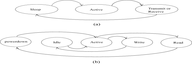
Figure 1: (a) Power state transition diagram of wireless radio module (b) Power state transition diagram of memory bank

To study the performance of power-aware buffering schemes, let’s discuss at length the power-mode transition pattern of radio and memory components. We assume that nodes use the radio-triggered power management, thus do not incur listening power consumption.

The power-mode of a multi-power radio component can be subsumed into 1) the sleep mode and 2) the active mode. A sleep-mode radio inhibits data transmission/reception. An active-mode radio permits data transmission/reception but incurs more power than when in sleep mode. To save power consumption, the radio is placed into sleep mode most of the time; it is only elevated to active mode (by a radio-triggered wakeup component) when data transmission/reception is needed. After completing data transmission/reception, the radio is put back to sleep mode. The sleep-active-transmit-sleep transition diagram in Figure 1(a) forms a typical power-aware radio working pattern.

A memory bank refers to the minimum size of a memory unit whose power mode can be independently altered [Hempstead2005]. Its power mode could be broadly classified into three categories: 1) the powerdown mode; 2) the idle mode; and 3) the active mode. A powerdown-mode memory bank means that the voltage supply to the memory bank is cut off, resulting in a sizable reduction in current leakage [Flautner2002;Tarjan2006]. The idle (sleep or drowsy) mode is the minimum power mode that preserves the stored information but inhibits writing and reading of data. An idle-mode or powerdown-mode memory bank must be reinstated to the active mode before a read/write operation can be performed. An active mode memory bank not only retains the stored information but also allows the data to be written/read. The power consumption in a powerdown-mode memory bank is negligibly small. An idle-mode memory bank consumes less power and has less functionality than an active-mode memory bank.

Figure 2: Evolution of powerdown-mode memory size (blue) and idle-mode memory size (red)

In an ideal power-saving data buffering scenario, the power-mode transition could be divided into 1) the write power-mode transition and 2) the read power-mode transition. A write power-mode transition is initiated by an interrupt of radio-triggered circuit. The sensor node first powers up the memory banks from the powerdown mode to the active mode, and then writes data into the memory banks. After completing a write operation, the involved memory banks are demoted to the idle mode to preserve power while retaining the stored information. The powerdown-active-write-idle power mode transition in Figure 1(b) forms a write operation cycle.

A read power-mode transition is initiated when a specified buffer size or interval threshold is reached. Thus, a read power-mode transition may comprise more than one write power-mode transition cycle, depending on the specified buffer size. It involves loading, transmitting and clearing up all the buffered data. To do so, it elevates the power mode of the buffered memory banks from idle mode to active mode. Once reading of data is completed, the corresponding memory banks are put back to powerdown mode. The idle-active-read-powerdown power mode transition in Figure 1(b) forms a read operation cycle, which is synchronized with the sleep-active-transmit-sleep power mode transition in the radio. In other words, data transmission in the radio is initiated immediately right after reading/loading buffered data from the memory banks.

The bottom graph in Figure 2 depicts the size of of arrival data (collected via sensors) as a function of time. The top graph shows the evolution of powerdown-mode memory size (total memory size minus stair height) and of idle-mode memory size (stair height). Observe that the powerdown-mode memory size shrinks as the arrival data are accumulated in idle-mode memory banks. The size of idle-mode memory banks grows in a stair-like fashion when it is less than the prescribed buffer size. Once it hits the prescribed buffer size and a transmission of buffered data is initiated. This forms a read power-mode transition cycle for memory banks, as well as a radio power-mode transition cycle. In practice, the duration of the read transition cycle may fluctuate widely: it could be very sensitive to the buffering policy, data arrival rate and data size distribution. In order to analyze the power-aware buffering issues, we begin with two buffering policies as follows:

Definition 1

A buffering policy is said to be stationary if its decision depends only on its current state and not on the time. A buffering policy is said to be deterministic if its decision is a deterministic function of the current state.

1. Fixed-size buffering scheme: data transmission is initiated immediately when a fixed (prescribed) buffer size is reached.

2. Fixed-interval buffering scheme: data transmission is commenced periodically with a fixed time interval.

There is a clear distinction between the well-known fixed-size and lesser-known fixed-interval buffering schemes: the threshold of the fixed-size buffering scheme depends on the size of the buffered data, and that of the fixed-interval one depends on a specified time interval. By definition 1, the fixed-size buffering scheme is stationary while the fixed-interval buffering scheme is deterministic. For notational convenience, we use the superscripts $FS$ and $FI$ to denote the fixed-size and fixed-interval buffering schemes throughout the paper. Before dwelling into a detailed derivation, we introduce relevant notions and essential prerequisites.

Definition 2

Let $x$ be a random variable following a probability distribution ${\cal F}$, i.e., $x\!\sim\!{\cal F}$, the skewness of $x$, denoted by $\gamma(x)$, is defined as

$$\gamma(x)=\dfrac{E[(x-\mu_{x})^{3}]}{(E[x-\mu_{x})^{2}])^{3/2}}=\dfrac{\mu_{3}}{\sigma_{x}^{3}}.$$ (1)

The coefficient of variation of $x$, denoted by $c_{v}(x)$, is defined as

$$c_{v}(x)=\dfrac{\sqrt{E[(x-\mu_{x})^{2}]}}{E[x]}=\dfrac{\sigma_{x}}{\mu_{x}},$$ (2)

where $E[]$ is the expected function and $\mu_{x}\!=\!E[x]$.

In probability theory, $\gamma(x)$ is the third standardized moment for measuring the degree of asymmetry. It can be further divided into positive ($\gamma(x)>0$) and negative skewness ($\gamma(x)<0$). The function $c_{v}(x)$ is a measure for the degree of dispersion.

Definition 3

An integer-valued random variable $\mathbf{n}$ is said to be a stopping time for the sequence $x_{1},x_{2},\cdots$ if the event $\{\mathbf{n}=n\}$ is independent of $x_{n+1},x_{n+2},\cdots$ for all $n=1,2,\cdots$.

Wald’s equation: Suppose $y_{1},y_{2}\cdots$ are iid random variable with finite expectation $E[y_{i}]\!=\!\mu_{y}$, and $\mathbf{n}$ is a stopping time for $y_{1},y_{2}\cdots$ such that $E[\mathbf{n}]<\infty$, then

$$E[\sum_{i=1}^{\mathbf{n}}y_{i}]=E[\mathbf{n}]E[y]\,=\,\mu_{y}E[\mathbf{n}]$$ (3)

The following theorem establishes the asymptotic behavior of stopping time variance w.r.t buffer size $b$.

Theorem 1

Let $\{x_{i}>0,i\geq 1\}$ be a random positive walk (increment) with mean of $\mu_{x}\!=\!E[x_{i}]\!>\!0$ and finite variance of $\sigma_{x}^{2}$. Let stopping time $\tau(b)=\min\{n\geq 1:\sum^{n}_{1}x_{i}>b\}$. When $b$ is sufficiently large, the stopping time variance $\sigma_{\tau_{b}}^{2}$ becomes

$$\sigma_{\tau_{b}}^{2}=\dfrac{b\sigma_{y}^{2}}{\mu_{y}^{3}}+k^{*}=\dfrac{bc_{v}^{2}(y)}{\mu_{y}}+k^{*}$$ (4)

where $k^{*}$ is expressed as

$$k^{*}=\dfrac{5c^{4}_{v}(y)}{4}+\dfrac{1}{12}-\dfrac{2c_{v}^{3}(x)\gamma(y)}{3},$$ (5)

where $c_{v}(y)$ denotes the coefficient of variation, and $\gamma(y)$ the skewness of $y$.

Proof of theorem 1 is given in the Appendix.

Theorem 1 states that in an asymptotic sense, the stopping time variance is linearly proportional to the buffer size $b$, with a proportionality constant of $c^{2}_{v}(y)/\mu_{y}$ and the intercept $k^{*}$ determined by both $c_{v}(x)$ and $\gamma(y)$. It means that $c^{2}_{v}(y)/\mu_{y}$ could play a central role in determining the stopping time variance. The magnitude of intercept ($k^{*}$) can be either mitigated by positive skewness or augmented by negative skewness. It is noteworthy that Theorem 1 is a special case of Lau’s theorem [Lai1977;Lai1979] under the positive random increment condition, which results in a substantial simplification. The following corollaries are special cases of Theorem 1 in which the random walk (increment) is assumed to be exponentially or Erlangly distributed.

Corollary 1

For a given buffer size $b$, the stopping time variance $\tau(b)$ for an exponential random walk with mean $1/\lambda_{e}$ is

$$\sigma^{2}_{\tau(b)}(exp)=\lambda_{e}b,$$ (6)

where $\sigma_{\tau(b)}(exp)$ refers to the stopping time variance w.r.t. an exponential random walk (increment).

Proof 2.2.

For an exponential random walk, by Definition 2 we get $c_{v}(y)=1,\gamma(y)=2$. Substituting $c_{v}(y)$ and $\gamma(y)$ into (4) leads to (6).

Corollary 2.3.

For a given buffer size $b$, the stopping time variance for an Erlang random walk with parameters $(\alpha,\!\lambda_{\alpha})$ is

$$\sigma^{2}_{\tau(b)}(erlang)=\frac{\lambda_{\alpha}b}{\alpha^{2}}+\frac{1}{12}(1-\frac{1}{\alpha^{2}}),$$ (7)

where $\alpha\!>\!1$ is the shape parameter (an integer), $\lambda_{\alpha}$ refers to the rate, and $\sigma_{\tau(b)}(erlang)$ refers to the stopping time variance w.r.t. an Erlang random walk (increment).

Proof 2.4.

By Definition 2, for an Erlang random walk, we obtain $c_{v}(y)\!=\!\frac{1}{\sqrt{\alpha}}$ and $\gamma(y)\!=\!\frac{2}{\sqrt{\alpha}}$. Substitution of $c_{v}(y)$ and $\gamma(y)$ into (4) yields (7).

Consider the differential stopping time variance between the exponential and the Erlang random walks by subtracting (6) with (7).

$$\sigma^{2}_{\tau(b)}(exp)-\sigma^{2}_{\tau(b)}(erlang)=b\lambda_{e}-\frac{\lambda_{\alpha}b}{\alpha^{2}}+\frac{1}{12}(1-\frac{1}{\alpha^{2}})$$ (8)

Notice that the mean increment size of exponential random walk is $\mu_{e}=1/\lambda_{e}$ and that of the Erlang walk is $\mu_{\alpha}=\frac{\alpha}{\lambda_{\alpha}}$. Letting $\mu_{\alpha}=\mu_{e}=\mu$, then (8) is reduced to

$$\sigma^{2}_{\tau(b)}(exp)-\sigma^{2}_{\tau(b)}(erlang)=(1-\frac{1}{\alpha})\left(\frac{b}{\mu}-\frac{1}{12}(1+\frac{1}{\alpha})\right),$$ (9)

then

$$\sigma^{2}_{\tau(b)}(exp)-\sigma^{2}_{\tau(b)}(erlang)\begin{cases}>0&\frac{b}{\mu}>\frac{1}{12}(1+\frac{1}{\alpha})\\ \leq 0&\frac{b}{\mu}\leq\frac{1}{12}(1+\frac{1}{\alpha}).\end{cases}$$ (10)

(10) means that with the same mean increment size, the stopping time under the exponential random walk (increment) has a wider variance than that under the Erlang walk as long as the condition $b>\mu/12$ is met.

Consider a hyper-exponential random walk (increment) as $\sum_{i=1}^{2}\!p_{i}\lambda_{i}\!\exp{(-\lambda_{i}x)}$ where $\sum_{i=1}^{2}\!p_{i}\!=\!1$ (letting $p_{1}=p,p_{2}=1-p$). The differential stopping time variance between the hyper-exponential and the exponential walks is $\sigma^{2}_{\tau(b)}(hp)\!-\!\sigma^{2}_{\tau(b)}(exp)$. Under the same mean increment, it becomes

$$\sigma^{2}_{\tau(b)}(hp)-\sigma^{2}_{\tau(b)}(exp)=\frac{b(c^{2}_{v}(y)-1)}{\mu}+k^{*},$$ (11)

where $k^{*}$ is explicitly given in (4). This implies that the differential stopping time variance is linearly proportional to the buffer size $b$, that is, $\sigma_{\tau(b)}^{2}(hp)-\sigma_{\tau(b)}^{2}(exp)\propto\frac{b}{\mu}(c^{2}_{v}(y)-1)>\!0$ when $b$ is sufficiently large. Namely, in an asymptotic sense, the hyperexponential random walk has a wider variance in the stopping time than the exponential walk under the same mean increment size condition.

Consider the fixed-size buffering scheme with a size of $b$. Define the stopping time, denoted by $\tau(b)$, to be a random variable that takes on values in $[0,\infty)$. One sees that $\tau(b)$ is a function of $b$ and the size distribution of the data $\{y_{i}>0:i\geq 0\}$:

$$\tau(b)=\min\{n:\sum_{i=1}^{n}y_{i}\geq b\},$$ (12)

where $\tau(b)$ is referred to as the first ladder epoch and $\sum_{i=1}^{\tau(b)}y_{i}$ is called the first epoch height [Lai1977;Lai1979;Feller1971].

Data Traffic
$\lambda$	Poisson data arrival rate
$\mu_{y}$	mean value of data size distribution
$b_{size}$	size of a memory bank
$\lambda\mu_{y}$	bandwidth
Radio Module
$e^{wu}_{w}$	energy for a radio wakeup
$e^{RX}_{w}$	energy for one-byte reception
$e^{TX}_{w}$	energy for one-byte transmission ($e^{RX}_{w}\approx e^{TX}_{w}$)
Memory Bank
$p^{idle}_{m}$	power of idle state of one memory bank
$e^{ena}_{m}$	energy to elevate from powerdown to active
$e^{dem}_{m}$	energy to demote from active to idle
$e^{r}_{m}$	energy of reading one byte
$e^{w}_{m}$	energy for writing one byte
$e^{resyn}_{m}$	$(e^{ena}_{m}+e^{dem}_{m})/2$

Table 1: Symbols and Meanings

One key step is to establish a relationship between the mean stopping time (the first ladder epoch) and the mean size of the data distribution. Assume that the sensor node has enough buffer capacity to accommodate first ladder height (overshoot) with respect to the buffer size $b$.

Theorem 2.5.

Let $\{y_{i}\!>\!0,\,i\!\geq\!0\}$ be the sequence of increment sizes with mean $\mu_{y}$, and $b$ be the buffer size, the mean stopping time $E[\tau(b)]\approx\frac{b}{\mu_{y}}$.

Proof 2.6.

By Wald’s equation in (3) we obtain the relation $\sum_{i=1}^{\tau(b)-1}y_{i}<b\leq\sum_{i=1}^{\tau(b)}y_{i}$. Taking expectation on both sides of this relation yields

$$E[\sum_{i=1}^{\tau(b)-1}y_{i}]<b\leq E[\sum_{i=1}^{\tau(b)}y_{i}]\Longrightarrow(E[\tau(b)]-1)\mu_{y}<b\leq E[\tau(b)]\mu_{y}.$$ (13)

Dividing both sides of (13) by $\mu_{y}$ completes the proof.

The preceding theorem asserts that the fixed-size buffering scheme with a buffer size of $b$ can hold $\frac{b}{\mu_{y}}$ data packets on average when the data size is randomly distributed with a mean of $\mu_{y}$, which is in line with our intuition.

For the sake of clarity, we summarize the power parameters in Table 1. The subscripts $m$ and $w$ denote the memory bank and radio module. $e^{ena}_{m}$ and $e^{dem}_{m}$ refer to the energy required to elevate a powerdown-mode memory bank to active mode, and to demote an active-mode memory bank to idle mode, $e^{resyn}_{m}$ is a resynchronization cost being equal to the mean value of $e^{ena}_{m}$ and $e^{dem}_{m}$, and $\lambda\mu_{y}$ the data volume per time unit, termed as bandwidth due to conceptual similarity. Since the duration of an active-mode memory bank is extremely short, thus the energy consumed in the active-mode could be reasonably ignored. Similarly, the energy consumed by the active-mode of a radio module is outweighed by $e^{TX}_{w},e^{RX}_{w}$, and hence is ignored.

3 Power-aware Buffering Schemes

3.1 Fixed-Size Buffering Scheme

In this subsection, we consider the fixed-size buffering scheme under randomly distributed data size with Poisson arrival. Assume that data size follows a certain probability distribution with a finite mean of $\mu_{y}$. Let $(x_{i},y_{i}),i\geq 0$ be a sequence of random vectors in which $\{x_{i},i\geq 0\}$ refers to a random variable denoting the interarrival times of Poisson arrival data and $\{y_{i},i\geq 0\}$ be a random variable representing the size of the arrival data. The random variables $x_{i}$ and $y_{i}$ are assumed to be mutually independent.

Theorem 3.7.

Let $\lambda$ be a Poisson arrival rate, $\mu_{y}$ be the mean data size, $b_{size}$ be the size of a memory bank, $e^{wu}_{w}$ be the per radio wakeup energy, and $p^{idle}_{m}$ be the idle-mode power consumption of a memory bank. Then the optimal buffer size $b^{*}$ for the fixed-size buffering scheme is

$$b^{*}=\sqrt{\frac{2b_{size}e^{wu}_{w}\lambda\mu_{y}}{p^{idle}_{m}}+\mu_{y}^{2}k^{*}}$$ (14)

where $k^{*}$ is given in (4).

Proof 3.8.

Consider a random vector sequence $(x_{i},y_{i})$, $i\geq 0$, where $\{x_{i},i\geq 0\}$ represents the arrival time instants (Poisson arrival) and $\{y_{i},i\geq 0\}$ is a sequence of received data sizes, with a mean $E[y_{i}]=\mu_{y}$ and a variance $\sigma^{2}_{y}$.

Define a renewal reward process [Ross1996] with the cycle length being equal to the time duration of stopping time $\tau(b)$ as follows:

$$L_{c}=\sum\limits_{i=0}\limits^{\tau(b)}x_{i+1}-x_{i},$$ (15)

where $L_{c}$ denotes the length of a renewal cycle, and $x_{i+1}\!-\!x_{i},i\geq 0$ is interarrival times. Letting $s_{k}=\sum^{k}_{i=1}x_{i}$. Thus the total energy $e^{FS}(b)$ over a renewal cycle is

$$e^{FS}(b) =e^{wu}_{w}+\dfrac{p^{idle}_{m}}{b_{size}}\sum_{i=1}^{\tau(b)}(s_{\tau(b)}-s_{i})y_{i}+\sum_{i=1}^{\tau(b)}(e^{TX}_{w}yi)+\sum_{i=1}^{\tau(b)}(e^{RX}_{w}y_{i}+e^{wu}_{w})$$ (16)

$$+\sum_{i=1}^{\tau(b)}(e^{w}_{m}+e^{r}_{m})y_{i}+2e^{resyn}_{m}$$

Let us return to explaining each term in (16). $\frac{p^{idle}_{m}}{b_{size}}\sum_{i=1}^{\tau(b)}(s_{\tau(b)}-s_{i})y_{i}$ denotes the accumulated idle-mode energy for the number of memory banks in a renewal cycle, and $\sum_{i=1}^{\tau(b)}e^{TX}_{w}y_{i}$ refers to the transmission energy, $\sum_{i=1}^{\tau(b)}(e^{w}_{m}+e^{r}_{m})y_{i}+2e^{resyn}_{m}$ is the total energy required to write/read data into/from the memory banks, plus the resynchronization energy, and $\sum_{i=1}^{\tau(b)}e^{RX}_{w}y_{i}+e^{wu}_{w}$ refers to the total energy for receiving data, plus the energy for radio wakeup for receiving data. The term $e^{wu}_{w}$ refers to per radio wakeup energy for data transmission. In other words, in each renewal cycle, the transmission radio wakeup occurs only once, while the reception radio wakeup occurs $\tau(b)$ times. Recall that we assume that nodes use the radio-triggered power management scheme, thereby the radio wake-up can be initiated without incurring listening energy. By Wald’s equation, we get

$$E[L_{c}]=E\left[\sum_{i=0}^{\tau(b)}x_{i+1}-x_{i}\right]=E[\tau(b)]E[x_{i+1}-x_{i}]=\frac{E[\tau(b)]}{\lambda}=\frac{b}{\lambda\mu_{y}}$$

Define $e^{FS}(t)$ to be the accumulated energy consumption at time $t$, where multiple renewal cycles may have occurred in the time period $[0,t]$. By the renewal reward theory [Ross1996], the long-run mean average energy consumption is

$$\overline{e^{FS}(b)}\stackrel{{\scriptstyle\text{\tiny def}}}{{=}}\lim_{t\rightarrow\infty}\dfrac{e^{FS}(t)}{t}=\dfrac{E[e^{FS}(b)]}{E[L_{c}]}=\dfrac{E[e^{FS}(b)]}{\frac{b}{\lambda\mu_{y}}},$$ (17)

where the unit of $\overline{e^{FS}(b)}$ is the watt (W), rather than the joule (J). Letting $e^{TX}_{w}=e^{RX}_{w}$. Taking expectation of the third term in (16) and applying Theorem 2.5 give

$$E\left[\sum\limits_{i=1}\limits^{\tau(b)}(2e^{TX}_{w}+e^{w}_{m}+e^{r}_{m})y_{i}+e^{wu}_{w}+2e^{resyn}_{m}\right]$$

$$=E[\tau(b)]E[(2e^{TX}_{w}+e^{w}_{m}+e^{r}_{m})y_{i}+e^{wu}_{w}+2e^{resyn}_{m}]$$

$$=\dfrac{b}{\mu_{y}}\left(\mu_{y}(2e^{TX}_{w}+e^{w}_{m}+e^{r}_{m})+e^{wu}_{w}+2e^{resyn}_{m}\right)$$ (18)

It follows from (4) and the assumption of independence of $y_{i}$ and $s_{i}=\sum_{j=1}^{i}x_{j}$, the expectation of the second term in (16) thus becomes

$$E\left[\sum\limits_{i=1}^{\tau(b)}(s_{\tau(b)}-s_{i})y_{i}\right] =\mu_{y}E\left[\sum\limits_{i=1}\limits^{\tau(b)}s_{\tau(b)}-s_{i}\right]=\dfrac{\mu_{y}(E[\tau^{2}(b)]-E[\tau(b)])}{2\lambda}$$ (19)

$$=\frac{\mu_{y}\left(E^{2}[\tau(b)]+\sigma^{2}_{\tau(b)}-E[\tau(b)]\right)}{2\lambda}=\dfrac{\dfrac{b^{2}}{\mu_{y}}+b(c^{2}_{v}(y)-1)+\mu_{y}k^{*}}{2\lambda},$$

where $k^{*}$ is given in (5). Substitution of (3.8)-(19) into (17) yields

$$\overline{e^{FS}(b)} =\dfrac{\lambda\mu_{y}e_{w}^{wu}+\frac{p_{m}^{idle}\mu_{y}^{2}k^{*}}{2b_{size}}}{b}+\lambda\left(\mu_{y}(2e^{TX}_{w}+e^{w}_{m}+e^{r}_{m})+e^{wu}_{w}+2e^{resyn}_{m}\right)$$

$$+\frac{p^{idle}_{m}\mu_{y}}{2b_{size}}(c^{2}_{v}(y)-1)+\frac{p_{m}^{idle}b}{2b_{size}}$$ (20)

Solving $\dfrac{\partial\overline{e^{FS}(b^{*})}}{\partial b^{*}}=0$ yields $b^{*}=\sqrt{\frac{2e^{wu}_{w}b_{size}\lambda\mu_{y}}{p^{idle}_{m}}+k^{*}\mu_{y}^{2}}$. To prove that $b^{*}$ is the optimal buffer size, it suffices to show that

$$\lim_{b\rightarrow b^{*}}\frac{\partial^{2}\overline{e^{FS}(b)}}{\partial b^{2}}=2\dfrac{e^{wu}_{w}\lambda\mu_{y}+\dfrac{p_{m}^{idle}k^{*}\mu_{y}^{2}}{2b_{size}}}{(b^{*})^{3}}>0.$$ (21)

The proof is thus completed.

The following corollary is a special case of Theorem 3.7.

Corollary 3.9.

When the size of received data is constant and identical to that of a memory bank, the optimal size of power-aware fixed-size buffering is expressed as

$$n^{*}=\sqrt{\dfrac{2\lambda e^{wu}_{w}}{p^{idle}_{m}}+\dfrac{1}{12}}\approx\sqrt{\dfrac{2\lambda e^{wu}_{w}}{p^{idle}_{m}}},$$ (22)

where $n^{*}$ in (22) refers to the number of memory banks used, hence the optimal buffer size is $b^{*}=n^{*}b_{size}$ ($b^{*}$ is a multiple of memory bank size $b_{size}$).

Proof 3.10.

It is almost trivial and therefore omitted.

Theorem 3.7 takes into account the impact of unevenly distributed data size, thereby generalizing the previous work [Ling2007] beyond the fixed-size data condition. It shows that the first two moments of data size distribution (mean and variance) alone are not sufficient to capture the dynamics of the power-aware fixed-size buffering. The term $\mu_{y}^{2}\,k^{*}$ in (14) represents the impact of varying-size data on the power-aware fixed-size buffering scheme, which is orthogonal to the data arrival rate $\lambda$. Such an impact can be quantitatively isolated in the form as:

$$\Delta_{v}b\!=\!\sqrt{\frac{2e^{wu}_{w}b_{size}\lambda\mu_{y}}{p^{idle}_{m}}+\mu_{y}^{2}k^{*}}\!-\!\sqrt{\frac{2e^{wu}_{w}b_{size}\lambda\mu_{y}}{p^{idle}_{m}}}$$ (23)

where $\Delta_{v}b$ refers to the purely size variation-induced impact on the fixed-size buffering scheme. Examination of $k^{*}$, at least in principle, can elucidate the respective roles of skewness and coefficient of variation in determining the optimal buffer size $b^{*}$. The effect of size variability could be either mitigated or augmented by the skewness in size distribution. A positive skewness alleviates the impact of size variability. In contrast, a negative skewness strengthens the impact of size variability. In this case, $k^{*}$ is positive and grows polynomially with $c_{v}(y)$, thereby ensuring $\Delta_{v}b>0$. This requires an additional buffer size be allocated in order to accommodate the variability in the data size distribution.

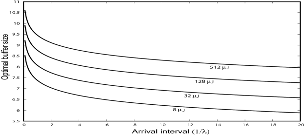
Figure 3: Optimal buffer size $b^{*}$ vs. $1/\lambda$: $\left[p_{m}^{idle}(0.409\mu W),b_{size}(256b),\mu_{y}(256b),e^{wu}_{w}(8\mu J,32\mu J,128\mu J,512\mu J)\right]$

Figure 3 plots the optimal buffer size ($b^{*}$) as a function of data arrival interval ($1/\lambda$) when the data size is exponentially distributed with a mean value of $256$ bytes. The curves are plotted in a semilog format: the $y$-axis refers to the optimal buffer size $b^{*}$ in a log scale and the $x$-axis refers to the mean data arrival time $1/\lambda$. It shows that an increase in per radio wakeup energy or in data arrival rate (decreasing data arrival interval) demands a large buffer size to reduce the amortized per radio wakeup cost. This observation agrees with intuition. Combining (14) and (3.8) gives the overall power consumption of the fixed-size buffering as follows:

$$\overline{e^{FS}(b^{*})}=\underbrace{\frac{p_{m}^{idle}b^{*}}{b_{size}}\!+\dfrac{p^{idle}_{m}\mu_{y}}{2b_{size}}\!(c_{v}^{2}(y)-1)+\lambda\left(2e^{resyn}_{m}+e^{wu}_{w}+\mu_{y}(e^{w}_{m}+e^{r}_{m})\right)}_{\mathrm{buffering}}+\underbrace{2\lambda\mu_{y}e^{TX}_{w}}_{\mathrm{trans/rec}}$$ (24)

(24) yields some interesting observations: the power consumption composition can be roughly divided into two pieces: 1) data transmission/reception power consumption is linearly proportional to bandwidth, i.e., $\lambda\mu_{y}$. 2) data buffering power consumption is quite complicated, hence resists a straightforward explanation: the buffering power consumption not only relies on data arrival rate $\lambda$ but also depends on the first three moments of the size distribution. (24) shows explicitly that the data buffering power consumption grows asymptotically in proportion to both $(c_{v}^{2}(y)-1)$ and the arrival rate $\lambda$, implying that the low-variance data size distribution ($c_{v}(y)\!<\!1$) consumes less power than the high-variance data size ($c_{v}(y)\!>\!1$).

3.2 Fixed-Interval Buffering Scheme

In this subsection we study the power-aware fixed-interval buffering scheme, which differs from its power-aware fixed-size counterpart. The following theorem gives a direct relation among the optimal time interval $T^{*}$, the power parameter of radio and memory bank, and data rate and the mean size of the data distribution.

Theorem 3.11.

Let $\lambda$ be a Poisson arrival rate, $\mu_{y}$ be the mean size of the data distribution, $e^{wu}_{w}$ be the per radio wakeup energy, and $p^{idle}_{m}$ be the idle state power consumption of a memory bank. Then, the optimal interval $T^{*}$ for the fixed-interval buffering scheme is:

$$T^{*} =\sqrt{\frac{2e^{wu}_{w}b_{size}}{p^{idle}_{m}\lambda\mu_{y}}}$$ (25)

Proof 3.12.

Let $T$ be the interval of the fixed-interval buffering scheme. The fixed-interval buffering is a special case of the renewal process in which the renewal cycle is constant. Hence the energy consumed in a renewal cycle is expressed as

$$e^{FI}(T) =e^{wu}_{w}+p^{idle}_{m}\sum_{i=1}^{n(T)}\dfrac{(T-s_{i})y_{i}}{b_{size}}+\sum_{i=1}^{n(T)}e^{TX}_{w}y_{i}+\sum_{i=1}^{n(T)}(e^{RX}_{w}y_{i}+e_{w}^{wu})$$ (26)

$$+\sum_{i=1}^{n(T)}(e^{w}_{m}+e^{r}_{m})y_{i}+2e^{resyn}_{m},$$

where $n(T)$ is a random variable denoting the number of data arrivals within the interval $T$, $y_{i}$ is the size of the ith arrived data, and the arrival time $s_{i}=\sum_{j=1}^{i}x_{j}-x_{j-1}$. The term $\sum_{i=1}^{n(T)}(e^{RX}_{w}y_{i}+e_{w}^{wu})$ refers to the total reception energy in the interval $T$, which involves the energy consumed in receiving the arrived data $\sum_{i=1}^{n(T)}e^{RX}_{w}y_{i}$, and the energy of radio wakeup for data reception $n(T)e_{w}^{wu}$. Notice that the radio-triggered power scheme does not incur listening power consumption. By the renewal reward theory, the long-run mean average energy consumption is

$$\overline{e^{FI}(T)}\stackrel{{\scriptstyle\text{\tiny def}}}{{=}}\lim_{t\rightarrow\infty}\dfrac{e^{FI}(t)}{t}=\dfrac{E[e^{FI}(T)]}{T}.$$ (27)

By Wald’s equation, the expectation of the second term in (26) is

$$\dfrac{p^{idle}_{m}}{b_{size}}E\left[\sum^{n(T)}_{i=1}(T-s_{i})I_{\{n(T)>0\}}y_{i}\right] =\dfrac{p^{idle}_{m}\mu_{y}}{b_{size}}\int^{T}_{0}(T-t)\lambda e^{-\lambda t}\left(\sum^{\infty}_{i=1}\dfrac{(\lambda t)^{i-1}}{(i-1)!}\right)\mathrm{d}t$$ (28)

$$=\dfrac{p^{idle}_{m}\mu_{y}\lambda}{b_{size}}\int^{T}_{0}(T-t)\mathrm{d}t=\dfrac{p^{idle}_{m}\mu_{y}\lambda T^{2}}{2b_{size}},$$

where $I_{\{n(T)>0\}}$ is the indicator function. Letting $e_{w}^{TX}\approx w_{w}^{RX}$, the expectation of the third-sixth terms in (26) are simplified as

$$E\left[\sum\limits_{i=1}\limits^{n(T)}y_{i}(2e^{TX}_{w}+e^{w}_{m}+e^{r}_{m})+2e^{resyn}_{m}+e^{wu}_{w}\right]$$ (29)

$$=E[n(T)]E[y_{i}(2e^{TX}_{w}+e^{w}_{m}+e^{r}_{m})+2e^{resyn}_{m}+e^{wu}_{w}]$$

$$=\lambda T(\mu_{y}\left(2e^{TX}_{w}+e^{w}_{m}+e^{r}_{m})+2e^{resyn}_{m}+w^{wu}_{w}\right).$$

Combining (27)-(29) gives

$$\overline{e^{FI}(T)}=\frac{E[\xi_{1}(T)]}{T}=\dfrac{e^{wu}_{w}}{T}+\dfrac{\lambda Tp^{idle}_{m}\mu_{y}}{2b_{size}}+\lambda\left(\mu_{y}(2e^{TX}_{w}+e^{w}_{m}+e^{r}_{m})+2e^{resyn}_{m}+e^{wu}_{w}\right)$$ (30)

Taking derivative of (30) w.r.t. $T$ gives $\dfrac{\partial\overline{e^{FI}(T)}}{\partial T}=-\dfrac{e^{wu}_{w}}{T^{2}}+\dfrac{p^{idle}_{m}\lambda\mu_{y}}{2b_{size}}$. Resolving $\frac{\partial\overline{e^{FI}(T^{*})}}{\partial T^{*}}=0$ leads to (25).

Examination of $T^{*}$ in (25) reveals the apparent variability immunity of the fixed-interval buffering scheme since $T^{*}$ only contains the first moment $\mu_{y}$ of the size distribution. Substituting (25) into (30) gives

$$\overline{e^{FI}(T^{*})} =\underbrace{\sqrt{\dfrac{2p^{idle}_{m}e^{wu}_{w}\lambda\mu_{y}}{b_{size}}}+\lambda(2e^{resyn}_{m}+e^{wu}_{w}+\mu_{y}(e^{w}_{m}+e^{r}_{m}))}_{\mathrm{buffering}}+\underbrace{\lambda 2\mu_{y}e^{TX}_{w}}_{\mathrm{trans/rec}}$$ (31)

In a similar fashion, the power consumption composition in (31) also can be divided into the data transmission/reception and buffering pieces. The data transmission/reception piece is linearly proportional to the bandwidth ($\lambda\mu_{y}$), while the data buffer one is proportional to the square root of the bandwidth $\sqrt{\lambda\mu_{y}}$. Although there is very little apparent relationship between the fixed-size and the fixed-interval buffering schemes, both buffering schemes essentially share the same transmission/reception component but differ markedly in their data buffering components: the data buffering component of the fixed-interval buffering scheme is a function of bandwidth. By contrast, that of the fixed-size buffering scheme is linked to the bandwidth and the first three moments of size distribution explicitly expressed in term $\mu_{y}^{2}k^{*}$.

Figure 4: Optimal buffer interval $T^{*}$ vs. $1/\lambda$: $\left[p_{m}^{idle}(0.409\mu W),b_{size}(256b),\mu_{y}(256b),e^{wu}_{w}(8\mu J,0.08mJ,0.8mJ,8mJ)\right]$

The curves in a semilog format in Figure 4 show that radio wakeup energy increase results in optimal time interval increase, while increasing idle-mode power consumption in a memory bank reduces the optimal buffer interval. This can be explained intuitively as follows: for a high per radio wakeup energy, a large data buffer (large optimal interval) can effectively reduce the amortized per radio wakeup energy, while a high sleep-mode power consumption would increase the power consumption of buffering, thereby reducing optimal buffer interval $T^{*}$.

Let us digress a little bit from the main derivation to examine the no-buffer scheme: a special case of the fixed-interval buffering scheme in which the sensor node transmits data immediately upon receipt of measured data. Mathematically, this corresponds to a case where the mean buffer interval $T\!=\!\frac{1}{\lambda}$. The following corollary deals with the no-buffer scheme.

Corollary 3.13.

The long-run mean average energy consumption of the no-buffer scheme, denoted by $\overline{e(nb)}$, is

$$\overline{e(nb)}=\lambda(2e^{wu}_{w}\!+\mu_{y}(2e^{TX}_{w}+e^{w}_{m}+e^{r}_{m})+2e^{resyn}_{m})$$ (32)

Proof 3.14.

Consider a renewal reward process with the cycle length ($\mathrm{L_{c}}$)being equal to the data arrival interval $T=1/\lambda$. Thus the energy consumed in this cycle is

$$e(nb)=e^{wu}_{w}+(2e^{TX}_{w}+e^{w}_{m}+e^{r}_{m})y_{i}+2e^{resyn}_{m}+e^{wu}_{w},$$ (33)

where $y_{i}$ is the size of ith arrived data. (33) is simply attained by removing the buffering factors (terms) in (28). Using the same argument in proving Theorem 3.11 we get $\overline{e(nb)}=\frac{E[e(nb)]}{\frac{1}{\lambda}}$ in (32) since $E[L_{c}]\!=\!\frac{1}{\lambda}$.

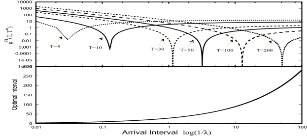
Figure 5: Top: $g^{FI}(T,T^{*})$ vs. arrival interval $\log(1/\lambda$). Bottom: $T^{*}$ vs. arrival interval $\log(1/\lambda)$: $\left[p_{m}^{idle}(0.409\mu W),e^{wu}_{m}(80\mu J),b_{size}(128b),\mu_{y}(64b)\right]$

Define a function $g^{FI}(T,T^{*})$ to quantify the differential gain of the optimal power-aware fixed-interval buffering over a power-oblivious buffering scheme.

$$g^{FI}(T,T^{*})=\overline{e^{FI}(T)}-\overline{e^{FI}(T^{*})}=\frac{e^{wu}_{w}}{T}+\dfrac{Tp^{idle}_{m}\lambda\mu_{y}}{2b_{size}}-\sqrt{\frac{2p^{idle}_{m}e^{wu}_{w}\lambda\mu_{y}}{b_{size}}},$$ (34)

where $T^{*}$ is the optimal interval and $T$ is chosen arbitrarily.

Results of $g^{FI}(T,T^{*})$ are plotted in Figure 5. The main trend is that the optimal buffer interval $T^{*}$ grows as the square root of $\frac{1}{\lambda}$ (see bottom graph), and that a dip in each curve occurs when arbitrarily chosen $T$ happens to be in the vicinity of $T^{*}$. The differential gain $g^{FI}(T,T^{*})$ arises sharply when $T$ deviates from the optimal buffer interval $T^{*}$. This implies that a blind selection of buffer interval $T$ is very likely to incur an excessive energy consumption.

4 Performance Comparison

In this section we attempt to answer two fundamental questions: 1) how much power saving via power-aware buffering can be achieved in comparison to the no-buffer scheme ? 2) the fixed-size buffering or its fixed-interval counterpart, which one performs better ?

4.1 Comparison between the no-buffer scheme and power-aware buffering schemes

It is evident that the fixed-interval buffering always outperforms the no-buffer scheme as the latter is a special case of the former. Below we compare the no-buffer scheme with the fixed-size buffer one.

The differential power consumption between the no-buffer and optimal fixed-size buffering schemes is expressed as

$$\overline{e(nb)}-\overline{e^{FS}(b^{*})}=\lambda e^{wu}_{w}-\frac{p_{m}^{idle}}{b_{size}}\left(b^{*}+\dfrac{\mu_{y}(c^{2}_{v}(y)-1)}{2}\right)>0$$ (35)

(35) does in fact constitute an incentive condition under which the optimal fixed-size buffering scheme outperforms the no-buffer scheme in power conservation. It shows that increasing variability $c_{v}(y)$ in effect erodes the gain brought out by the power-aware fixed-size buffering scheme, hence shrinks the incentive area. A positive skewness in size distribution can neutralize, to some extent, the size variability-induced impact. While in general this incentive condition could be profoundly affected by various intertwined and correlated factors, we explicitly derive closed-form expressions under some restricted scenarios:

1) Exponential data size distribution $y$ with a mean of $\mu_{y}$. Under this condition, $k^{*}$ is reduced to zero according to (4), the incentive condition thus becomes

$$\overline{e(nb)}-\overline{e^{FS}(b^{*})}=\lambda e^{wu}_{w}-\frac{p_{m}^{idle}b^{*}}{b_{size}}=\lambda e^{wu}_{w}-\sqrt{\frac{2\lambda p_{m}^{idle}e_{w}^{wu}\mu_{y}}{b_{size}}}>0$$ (36)

It is obvious that (36) holds as long as $\lambda e^{wu}_{w}\!>\!\frac{2p^{idle}_{m}\mu_{y}}{b_{s}ize}$ is met. This incentive condition can be rewritten in a structurally meaningful form that emphasizes the distinction between hardware parameters and operational requirement as follow

$$\dfrac{e^{wu}_{w}}{\frac{p^{idle}_{m}}{b_{size}}}>\frac{2\mu_{y}}{\lambda}.$$ (37)

Using byte-second as a quantifiable unit, the left-hand side of (37) is related to hardware power parameters: the ratio of radio wakeup energy to the per-byte idle-mode power consumption of a memory bank. The right-hand side, on the other hand, is related to the operational requirement: the ratio of the mean data size to the data arrival rate. For given power parameters and $\mu_{y}$, there exists a critical value for $\lambda_{c}\!=\!\frac{2\mu_{y}p^{idle}_{m}}{b_{size}e^{wu}_{w}}$. When $\lambda>\lambda_{c}$, the fixed-size buffering scheme is preferred. Otherwise, the no-buffer scheme is preferred. A high ratio of the per radio wakeup energy to the per-byte idle-mode memory power consumption favors a large buffer size. On the other hand, the benefit of data buffering is diminished as $\frac{\mu_{y}}{\lambda}$ increases.

2) Erlang size distribution $y$ with parameters $(\alpha,\lambda_{\alpha})$. This corresponds to the case in which $c_{v}(y)=\frac{1}{\sqrt{\alpha}},\gamma(y)=\frac{2}{\sqrt{\alpha}},\mu_{y}=\dfrac{\alpha}{\lambda_{\alpha}},\sigma_{y}=\dfrac{\sqrt{\alpha}}{\lambda_{\alpha}}$, then $k^{*}=\!\frac{1}{12}(1-\frac{1}{\alpha^{2}})$. The incentive condition is thus expressed as

$$\overline{e(nb)}-\overline{e^{FS}(b^{*})}=\lambda e^{wu}_{w}-\frac{p_{m}^{idle}}{b_{size}}\left(b^{*}-\frac{\mu_{y}}{2}(1-\frac{1}{\alpha})\right)>0$$ (38)

where

$$b^{*}=\sqrt{\frac{2\lambda b_{size}e_{w}^{wu}\mu_{y}}{p^{idle}_{m}}+\frac{\mu_{y}^{2}}{12}(1-\frac{1}{\alpha^{2}})}$$ (39)

(39) shows that, as compared with an exponential size distribution ($\alpha=1$), an additional buffer size needs to be allocated when the shape parameter $\alpha>1$. To study the impact of data arrival rate $\lambda$, we define $f(\lambda)=\overline{e(nb)}\!-\!\overline{e^{FS}(b^{*})}$. Differentiating $f(\lambda)$ and solving $f^{\prime}(\lambda^{*})=0$ gives

$$\lambda^{*}=\frac{\mu_{y}p^{idle}_{m}}{24b_{size}e^{wu}_{w}}\left(11+\frac{1}{\alpha^{2}}\right)$$ (40)

Observe that $f(\lambda)$ has a global minimum point at $\lambda^{*}$ since $f^{\prime\prime}(\lambda^{*})>0$. This implies that $f(\lambda^{*})<f(\lambda),\lambda\in{\cal R}^{+}$ and $\lambda\not=\lambda^{*}$. Substituting (40) into (38) gives

$$f(\lambda^{*})=-\frac{\mu_{y}p^{idle}_{m}}{24b_{size}}\left(1+\frac{12}{\alpha}-\frac{1}{\alpha^{2}}\right)<0,\ \ \alpha\geq 1$$ (41)

Since $f(0)=\frac{p^{idle}_{m}\mu_{y}}{2b_{size}}\left(1-\frac{1}{\alpha}-\frac{1}{\sqrt{3}}\sqrt{1-\frac{1}{\alpha^{2}}}\right)\leq 0,\alpha\geq 1$, and $f(\lambda)\rightarrow e^{wu}_{w}\lambda>0$ when $\lambda$ is sufficiently large, one concludes that there exists a critical data rate $\lambda_{c}>\lambda^{*}$ such that the no-buffer scheme outperforms the fixed-size buffering scheme when $\lambda\leq\lambda_{c}$ and the fixed-size buffering scheme is preferred when $\lambda>\lambda_{c}$. Figure 6 plots $f(\lambda)$ as a function of $1/\lambda$ with different shape parameters in a semilog format. Figure 6 illustrates that increasing shape parameter $\alpha$ (less variation) results in a decreased critical data rate $\lambda_{c}$ (increasing $T_{c}=1/\lambda_{c}$), indicating that the smaller the data size variation, the larger the incentive region. It is worth noting that there exists an inherent tradeoff between buffering and responsiveness: the no-buffer scheme achieves real-time responsiveness at the expense of power consumption, while the power-aware buffering to some extent can save power consumption, but at the price of reduced responsiveness.

Figure 6: Incentive area vs. arrival interval: $\left[p_{m}^{idle}(0.409\mu W),b_{size}(256b),e^{wu}_{m}(80\mu J),\mu_{y}(64b)\right]$

4.2 Comparison between Fixed-size and Fixed-interval Buffering Schemes

One question arises naturally: which buffering scheme is more power efficient? the power-aware fixed-size scheme or the power-aware fixed-interval one. While in general there is no simple answer to this question, there is a definite answer under some special circumstances. We begin with an easy lemma as below.

Lemma 4.15.

Let $f(x)\!=\!\sqrt{ax}-\!\sqrt{ax+b}\!+\!c,x\geq 0$, where $a,b$, and $c$ are positive, and $\sqrt{b}<c$. Then $f(x)\!>\!0$ for $x\!\geq\!0$.

Proof 4.16.

Take derivation of $f(x)$, we obtain

$$f^{\prime}(x)=\dfrac{a(\sqrt{ax+b}-\sqrt{ax})}{2\sqrt{ax(ax+b)}}>0,x>0$$ (42)

This means that $f(x)$ is monotonically increasing for $x\!\geq\!0$. Then $f(0)\!=\!\min\limits_{x\in(0,\infty)}\!f(x)$. It can be inferred that $f(x)>f(0)>0$ for $x\geq 0$ since $f(0)\!=\!-\sqrt{b}+c>0$.

Theorem 4.17.

The power-aware fixed-size buffering scheme is more power-efficient than the fixed-interval counterpart when the data size is constant, while both the buffering schemes perform equally well when the data size is exponentially distributed.

Proof 4.18.

Define $g(T^{*},b^{*})$ to denote the power consumption differential between the fixed-interval and fixed-size buffering schemes as follows

$$g(T^{*},b^{*}) =\overline{e^{FI}(T^{*})}-\overline{e^{FS}(b^{*})}=\sqrt{\dfrac{2\mu_{y}\lambda p^{idle}_{m}e^{wu}_{w}}{b_{size}}}-\frac{p_{m}^{idle}}{b_{size}}\left(b^{*}+\dfrac{\mu_{y}(c^{2}_{v}(y)-1)}{2}\right)$$ (43)

(I) Constant data size: Since $\sigma_{y}\!=\!0$ and $k^{*}\!=\!1/12$, thus (43) becomes

$$g(T^{*},b^{*})=\sqrt{\dfrac{2\mu_{y}\lambda p^{idle}_{m}e^{wu}_{w}}{b_{size}}}-\sqrt{\dfrac{2\mu_{y}\lambda p^{idle}_{m}e^{wu}_{w}}{b_{size}}+\dfrac{(\mu_{y}p^{idle}_{m})^{2}}{12b^{2}_{size}}}+\dfrac{p^{idle}_{m}\mu_{y}}{2b_{size}}$$ (44)

Let $a\!=\!\frac{2\mu_{y}p^{idle}_{m}e^{wu}_{w}}{b_{size}},\,b=\!\frac{(\mu_{y}p^{idle}_{m})^{2}}{12b_{size}^{2}},\,c\!=\!\frac{p^{idle}_{m}\mu_{y}}{2b_{size}}$. Based on Lemma 4.15, we have $g(T^{*},b^{*})>0$, i.e., $\overline{e^{FI}(T^{*})}>\overline{e^{FS}(b^{*})}$.

(II) Exponential size distribution: Since $\sigma_{y}\!=\!\mu_{y},c_{v}(y)\!=\!1,\gamma(y)\!=\!2$, thus $k^{*}\!=\!0$, (43) becomes

$$g(T^{*},b^{*})\!=\!\sqrt{\dfrac{2\mu_{y}\lambda p^{idle}_{m}e^{wu}_{w}}{b_{size}}}\!-\!\sqrt{\dfrac{2\mu_{y}\lambda p^{idle}_{m}e^{wu}_{w}}{b_{size}}}=0.$$ (45)

Combining (I)-(II) completes the proof.

Consider a hyper-exponential size distribution: $f_{h}(y)=\sum_{i=1}^{2}\frac{1}{\mu_{i}}p_{i}\exp{(-y/\mu_{i})}$ and $\sum_{i=1}^{2}p_{i}\!=\!1$. Letting $p_{1}\!=\!p,p_{2}\!=\!1-p$. Since there is no closed-form expression for $g(T^{*},b^{*})$, thus a numerical method is used to compute different values for $c_{v}(y)$ and $\gamma(y)$. This is achieved by varying the value of $p$ while maintaining $\mu_{y}$ constant. Figure 7 presents $g(T^{*},b^{*})$ as a function of $\frac{1}{\lambda}$ with different $c_{v}(y)$ and $\gamma(y)$. It shows that $c_{v}(y)$ has a substantial impact on $g(T^{*},b^{*})$, whereas $\gamma(y)$ plays a marginal role. For example, when $c_{v}(y)\!=\!1.72$ and $\gamma(y)=2.72$, $g(T^{*},b^{*})\!=\!\overline{e^{FI}(T^{*})}\!-\!\overline{e^{FS}(b^{*})}\!<\!0$.

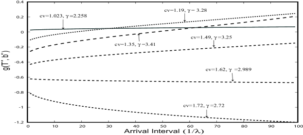
Figure 7: $g(T^{*},b^{*})$ vs. $1/\lambda$: $\left[p_{m}^{idle}(0.409\mu W),e^{wu}_{m}(80\mu J),b_{size}(256b)\right]$

Combining the above analysis and numerical calculation leads to the conclusion that the size variation-induced effect is a non-negligible role in determining the relative advantages of the fixed-interval and fixed-size buffering schemes: when the size distribution is of low-variance, the fixed-size buffering scheme outperforms the fixed-interval counterpart. When the size distribution is of high-variance, the fixed-interval buffering scheme is more energy-efficient than the fixed-size one. Between these two extremes in size variability, the relative power efficiency of these two buffering schemes depends on data arrival rate $\lambda$.

To illustrate the efficacy of the power-aware fixed-size buffering scheme over a power-oblivious one, we define a function $g^{FS}(b,b^{*})$ as follows

$$g^{FS}(b,b^{*})=\overline{e^{FS}(b)}-\overline{e^{FS}(b^{*})}=(b^{*}-b)\left(\frac{\lambda e^{wu}_{w}\mu_{y}+\dfrac{p^{idle}_{m}\mu_{y}^{2}k^{*}}{2b_{size}}}{b\cdot b^{*}}-\frac{p^{idle}_{m}}{2b_{size}}\right),$$ (46)

where $b^{*}$ denotes the optimal buffer size (see (14)), and $b$ is arbitrarily chosen ($b\in{\cal R}$ and $b\not=b^{*}$). In practical terms, the amount of power consumed in the idle-mode memory banks is quantized into discrete levels as $p_{m}^{idle}\!\left\lceil\frac{b}{b_{size}}\right\rceil$, where $\lceil\rceil$ is the ceiling function. This implies that only certain discrete power states are allowed. For example, if $b_{size}\!=\!128$, then two memory banks will be used when the buffer size $b$ falls within the range of $[128,255\,]$.

To visualize this quantization impact, we examine the function $g^{FS}(b,b^{*})$ when $k^{*}=0$ (an exponential size distribution). Figures 8-9 plot $g^{FS}(b,b^{*})$ as a function of $1/\lambda$ under different values of $\mu$ (mean data size). The y-axis in the top graph in Figure 8 represents $g^{FS}(256,b^{*})$ in the unit of ($\mu W$). The y-axis in the bottom graph in Figure 8 denotes the optimal buffer size $b^{*}$ in a multiple of $b_{size}$. The x-axis refers to the mean arrival interval $1/\lambda$ in a $\log$ scale.

With increases in $\frac{1}{\lambda}$, the optimal buffer size $b^{*}$ decreases. The curve of $g^{FS}(256,b^{*})$ gradually declines as $\frac{1}{\lambda}$ increases, as shown in Figure 8. In contrast, in Figure 9 with increases in $\frac{1}{\lambda}$, the differential gain $g^{FS}(1280,b^{*})$ initially monotonically decreases and then increases after reaching the lowest point at which the buffer size $b$ is optimal at $10b_{size}=1280$. Observe that the memory-bank-size quantized effect produces a stair-like relation between the amount of power consumed and $\frac{1}{\lambda}$. For example, the optimal buffer size is $6b_{size}$ when $\frac{1}{\lambda}\in[5.435,7.825)$. The larger the arrival interval $\frac{1}{\lambda}$, the more pronounced (a wider stair space) the quantized effect.

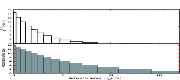
Figure 8: Top: $g^{FS}(256,b^{*})$ vs arrival rate $\log(1/\lambda)$ Bottom: optimal buffer size $b^{*}$ vs. $\log(1/\lambda)$ $\left[b_{size}(128b),\mu_{y}(64b),e^{wu}_{w}(80\mu J),p^{idle}_{m}=0.409\mu W\right]$

Figure 9: Top: $g^{FS}(1280,b^{*})$ vs. $\log(1/\lambda)$. Bottom: optimal buffer size $b^{*}$ vs. $\log(1/\lambda)$. $\left[b_{size}(128b),\mu_{y}(64b),e^{wu}_{w}(80\mu J),p^{idle}_{m}(0.409\mu W)\right]$

Figure 10: Top: $g^{FS}(256,b^{*})$ vs. $\log(1/\lambda)$) Bottom: optimal buffer size $b^{*}$ vs. $\log(1/\lambda)$ $\left[b_{size}(128b),\mu_{y}(64b),e^{wu}_{w}(80\mu J),p^{idle}_{m}(0.409\mu W),c_{v}(y)(1.723),\gamma(y)(2.718)\right]$

Figure 11: Top: $g^{FS}(1280,b^{*})$ vs. $\log(1/\lambda)$ Bottom: optimal buffer size $b^{*}$ vs. $\log(1/\lambda)$ $\left[b_{size}(128b),\mu_{y}(64b),e^{wu}_{w}(80\mu J),p^{idle}_{m}(0.409\mu W),c_{v}(y)(1.723),\gamma(y)(2.718)\right]$

To evaluate the size variation-induced effects, we calculated $g^{FS}(b,b^{*})$ under a hyperexponentially distributed data size in which $c_{v}(y)=1.732$ and $\gamma(y)=2.718$ and plot both $g^{FS}(256,b^{*})$ and $g^{FS}(1280,b^{*})$ as a function of $\frac{1}{\lambda}$ in Figures 10-11, respectively. In comparison to the absence of size variation as shown in Figures 8-9, the size variation effect becomes inconsequential when $\lambda$ is high, but has a substantial impact when $\lambda$ is low (see Figure 12).

Figure 12: Top: Optimal buffer size $b^{*}$ vs. $\log(\frac{1}{\lambda}):(c_{v}(y)(1.723),\gamma(y)(2.718))$. Bottom: Optimal buffer size $b^{*}$ vs. $\log(\frac{1}{\lambda}):(c_{v}(y)(0))$ $[b_{size}(128b),\mu_{y}(64b),e^{wu}_{w}[80\mu J),p^{idle}_{m}(0.409\mu W)]$

This phenomenon can be explained by reference to (23). $\Delta_{v}b$ in (23) shows that the size variation effect is proportional to the term $\mu_{y}^{2}k^{*}$. Hence the relative effect of size variation on the optimal buffer size $b^{*}$ can be expressed as

$$\frac{\Delta_{v}b}{\sqrt{\frac{2\lambda e^{wu}wb_{size}\mu_{y}}{p^{idle}_{m}}}}=\sqrt{1+\frac{\mu_{y}p^{idle}_{m}k^{*}}{2\lambda e^{wu}_{m}b_{size}}}-1$$ (47)

(47) indicates that for a given size distribution (given $c_{v}(y)$ and $\gamma(y)$, thereby $k^{*}$), the size variability effect becomes prominent for low duty-cycle sensor nodes as (47) increases with decreasing $\lambda$ (low duty cycle).

5 Effect of power-aware buffering schemes on life span

In this section we will use a concrete example to quantify the benefits of power-aware schemes in terms of the lifespan extension.

$e^{wu}_{w}$	$p^{idle}_{m}$	$e^{TX}_{w}$	$e^{r}_{m}+e^{w}_{m}$	$e^{resyn}_{m}$
$80~{}\mu J$	$0.409~{}\mu W$	$8.976~{}\mu J/byte$	$36\cdot 10^{-3}\mu J/byte$	$0.912~{}\mu J$

Table 2: Power parameters of radio and memory bank

Power parameters in Table 2 are either directly obtained or indirectly derived from the literature. In CC2420-802.15.4 radio specification [CC2420], the transmission power is $-25\,dBm$ with a data rate of $250$ kbps, and the current draw is $8.5\,mA\,(3.3V)$. The $250$ kbps is the optimal rate in an ideal environment, which may not make any practical sense. In practical terms, the rate is assumed to be $25$ kbps. Consequently, the one-byte transmission energy is calculated as $e^{TX}_{w}=\frac{8.5\times 3.3\times 8}{25}=8.976\mu J/byte$. The power consumption for an idle-mode SRAM memory bank is $p^{idle}_{m}=0.409\mu W$ [Hempstead2005]. Due to unavailability of actual power data of SRAM bank in the literature, the $e^{r}_{m},e^{w}_{m},e^{resyn}_{m}$ are approximated by using Rambus DRAM power data. A read or write operation on Rambus DRAM takes $60ns$ and consumes $300mW$, i.e., $e^{r}_{m}=e^{w}_{m}=18\cdot 10^{-3}\mu J/byte$. A transition from the powerdown mode of a Rambus DRAM to the active mode consumes $152mW$ and takes $6000ns$ [Fan2001]. Thus a resynchronization energy is $e^{resyn}_{m}=0.912\,\mu J$. A radio wakeup energy is assumed to be $e^{wu}_{w}=80\,\mu J$ as it is not found in literature. Let the supply voltage be $3.3\,V$, and the lifespan of two AA batteries be $2700\,mAh$ [Levis2005].

Consider a scenario with a Poisson arrival and constant data size (implying $k^{*}=1/12$). Letting $y_{i}=\mu_{y}=b_{size}=128b$. Based on Table 2, the comparison results between the optimal fixed-size buffering, optimal fixed-interval buffering, and an power-oblivious buffering with buffer size of $256$ are tabulated in Table 3.

With $\lambda=0.5$, by (14), the optimal buffer size is calculated as $b^{*}=1790.54$(b), thus the number of memory banks involved is $\lceil\frac{b^{*}}{b_{size}}\rceil\!=14$. By (24), we obtain $\overline{e^{FS}(b^{*})}=1197.660858\,\mu W$. The amount of current draw is $\frac{1197.660858}{3.3}=362.927533\mu A$, and the lifespan is $\frac{3.3*2700000}{1197.660858*24*365}=0.849258$(yr). Similarly, the power consumption of the power-oblivous and optimal fixed-interval schemes are calculated as $\overline{e^{FS}(256)}=1212.357021\mu W$ and $\overline{e^{FI}(T^{*})}=1197.864140\,\mu W$. This implies that the power-aware fixed-size scheme outlives the power-oblivious one by $3.75761$ days and outlives the optimal fixed-interval one by $1.262509$ hours.

Table 3 shows that the role of the power-aware buffering becomes more prominent when the node operates at a low duty cyle. For example, with $\lambda=1$, the optimal fixed-size buffer scheme outlives the power-oblivious one by $2.069278$ days, when $\lambda=0.1$, the optimal fixed-size buffer scheme outlives the power-oblivious one by $11.797951$ days. A side-by-side comparison in Table 3 suggests that the fixed-size buffering scheme performs slightly better than the fixed-interval counterpart. However, this marginal advantage will be disappeared in the presence of data-size variations.

$\lambda$	$\overline{e^{FS}(b^{*})}$	lifespan	$\overline{e^{FI}(T^{*})}$	lifespan	$\overline{e^{FS}(256)}$	lifespan
$(1/s)$	$(\mu W)$	(yr)	$(\mu W)$	(yr)	$(\mu W)$	(yr)
$1$	$2392.1739$	$0.4252$	$2392.3775$	$0.4252$	$2424.5010$	$0.4195$
$0.9$	$2153.3299$	$0.4723$	$2153.5336$	$0.4723$	$2182.0722$	$0.4661$
$0.8$	$1914.4623$	$0.5313$	$1914.6659$	$0.5312$	$1939.6434$	$0.5244$
$0.7$	$1675.5663$	$0.6070$	$1675.7698$	$0.6069$	$1697.2146$	$0.5993$
$0.6$	$1436.6355$	$0.7080$	$1436.8389$	$0.7079$	$1454.7858$	$0.6992$
$0.5$	$1197.6609$	$0.8493$	$1197.8641$	$0.8491$	$1212.3570$	$0.8390$
$0.4$	$958.6283$	$1.0610$	$958.8314$	$1.0608$	$969.9282$	$1.0487$
$0.3$	$719.5143$	$1.4136$	$719.7172$	$1.4132$	$727.4994$	$1.3981$
$0.2$	$480.2728$	$2.1178$	$480.4753$	$2.1169$	$485.0706$	$2.0969$
$0.1$	$240.7851$	$4.2242$	$240.9869$	$4.2207$	$242.6418$	$4.1919$

Table 3: Performance comparison

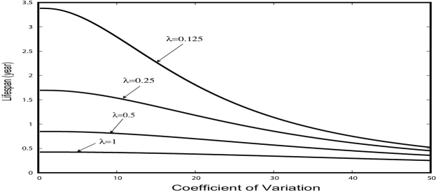
Figure 13: Life span vs $c_{v}(y)$ $[b_{size}(128b),\mu_{y}(128b),e^{wu}_{w}(80\mu J),p^{idle}_{m}(0.409\mu W)]$

To see the size variation effect on the fixed-size buffering scheme, we consider a hypothetical symmetrical size distribution ($\gamma(y)=0$). Thus the optimal buffer size $b^{*}$ is expressed as

$$b^{*}=\sqrt{\frac{2\lambda e^{wu}_{m}\mu_{y}b_{size}}{p^{idle}_{m}}+\mu_{y}^{2}(\frac{5c^{4}_{v}(y)}{4}+\frac{1}{12})}$$ (48)

Based on (24) and Table 2, Figure 13 plots the lifespan as a function of $c_{v}(y)$ under different data arrival rates ($\lambda$). One can see a monotonic decline in the lifespan with increasing $c_{v}(y)$. This trend indicates that for the fixed-size buffering scheme, high data size variation has a detrimental effect that further depletes battery. By contrast, the fixed-interval buffering scheme has an obvious advantage of being eminently immune to data size variation: its power consumption is only associated to mean data size $\mu_{y}$, and is independent of data size variance. To illustrate, under two power parameter settings, the lifespan, optimal buffer interval $T^{*}$, and the power consumption under different rates are given in Table 4.

$\lambda(1/s)$	$T^{*}(s)$	$\overline{e^{FI}(T^{*})}(\mu W)$	lifespan (yr)	$T^{*}$ (s)	$\overline{e^{FI}(T^{*})}(\mu W)$	lifespan (yr)
$1$	$19.79$	$2392.38$	$0.425$	$12.65$	$3230.78$	$0.315$
$0.5$	$13.99$	$4780.02$	$0.213$	$8.94$	$6387.46$	$0.159$
$0.25$	$9.89$	$9553.33$	$0.107$	$6.32$	$12670.13$	$0.08$
$0.125$	$6.99$	$19097.18$	$0.053$	$4.47$	$25192.07$	$0.04$
$0.0625$	$4.94$	$38180.97$	$0.027$	$3.16$	$50174.57$	$0.02$
power	$e^{wu}_{w}(80\,\mu J)$, $p^{idle}_{m}(0.409\,\mu W)$			$e^{wu}_{w}(800\,\mu J)$, $p^{idle}_{m}(10\,\mu W)$
parameters	$e^{TX}_{w}(8.976\,\mu J/byte)$			$e^{TX}_{w}(8.976\,\mu J/byte)$
	$b_{size}(128b),\mu_{y}(128b),e^{r}_{m}+e^{w}_{m}(36\cdot 10^{-3}\mu J/byte)$

Table 4: Lifespan under data arrival rates for fixed-interval buffering scheme

For environmental monitoring, a sensor-based network forms a data collection tree. Each node gathers local information, and forwards the data from its child nodes to its routing parent (see Figure 14). The sink node then collates the received information into global environmental data. Below we establish an energy consumption relationship between a routing parent node and its child nodes in the context of fixed-interval buffering scheme.

Figure 14: Data collection tree: bandwidth conservation between parent and child nodes

Theorem 5.19.

Suppose a parent node has $k$ child nodes in a static data collection tree. Let the ith child have Poisson arrival with a rate of $\lambda_{i}$ and a mean size of $\mu_{i}$. If the parent and child nodes adopt the fixed-interval buffering scheme, then the optimal buffer interval $T_{p}^{*}$ for the parent node is

$$T^{*}_{p}=\sqrt{\frac{2e^{wu}_{w}b_{size}}{p^{idle}_{m}\sum\limits_{i=1}^{k}\lambda_{i}\mu_{i}}}.$$ (49)

Proof 5.20.

It follows from (25) that for the ith child node, its optimal interval is $T_{i}=\sqrt{\frac{2e^{wu}_{w}b_{size}}{p^{idle}_{m}\lambda_{i}\mu_{i}}}$. This means that successive transmission from the ith node to its parent node is equally spaced by an interval $T_{i}$, with the mean size of $\lambda_{i}T_{i}\mu_{i}$. Assume that each node has the radio-triggered wakeup capability, thereby incurring no listening power consumption.

Let $T$ be the length of a renewal cycle of the parent node. Each child node independently transmits the buffered data at the rate of $1/T_{i}$. With respect to the ith child, the corresponding energy consumed by the parent node, denoted by $e^{FI}(T)(i)$, can be decomposed into three pieces:

1) The energy for data buffering (idle-mode) at the parent node, denoted by $e^{FI}_{b}(T)(i)$, is bounded as:

$$\sum_{k=1}^{\lfloor\frac{T}{T_{i}}\rfloor}\dfrac{p_{m}^{idle}(T-kT_{i})y_{i}(k)}{b_{size}}\leq e^{FI}_{b}(T)\leq\sum_{k=0}^{\lfloor\frac{T}{T_{i}}\rfloor}\dfrac{p_{m}^{idle}(T-kT_{i})y_{i}(k)}{b_{size}},$$ (50)

where $y_{i}(k)$ is the size of kth data sent by the i child node, and $E[y_{i}(k)]=\lambda_{i}T_{i}\mu_{i}$.

$$\sum_{k=1}^{\lfloor\frac{T}{T_{i}}\rfloor}\dfrac{p_{m}^{idle}(T-kT_{i})\lambda_{i}T_{i}\mu_{i}}{b_{size}}\leq E[e^{FI}_{b}(T)]\leq\sum_{k=0}^{\lfloor\frac{T}{T_{i}}\rfloor}\dfrac{p_{m}^{idle}(T-kT_{i})\lambda_{i}T_{i}\mu_{i}}{b_{size}}.$$ (51)

This yields $E[e^{FI}_{b}(T)(i)]\approx\frac{p_{m}^{idle}T^{2}}{2T_{i}}\frac{\lambda_{i}T_{i}\mu_{i}}{b_{size}}=\frac{p_{m}^{idle}T^{2}\lambda_{i}\mu_{i}}{2b_{size}}$.

2) The energy for data transmission and for reading/writing data from/into memory banks, plus elevating/demoting the power status of memory banks, is

$$e^{FI}_{t}(i)=\sum_{k=0}^{n_{i}(T)}y_{i}(k)(e^{TX}_{w}+e^{w}_{m}+e^{r}_{m})+2e^{resyn}_{m},$$ (52)

$$E[e^{FI}_{t}(i)]=T\left(\lambda_{i}\mu_{i}(e^{TX}_{w}+e^{w}_{m}+e^{r}_{m})+2e^{resyn}_{m}/T_{i}\right),$$

where $n_{i}(T)$ is the number of transmissions by the ith node over $T$ interval, and its expectation $E[n_{i}(T)]$ is $T/T_{i}$.

3) The energy for data reception ($e^{FI}_{r}(i)$) from the ith child is

$$e^{FI}_{r}(i)=\sum_{k=0}^{n_{i}(T)}y_{i}(k)e^{RX}_{w}+e^{wu}_{w},\ \ \ E[e^{FI}_{r}(i)]=T\lambda_{i}\mu_{i}e^{RX}_{w}+\frac{Te^{wu}_{w}}{T_{i}},$$ (53)

where $n_{i}(T)$ denotes the number of data receptions at the parent over $T$, so that the number of radio-wakeups (by a radio-triggered wakeup mechanism) is $T/T_{i}$, and the expected energy in radio wakeup over $T$ is $\frac{Te^{wu}_{w}}{T_{i}}$. The energy for data reception is $T\lambda_{i}\mu_{i}e^{RX}_{w}\approx T\lambda_{i}\mu_{i}e^{TX}_{w}$, assuming that $e^{RX}_{w}\approx e^{TX}_{w}$.

Thus the average total energy of the parent node with $k$ child nodes over $T$ is:

$$E[e^{FI}(T)]=e^{wu}_{w}+\dfrac{p^{idle}_{m}T^{2}}{2b_{size}}\sum_{i=1}^{k}\lambda_{i}\mu_{i}+T\sum\limits_{i=1}\limits^{k}\left(\lambda_{i}\mu_{i}(2e^{TX}_{w}+e^{w}_{m}+e^{r}_{m})+\frac{2e^{resyn}_{m}+e^{wu}_{w}}{T_{i}}\right)$$ (54)

Notice that only one radio wakeup for data transmission and $\sum_{i=1}^{k}T/T_{i}$ radio wakeups for data receptions from $k$ child nodes in each cycle $T$. Using the same trick in proof of Theorem 3.11, the long-run mean average energy is

$$\overline{e^{FI}(T)}=\frac{e^{wu}_{w}}{T}+\dfrac{Tp^{idle}_{m}}{2b_{size}}\sum_{i=1}^{k}\lambda_{i}\mu_{i}+\sum_{i=1}^{k}\left(\lambda_{i}\mu_{i}(2e^{TX}_{w}+e^{w}_{m}+e^{r}_{m})+\frac{2e^{resyn}_{m}+e^{wu}_{w}}{T_{i}}\right).$$ (55)

Taking derivative of (55) w.r.t. $T$ gives $\dfrac{\partial\overline{e^{FI}(T)}}{\partial T}=-\dfrac{e^{wu}_{w}}{T^{2}}+\dfrac{\lambda p^{idle}_{m}}{2b_{size}}\sum\limits_{i=1}\limits^{k}\lambda_{i}\mu_{i}$. Resolving $\frac{\partial\overline{e^{FI}(T_{p})}}{\partial T_{p}}=0$ yields (49).

Let $v=(\lambda_{1}\mu_{1},\cdots,\lambda_{k}\mu_{k})$ be a bandwidth distribution vector of $k$ child nodes, and $\overline{e^{FI}(T_{p})}(v)$ refer to the long-run mean average energy consumption of the parent node under $v$. Substituting (49) into (55) gives

$$\overline{e^{FI}(T_{p})}(v) =\sqrt{\dfrac{2p^{idle}_{m}e^{wu}_{w}\sum\limits_{i=1}\limits^{k}\lambda_{i}\mu_{i}}{b_{size}}}+(2e^{TX}_{w}+e^{w}_{m}+e^{r}_{m})\sum\limits_{i=1}\limits^{k}\lambda_{i}\mu_{i}$$

$$+(e^{resyn}_{m}+\frac{e^{wu}_{w}}{2})\sqrt{\frac{2p^{idle}_{m}}{e^{wu}_{w}b_{size}}}\sum\limits_{i=1}\limits^{k}\sqrt{\lambda_{i}\mu_{i}},$$ (56)

where $\sum\limits_{i=1}^{k}\lambda_{i}\mu_{i}$ refers to the total bandwidth of the parent node.

A natural question arises how bandwidth distribution among child nodes affects the overall power consumption of the parent node.

To answer this question, we first introduce the notion of majorization, and then provide a lemma to facilitate necessary derivations.

For any vector $x\!=\!(x_{1},\cdots,x_{n})\in{\cal R}^{n}$, let $x_{(1)}\!\leq\!\cdots\leq x_{(n)}$ be the component of $x$ in ascending order, and $x_{\downarrow}\!=\!(x_{(1)},\cdots,x_{(n)})$ be the ascending rearrangement of $x$.

Definition 5.21.

For two vectors $x,y\in{\cal R}^{n}$,

$$x\prec y\ \ \ \mbox{if}\ \ \begin{cases}\sum\limits_{i=1}^{k}x_{(i)}\geq\sum\limits_{i=1}^{k}y_{(i)},&1\leq k\leq n-1\\ \sum\limits_{i=1}^{n}x_{(i)}=\sum\limits_{i=1}^{n}y_{(i)}&\end{cases}$$ (57)

Then $x$ is said to be majorized by $y$ [Marshall1979].

A trivial example below is given to illustrate the notion of majorization:

$$(\frac{1}{n},\cdots,\frac{1}{n})\prec(\frac{1}{n-1},\cdots,\frac{1}{n-1},0)\prec\cdots\prec(\frac{1}{2},\frac{1}{2},0,\cdots,0)\prec(1,0,\cdots,0)$$

Lemma 5.22.

Let $x=(x_{1},\cdots x_{n}),y=(y_{1},\cdots,y_{n})$ be two vectors and $g$ be a concave function. If $x\prec y$, then $\sum\limits_{i=1}^{n}g(y_{i})<\sum\limits_{i=1}^{n}g(x_{i})$.

The proof can be seen in [Marshall1979] and therefore is omitted.

Theorem 5.23.

Let $v\!=\!(\lambda_{1}\mu_{1},\cdots,\lambda_{k}\mu_{k})$ and $v^{\prime}\!=\!(\lambda_{1}^{\prime}\mu_{1}^{\prime},\cdots,\lambda_{k}^{\prime}\mu_{k}^{\prime})$ be two child bandwidth distribution vectors. Letting $\sum_{i=1}^{k}\lambda_{i}\mu_{i}=\sum_{i=1}^{k}\lambda_{i}^{\prime}\mu_{i}^{\prime}={\cal B}$. If $v$ is majorized by $v^{\prime}$ ($v\!\prec\!v^{\prime}$), then the parent node consumes more power under $v$ than under $v^{\prime}$, with the same optimal buffer interval $T_{p}$. Namely, $\overline{e^{FI}(T_{p})}(v)>\overline{e^{FI}(T_{p})}(v^{\prime})$.

Proof 5.24.

Since $\sum_{i=1}^{k}\lambda_{i}\mu_{i}\!=\!\sum_{i=1}^{k}\lambda_{i}^{\prime}\mu_{i}^{\prime}\!=\!{\cal B}$, by (49), the optimal interval for the parent node, $T_{p}=\sqrt{\frac{2e^{wu}_{w}b_{size}}{p^{idle}_{m}{\cal B}}}$, is identical under both $v$ and $v^{\prime}$. Based on lemma 5.22 that $\sum_{i=1}^{k}\sqrt{\lambda_{i}\mu_{i}}>\sum_{i=1}^{k}\sqrt{\lambda_{i}^{\prime}\mu_{i}^{\prime}}$ since $v\prec v^{\prime}$, we get

$$\overline{e^{FI}(T_{p})}(v)-\overline{e^{FI}(T_{p})}(v^{\prime})=(e^{resyn}_{m}+\frac{e^{wu}_{w}}{2})\sqrt{\frac{2p^{idle}_{m}}{e^{wu}_{w}b_{size}}}\left(\sum_{i=1}\limits^{k}\sqrt{\lambda_{i}\mu_{i}}\!-\!\sqrt{\lambda_{i}^{\prime}\mu_{i}^{\prime}}\right)>0.$$ (58)

Theorem 5.23 is thus proved.

Let ${\cal V}_{B}$ be a convex space formed by a set of vectors satisfying $v=(\lambda_{1}\mu_{1},\cdots,\lambda_{k}\mu_{k})\in{\cal V}_{B}$ iff $\sum\limits_{i=1}^{k}\lambda_{i}\mu_{i}\!=\!{\cal B}$. Let $v_{\leftrightarrow}\!=\!(\frac{{\cal B}}{k},\cdots,\frac{{\cal B}}{k})\in{\cal V}_{B}$ and $v_{\updownarrow}\!=\!({\cal B},0,\cdots,0)\in{\cal V}_{B}$ be two child bandwidth distribution vectors. The vector $v_{\leftrightarrow}$ represents a uniform bandwidth distribution in which each child equally contributes the $\frac{{\cal B}}{k}$ bandwidth of the parent, while $v_{\updownarrow}$ is an extremely uneven bandwidth distribution where only child constitutes the ${\cal B}$ bandwidth of the parent node and the remaining children contribute nothing. Clearly, for any bandwidth distribution $v\in{\cal V}_{B}$, $v_{\leftrightarrow}\!\prec v\!\prec v_{\updownarrow}$. It follows from Theorem 5.23, we have

$$\overline{e^{FI}(T_{p})}(v_{\leftrightarrow})=\max\{\overline{e^{FI}(T_{p})}(v):v\in{\cal V}_{B}\}$$ (59)

$$\overline{e^{FI}(T_{p})}(v_{\updownarrow})=\min\{\overline{e^{FI}(T_{p})}(v):v\in{\cal V}_{B}\}.$$ (60)

By the aid of (58), the power difference of the parent node under $v_{\leftrightarrow}$ and $v_{\updownarrow}$ is

$$\overline{e^{FI}(T_{p})}(v_{\leftrightarrow})-\overline{e^{FI}(T_{p})}(v_{\updownarrow})=(e^{resyn}_{m}+\frac{e^{wu}_{w}}{2})\sqrt{\frac{2p^{idle}_{m}{\cal B}}{e^{wu}_{w}b_{size}}}(\sqrt{k}-1).$$ (61)

Theorem 5.23 provides a means of quantifying the impact of uniformity in child bandwidth distribution on power consumption of the parent node. (61) in particular gives the bound on the range of such bandwidth distribution effect, which is proportional to the square root of the number of child nodes.

6 Conclusion and Future Work

The longevity of battery-powered sensor networks is an essential performance metric of around-clock environmental surveillance and monitoring. This paper focuses on the exploitation of power-aware buffering schemes to reduce power consumption of sensor networks based on the radio-triggered power management. It shows insofar as that the power-aware buffering is a non-negligible factor that effectively improve the lifespan of sensor networks, and that the power-oblivious buffering is harmful as it is very likely to result in an excessive power consumption.

An in-depth analysis shows that the fixed-size and fixed-interval buffering schemes differ markedly in relation to data size variability. The power-aware fixed-size buffering scheme is implicated in both the skewness and coefficient of variation in the data size distribution, and its performance could deteriorate rapidly when the data size is of high-variance. In contrast, the hallmark of the fixed-interval buffering scheme is its immunity to the data-size variation. The fixed-interval buffering scheme is therefore the buffering choice for its performance stability in a variety of sensor-based application environments. Furthermore, in the context of the fixed-interval buffering scheme, we establish the power consumption relationship between parent and child nodes in a static data collection tree in sensor networks. We show that a uniform bandwidth distribution among child nodes in fact consumes more power of the parent node than an uneven bandwidth distribution.

These findings are valuable in understanding the asymptotic behavior of the power-aware buffering schemes in the presence of size variability. They provide well-informed guidance on determining the optimal buffer size or buffer interval based on the power parameter of radio and memory banks, allowing us to judiciously select a buffering scheme that better tailors to data arrival rate and data size distribution.

Our future work will focus on 1) validating the buffering models in a lab environment, including simulation and system implementation; 2) studying the power-aware buffering issue under real-time constraints. The goal of the new research avenue is to study strategy that can provide optimal trade-off between power-aware buffering and responsiveness.

7 Acknowledgements

We would like to thank the anonymous reviewers for their incredibly insightful critiques that help us to significantly improve the quality of the paper.

Appendix

We first introduce the notion of first ladder height, then present Lai and Seigmund’s remarkable theorem [Lai1977], which has laid theoretical basis for quantifying the size variation impact on the fixed-size buffering scheme.

Definition 7.25.

Let $x_{1},x_{2},\cdots$ be random variables following certain distribution $\cal{F}$ with parameter $\theta$, and $S_{n}$ be the random walk consisting of the partial sum $S_{n}=\sum_{i=1}^{n}x_{i}$. The first time $\tau=inf\{n:S_{n}>0\}$ that the random walk is positive is called the first ladder epoch and the first positive value $S_{r}$ taken by the random walk is called as the first ladder height.

A detailed derivation of Theorem 7.26 can be found in [Lai1977;Lai1979]. Keener1987 later gave a simplified expression for $k$ in terms of moments of ladder height variables.

Theorem 7.26.

Let $\{x_{i},i\geq 1\}$ be a random walk with a mean of $\mu_{x}=E[x_{1}]>0$ and finite variance $\sigma_{x}^{2}$. Let $\tau(b)=\min\{n\geq 1:\sum\limits^{n}\limits_{1}x_{i}>b\}$, $R_{b}=S_{\tau(b)}-b,M\!=\!\min\limits_{n\geq 0}\!S_{n},\tau^{+}=\!\tau(0)$, and $H=S_{\tau^{+}}$. As $b\!\rightarrow\!\infty$, the stopping time variance becomes

$$\sigma^{2}_{\tau(b)}=\dfrac{b\sigma_{x}^{2}}{\mu_{x}^{3}}+\dfrac{k}{\mu_{x}^{2}}+o(1),$$ (62)

where $\tau(b)$ refers to the stopping time and $k$ is the key constant with a rather complicated expression as follows:

$$k=\dfrac{\sigma_{x}^{2}EH^{2}}{2\mu_{x}EH}+\dfrac{3}{4}\left(\dfrac{EH^{2}}{EH}\right)^{2}-\dfrac{2}{3}\dfrac{EH^{3}}{EH}-\dfrac{EH^{2}EM}{EH}-2\int\limits_{0}^{\infty}ER_{x}P(M\leq-x)dx$$ (63)

Based on Theorem 7.26, we provide a proof of Theorem 1 in this paper below.

Proof 7.27.

Consider random variables with positive increments $\{x_{i}>0,i\geq 0\}$ because the received data size is always positive. Let’s reexamine the expression for $k$ in (63) under the positive increment condition. Define the ladder epochs $\tau_{0}=0$ and $\tau_{1}^{+}=\tau^{+}$, and $\tau_{n+1}^{+}\!=\!inf\{k>\tau_{n}^{+}:S_{k}>S_{\tau_{n}^{+}}\}$ for $n\!\geq\!1$. For $n>0$, the (n+1)th ladder height $H_{n+1}=S_{\tau_{n+1}^{+}}\!-\!S_{\tau_{n}^{+}}$. Consider $H_{n+1}=S_{\tau_{n+1}^{+}}-S_{\tau_{n}^{+}}=x_{n+1}$ under the positive increment condition, i.e., $H=x$. As a result, we obtain

$$EH=E[x]=\mu_{x},EH^{2}=E[x^{2}]=\sigma^{2}_{x}+\mu^{2}_{x},$$ (64)

$$EH^{3}=E[x^{3}]=3\sigma^{2}_{x}\mu_{x}+\mu_{x}^{3}+\sigma^{3}_{x}\gamma(x)$$

Using the identity $EM\!=\!\dfrac{EH^{2}}{2EH}-\dfrac{E[x^{2}]}{2E[x]}$ [Woodroofe1976], we obtain that $EM=0$ when the positive random walk is assumed. Substitution of these identities into (63) yields a simplified expression for $k$, denoted by $k^{*}$, as follows:

$$k^{*} =\dfrac{\sigma^{2}_{x}(\sigma^{2}_{x}+\mu^{2}_{x})}{2\mu_{x}^{2}}+\dfrac{3}{4}\left(\dfrac{\sigma^{2}_{x}+\mu^{2}_{x}}{\mu_{x}}\right)^{2}-\dfrac{2}{3}\left(\dfrac{3\sigma^{2}_{x}\mu_{x}+\mu_{x}^{3}+\sigma^{3}_{x}\gamma(x)}{\mu_{x}}\right)$$ (65)

$$=\dfrac{5\sigma^{4}_{x}}{4\mu^{2}_{x}}+\dfrac{\mu_{x}^{2}}{12}-\dfrac{2\sigma^{3}_{x}\gamma(x)}{3\mu_{x}}=\dfrac{5\sigma^{2}_{x}c^{2}_{v}(x)}{4}+\dfrac{\mu_{x}^{2}}{12}-\dfrac{2\sigma^{3}_{x}c_{v}(x)\gamma(x)}{3},\$$

Substitution of (65) into (62) completes the proof.

References

- Ansari et al. (2009) Ansari, J., Pankin, D., and Mahonen, P. 2009. Radio-triggered wake-ups with addressing capabilities for extremely low power sensor network applications. International Journal of Wireless Information Networks 16, 3 (September), 118–130.
- CC2420 (2004) CC2420. 2004. Ti/chipcon CC2420 Datasheet. In http://inst.eecs.berkeley.edu/ cs150/Documents/CC2420.pdf.
- Culler and Mulder (2004) Culler, D. E. and Mulder, H. 2004. Smart Sensors to Network the World. Scientific American, 85–91.
- Fan et al. (2001) Fan, X., Ellis, C., and Lebeck, A. 2001. Memory Controller Policies for DRAM Power Management. In Proceedings of the 2001 International Symposium on Low Power Electronics and Design. ACM, 129–134.
- Feller (1971) Feller, W. 1971. An Introduction to Probability Theory and Its Applications, Vol, II, Second Edition. John Wiley & Sons.
- Flautner et al. (2002) Flautner, K., Kim, N., Martin, S., Blaauw, D., and Mudge, T. 2002. Drowsy caches: simple techniques for reducing leakage power. In Proc. of the 29th annual international symposium on Computer architecture. 148–157.
- Gupta and Singh (2003) Gupta, M. and Singh, S. 2003. Greening of the Internet. In SIGCOMM 2003. ACM, 1–8.
- Hempstead et al. (2005) Hempstead, M., Tripathi, N., Mauro, P., Wei, G.-Y., and Brooks, D. 2005. An ultra Low Power System Architecture for Wireless Sensor Network Applications. In Proceedings of the 32nd International Symposium on Computer Architecture. Computer Society Press, 208–219.
- Jurdak et al. (2007) Jurdak, R., Baldi, P., and Lopes, C. V. 2007. Adaptive low power listening for wireless sensor networks. IEEE Transactions on Mobile Computing 6, 1–17.
- Keener (1987) Keener, R. 1987. A Note on the Variance of a Stopping Time. The Annals of Statistics 15, 4, 1709–1712.
- Lai and Seigmund (1977) Lai, T. L. and Seigmund, D. 1977. A Nonlinear Renewal Theory with Applications to Sequential Analysis I. The Annals of Statistics 5, 5, 946–954.
- Lai and Seigmund (1979) Lai, T. L. and Seigmund, D. 1979. A Nonlinear Renewal Theory with Applications to Sequential Analysis II. The Annals of Statistics 7, 1, 60–76.
- Landman and Rabaey (1995) Landman, P. E. and Rabaey, J. 1995. Architectural Power Analysis: The Dual Bit Type Method. IEEE Transactions on Very Large Scale Integration (VLSI) Systems 3, 2 (June), 173–187.
- Lee et al. (2007) Lee, M., Seo, E., Lee, J., and Kim, J. 2007. PABC: Power-aware Bufffer Cache Management for Low Power Consumption. IEEE Transactions On Computers 56, 4 (April), 488–501.
- Levis (2005) Levis, P. 2005. Embedded Sensor Architecture. http://csl.stanford.edu/p̃al/talks/ee282-f05-sensors.pdf.
- Lin and Stankovic (2004) Lin, G. and Stankovic, J. 2004. Radio-triggered wake-up capability for sensor networks. In Proceedings of the 10th IEEE Real-Time and Embedded Technology and Applications Symposium. IEEE Computer Society, 27–36.
- Lin and Stankovic (2005) Lin, G. and Stankovic, J. 2005. Radio-triggered wake-up for wireless sensor networks. Real-time systems 29, 2-3 (March), 157–182.
- Ling and Chen (2007) Ling, Y. and Chen, C. 2007. Energy Saving via Power-aware Buffering in Wireless Sensor Networks. In IEEE INFOCOM.
- Mainwaring et al. (2002) Mainwaring, A., Culler, D., Polastre, J., Szewczyk, R., and Anderson, J. 2002. Wireless Sensor Networks for Habitat Monitoring. In Proceedings of the 1st ACM International Workshop on Wireless Sensor Networks and Applications. ACM Press, New York, NY, USA.
- Marshall and Olkin (1979) Marshall, A. W. and Olkin, I. 1979. Inequalities: Theory of Majorization and Its Applications. Adademic Press, New York.
- Ross (1996) Ross, S. M. 1996. Stochastic Processes. John Wiley & Sons, Inc., New York.
- Satyanarayanan (1996) Satyanarayanan, M. 1996. Fundamental Challenges in Mobile Computing. In Fifteenth ACM Symposium on Principles of Distributed Computing. ACM, 1–7.
- Shnayder et al. (2004) Shnayder, V., Hempstead, M., Chen, B., Allen, G. W., and Welsh, M. 2004. Simulating the power consumption of large-scale sensor applications. In SenSys 04. ACM Press, 188–200.
- Tarjan et al. (2006) Tarjan, D., Thoziyoor, S., and Jouppi, N. P. 2006. CACTI4.0. In HPL-2006-86.
- Woo et al. (2003) Woo, A., Tong, T., and Culler, D. 2003. Taming the Underlying Challenges of Reliable Mutihop Routing in Sensor Networks. In SenSys’s 03. ACM, 14–27.
- Woodroofe (1976) Woodroofe, M. 1976. A Renewal Theorem for Curved Boundaries and Moments of First Passage Time. The Annals of Probability 4, 1, 67–80.
- Xie (2008) Xie, T. 2008. SEA: A Striping-based Energy-Aware Strategy for Data Placement in RAID-Structured Storage Systems. IEEE Transactions on Computers 57, 748–761.
- Ye et al. (2002) Ye, W., Heidemann, J., and Estrin, D. 2002. An Energy-efficient MAC Protocol for Wireless Networks. In IEEE INFOCOM.