Halo bias in the excursion set approach with correlated steps

Abstract

In the Excursion Set approach, halo abundances and clustering are closely related. This relation is exploited in many modern methods which seek to constrain cosmological parameters on the basis of the observed spatial distribution of clusters. However, to obtain analytic expressions for these quantities, most Excursion Set based predictions ignore the fact that, although different $k$-modes in the initial Gaussian field are uncorrelated, this is not true in real space: the values of the density field at a given spatial position, when smoothed on different real-space scales, are correlated in a nontrivial way. We show that when the excursion set approach is extended to include such correlations, then one must be careful to account for the fact that the associated prediction for halo bias is explicitly a real-space quantity. Therefore, care must be taken when comparing the predictions of this approach with measurements in simulations, which are typically made in Fourier-space. We show how to correct for this effect, and demonstrate that ignorance of this effect in recent analyses of halo bias has led to incorrect conclusions and biased constraints.

1 Introduction

The abundance of massive galaxy clusters is expected to be related to the abundance of sufficiently overdense isolated regions in the initial conditions (Press & Schechter 1974). In the excursion set approach (Epstein 1983; Bond et al. 1991; Lacey & Cole 1993), the abundance ${\rm d}n(m)/{\rm d}m$ of such overdense ‘clouds’ containing mass $m$ that are not contained within larger overdense clouds is estimated by mapping the problem to one involving random walks. If $f(s){\rm d}s$ denotes the first crossing distribution of a barrier of a certain prescribed height by random walks, i.e., the fraction of walks which have crossed a barrier $B(s)$ in the ‘time’ interval $(s,s+{\rm d}s)$, without having crossed it before, then the Excursion Set ansatz is that

$$\frac{m}{\bar{\rho}}\frac{{\rm d}n(m)}{{\rm d}m}{\rm d}m=f(s)\,{\rm d}s,$$ (1)

where $\bar{\rho}$ is the background density. In this approach, the barrier height and its dependence on $s$ is set by the competition between gravitational collapse and the cosmological expansion history (Sheth, Mo & Tormen 2001), and the relation between random walk time $s$ and halo mass $m$ is set by the statistics of the initial fluctuation field.

To obtain analytic expressions for the first crossing distribution, Bond et al. (1991), and most analyses which followed, assume that the density field smoothed on one scale is trivially correlated with that on another scale. Namely, if one plots the overdensity $\delta$ as a function of smoothing scale $s$, then this resembles a random walk in ‘time’ $s$ – the usual assumption is that successive steps in the walk are independent of the previous ones. This assumption is only correct for a Gaussian field smoothed with a series of filters that are sharp in $k$-space; it is incorrect for any other, more physically reasonable, set of smoothing filters such as a Gaussian or a TopHat in real-space (Bond et al. 1991). For walks with uncorrelated steps, the first crossing problem can be solved exactly for barriers whose height is a constant (Bond et al. 1991) or a linear (Sheth 1998) function of random walk time. In particular, the first crossing distribution of $B(s)=\delta_{\rm c}\,(1+\beta s/\delta_{\rm c}^{2})$, for some slope $\beta$, is

$$sf_{u}(s)=\frac{B(0)}{\sqrt{2\pi s}}\,{\rm e}^{-B^{2}(s)/2s}\,,$$ (2)

where the subscript $u$ is to remind us that this is for walks with uncorrelated steps. Reasonably accurate analytic approximations to the exact solution for more general barriers are also available (Sheth & Tormen 2002; Lam & Sheth 2009).

In this approach, the question of halo bias reduces to the problem of estimating the first crossing distribution when the walk starts from some prescribed height on some prescribed scale $(\delta,S)$, rather than from the origin (Mo & White 1996; Sheth & Tormen 1999). The halo bias factors $b_{k}$ are defined by expanding the conditional distribution in a Taylor series around $\delta=0$ and $S=0$ and ignoring all terms of order $S/s$:

$$\sum_{k>0}\frac{b_{k}}{k!}\,\delta^{k}\equiv\frac{f(s|\delta,S)}{f(s)}-1.$$ (3)

The coefficient of the first term in this series, the linear bias factor $b_{1}$, is the one of most interest.

For a barrier of constant height $B(s)=\delta_{\rm c}$ and walks with uncorrelated steps, except for a shift of origin, the conditional walk follows the same statistics as the unconditioned one. Namely, one simply sets $\delta_{\rm c}\to\delta_{\rm c}-\delta$ and $s\to s-S$ in the expression for the first crossing distribution. Therefore, in the $S\ll s$ and $\delta\ll\delta_{\rm c}$ limits, instead of expanding the conditional distribution in a Taylor series (as in equation 3), the halo bias factors may equally well have been obtained by differentiating the unconditional distribution with respect to $\delta_{\rm c}$. This remains true for more general barriers: if we use $\delta_{\rm c}$ to denote the barrier height on very large scales, i.e., $\delta_{\rm c}=B(0)$, then

$$b_{u}=-\frac{\partial\ln f_{u}(s)}{\partial\delta_{\rm c}}=\frac{1}{\delta_{\rm c}}\left(\frac{\delta_{\rm c}^{2}}{s}+\beta-1\right),$$ (4)

where the derivative with respect to $\delta_{\rm c}$ actually means a derivative with respect to $B(0)$, and the final expression on the right assumes $B(s)=\delta_{\rm c}\,(1+\beta s/\delta_{\rm c}^{2})$. (When $\beta=0$, then our $b_{u}$ reduces correctly to the bias formula given by Cole & Kaiser 1989 and Mo & White 1996 for a constant barrier.) It is in this sense that a model for halo abundances carries with it a model for halo bias. And it is this close relation between halo abundance and bias which vastly simplifies analyses which seek to constrain cosmological parameters from cluster abundances and clustering.

Recent work has shown that this close relationship is not accurate at ten percent precision (Manera et al. 2010). This is one of the reasons why there is renewed interest in going beyond the assumption of uncorrelated steps. Peacock & Heavens (1990) provided an analytic approximation to the first crossing distribution of a barrier of constant height, when the steps are correlated because of a Gaussian smoothing filter. Recently, Maggiore & Riotto (2010) have provided another approximate solution to this problem, which is better motivated for a real-space TopHat. As Paranjape et al. (2011) discuss, the two approaches may be thought of as expanding around the two opposite limits of completely correlated and completely stochastic walks, respectively. Since Monte Carlo solutions of the exact answer show that the first crossing distribution for a TopHat is always within about ten percent that for a Gaussian (e.g. Bond et al. 1991), the question arises as to which approach is the more accurate. Paranjape et al. showed that it is the older Peacock-Heavens approximation which is the more accurate.

Recently, Ma et al. (2011) have extended the Maggiore-Riotto approach to derive expressions for halo bias. They find that this extension appears to predict larger bias factors than for the case of uncorrelated steps (i.e., smoothing filters that are sharp in $k$-space). Since the Peacock-Heavens approximation to the first crossing distribution is the more accurate, the main goal of the present paper is to compute the associated prediction for halo bias, to see if it too leads to enhanced bias factors. We do this in Section 2, finding that it does.

However, our analysis highlights an important property of smoothing with a sharp-$k$ filter. Namely, for this filter, halo bias does not depend on whether one measures it in real-space, by measuring the ratio of halo counts-in-cells conditioned to have a certain overdensity to the unconditioned average, or from the ratio of the halo-halo or halo-mass power spectrum to that of the mass. The excursion set prediction is explicitly for the former, whereas measurements in simulations are almost always of the latter. We show that when one uses anything other than a sharp $k$-space filter then the bias measured from halo counts-in-cells differs from that measured using power spectra. This is the physical origin of the enhanced bias associated with TopHat or Gaussian smoothing filters. A final section discusses some implications.

2 Halo bias and constrained walks

For what follows, it will be useful to define

$$\sigma_{j}^{2}(R)\equiv\int\frac{{\rm d}k}{k}\,\frac{k^{3}P_{\delta}(k)}{2\pi^{2}}\,k^{2j}\,W^{2}(kR),$$ (5)

where $P_{\delta}(k)$ is the power spectrum of initial density fluctuations (linearly extrapolated to present epoch), and $W$ is a smoothing filter. The quantity $\sigma_{0}^{2}(R)$ measures the variance in the field on scale $R$. We will often denote this as $s=\sigma_{0}^{2}$, and will only show the $R$-dependence when omitting it would have led to ambiguity. In addition, we will also make frequent use of the correlation scale defined by Peacock & Heavens (1990):

$$\Gamma_{\rm PH}\equiv 2\pi\ln(2)\,\sqrt{\gamma^{2}/(1-\gamma^{2})}\,,$$ (6)

where

$$\gamma\equiv\frac{\sigma_{1}^{2}}{\sigma_{0}\sigma_{2}}\,.$$ (7)

For Gaussian smoothing filters and $P_{\delta}(k)\propto k^{n}$, which we will use to illustrate our results, $\sigma_{j}^{2}\propto R^{-3-n-2j}$ and $\gamma^{2}=(3+n)/(5+n)$, making $\Gamma_{\rm PH}=2\,\pi\ln(2)\,\sqrt{(n+3)/2}$.

2.1 Constrained walks with correlated steps

The analysis below is restricted to barriers $B(s)$ for which $B(s)/\sqrt{s}$ decreases monotonically. Define

$$P(s|\delta,S)\equiv\frac{1}{2}\left[1+{\rm erf}\left(\frac{\nu_{10}}{\sqrt{2}}\right)\right],$$ (8)

where

$$\nu_{10}=\frac{B(s)-r\,\delta\,\sqrt{s/S}}{\sqrt{s(1-r^{2})}}\,,$$ (9)

and

$$r=(sS)^{-1/2}\,\int\frac{{\rm d}k}{k}\,\frac{k^{3}\,P_{\delta}(k)}{2\pi^{2}}\,W(kR_{s})W(kR_{S})\,.$$ (10)

Let $f(s|\delta,S)$ be the first crossing distribution of the barrier $B(s)$ for walks with correlated steps that are constrained to pass through some $(\delta,S)$ with $S<s$, while also remaining below the barrier $B(S^{\prime})$ on scales $S^{\prime}<S$. Then a good approximation to $f(s|\delta,S)$ is,

$$f(s|\delta,S)=-\frac{\partial}{\partial s}\bigg{(}P(s|\delta,S)\,E(s|\delta,S)\bigg{)}\,,$$ (11)

where

$$E(s|\delta,S)\equiv\exp\left(\int_{0}^{s}\frac{{\rm d}s^{\prime}}{s^{\prime}\Gamma_{\rm PH}}\,\ln P(s^{\prime}|\delta,S)\right)\,,$$ (12)

and $\Gamma_{\rm PH}$ was defined in equation (6) (Paranjape et al. 2011).

The unconditional first crossing distribution $f(s)$ is given by setting $r=0$ in the expression for $\nu_{10}$:

$$P(s) =\frac{1}{2}\left[1+{\rm erf}\left(B(s)/\sqrt{2s}\right)\right]\,,$$ (13)

$$E(s) =\exp\left(\int_{0}^{s}\frac{{\rm d}s^{\prime}}{s^{\prime}\Gamma_{\rm PH}}\,\ln P(s^{\prime})\right)\,,$$ (14)

$$sf(s) =-s\frac{\partial}{\partial s}\left(P(s)\,E(s)\right)$$

$$=E(s)\left[sf_{\rm c}(s)-\frac{1}{\Gamma_{\rm PH}}P(s)\ln P(s)\right]\,,$$ (15)

where

$$sf_{\rm c}(s)=-\frac{\partial P}{\partial\ln s}=-\frac{\partial\ln[B(s)/\sqrt{s}]}{\partial\ln s}\,\frac{B(s)}{B(0)}\,sf_{u}(s)\,.$$ (16)

The limit $\Gamma_{\rm PH}\to\infty$ is what Paranjape et al. (2011) called completely correlated walks. In this limit $E\to 1$: the quantity $f_{\rm c}(s)$ is therefore the first crossing distribution for completely correlated walks. Paranjape et al. showed that this limit provides an excellent description of the unconditional first crossing distribution of barriers which decrease steeply with $s$. In particular, for such barriers, this limit is a better description of $f(s)$ than if one uses the value for $\Gamma_{\rm PH}$ that is given by equation (6). This will be important below.

Note that $f_{\rm c}\neq f_{u}$. For barriers of the form

$$B(s)=\delta_{\rm c}\left(1+\beta(s/\delta_{\rm c}^{2})^{\alpha}\right)\,,$$ (17)

where we assume $\alpha>0$ and $\beta\leq 0$,

$$sf_{\rm c}(s) =\frac{sf_{u}(s)}{2}\left(1-\frac{\delta_{\rm c}}{B(0)}\beta(2\alpha-1)(s/\delta_{\rm c}^{2})^{\alpha}\right)$$

$$=\frac{sf_{u}(s)}{2}\left(1-\beta(2\alpha-1)(s/\delta_{\rm c}^{2})^{\alpha}\right)\,,$$ (18)

where we have explicitly shown the dependence on $B(0)$ in the first line. For a barrier of constant height ($\beta=0$), we have $f_{\rm c}=f_{u}/2$. For a linear barrier ($\alpha=1$), $f_{\rm c}=(1-\beta s/\delta_{\rm c}^{2})\,f_{u}/2$.

2.2 Bias as the large scale limit

Notice that the integral in our expression for $r$ is similar to that which defines $s=\sigma_{0}^{2}(R_{s})$ and $S=\sigma_{0}^{2}(R_{S})$, the only difference being that here the two smoothing filters have different scales. If we use $S_{\times}$ to denote the value of this integral, then $r\sqrt{s/S}=S_{\times}/S$. This quantity depends on the form of the smoothing filter. For a sharp-$k$ filter (the one associated with uncorrelated steps) $S_{\times}=S$, so $\nu_{10}=[B(s)-\delta_{0}]/\sqrt{s-S}$. Thus, $\nu_{10}$ is related to the unconstrained quantity ($r=0$ in equation 9) by a shift of origin. Therefore, the first term $b_{1}$ in the expansion of equation (3) will be the same as $b_{u}$ of equation (4).

For Gaussian filtering of a power-law spectrum $r=[2R_{S}R_{s}/(R_{S}^{2}+R_{s}^{2})]^{(n+3)/2}$ and $S_{\times}/S=[2/(1+R_{s}^{2}/R_{S}^{2})]^{(n+3)/2}$. In this case, if one wishes to think of $\nu_{10}$ as an effective shift of origin, then this shift is scale dependent. However, if $R_{s}\ll R_{S}$, then $S_{\times}/S\to 2^{(n+3)/2}$: in this limit, the Gaussian case is similar to the $k$-space one, except that the shift of origin is $\delta_{\rm c}-2^{(n+3)/2}\delta$. This shift comes from the fact that steps are correlated. As a result, following equation (3) above will amount to the same as differentiating the first crossing distribution with respect to $\delta_{\rm c}$ (or more generally, with respect to $B(0)$), only taking care to account for the factor of $S_{\times}/S\to 2^{(n+3)/2}$.

The discussion above applies for other smoothing filters too, except that the numerical coefficient $2^{(n+3)/2}$ will change. We will argue shortly that the actual value matters little for our purposes, but to complete the discussion, we provide some explicit examples of this change. For a filter that is a tophat in real space, $S_{\times}/S\to 5/4,4/3$ and 1 for $n=-2,-1$ and 0. Thus, in general, the numerical coefficient is smaller than when the filter is Gaussian. But the important point is that, for walks with correlated steps, equation (4) should be replaced by

$$b_{1}=-\left(\frac{S_{\times}}{S}\right)\,\frac{\partial\ln f(s)}{\partial\delta_{\rm c}},$$ (19)

where $S_{\times}/S\sim 1$ depends on the filter and the power spectrum, and $f(s)$ is the unconditional first crossing distribution. Note that, to obtain this result, we use equation (8) in the limit $S\ll s$, so that we have $\nu_{10}\to(\delta_{\rm c}-\delta S_{\times}/S)/\sqrt{s}$ where $S_{\times}/S$ is constant. Plugging this into equation (11), expanding to linear order in $\delta$, and using equation (3) finally results in equation (19).

2.3 Bias in real vs Fourier space

To better appreciate the origin of the extra $S_{\times}/S$ factor, it is useful to consider the case of peaks in the initial Gaussian fluctuation field. Since the property of being a peak is scale-dependent, we must first specify the smoothing-scale and filter with which the peak was identified. We will use $R_{\rm pk}$ to denote this scale.

Bardeen et al. (1986; hereafter BBKS) provide expressions for the mean density profile around a peak (their equation 7.8 and Appendix D) – as they note, this is essentially the same as the cross-correlation function between peaks and the dark matter field – and for how the large scale density modulates the abundance of peaks (their Appendix E). Each of these is explicitly a real-space statement, and so BBKS provide different expressions for each case. Note that the former is one way in which peak-bias is defined, and the latter is close in spirit to the conditional crossing calculation in the previous section, where we were interested in how the first crossing distribution was modulated by knowing the value of the density field on some large smoothing scale.

However, Desjacques et al. (2010) show that all these BBKS expressions are in fact a consequence of the fact that peaks may be thought of as being linearly biased tracers of the dark matter, with a $k$-dependent bias factor:

$$\delta_{\rm pk}({\bf k})=b_{\rm pk}({\bf k})\,\delta_{m}({\bf k})\,W(kR_{\rm pk})\,.$$ (20)

The property of being a peak is scale-dependent, which is why the smoothing scale appears explicitly in the expression for the peak field. And note that the value of the bias factor actually depends on properties of the peak (height and curvature), so it depends implicitly on $R_{\rm pk}$. That is to say, peak-bias is simple in Fourier space, and all the key BBKS expressions for real-space quantities (e.g. in their Appendices D and E) are simply consequences of multiplying the above bias relation with different filter functions before Fourier transforming to obtain the real-space expressions.

In particular, the cross-correlation between peaks (defined on scale $R_{\rm pk}$) and the mass smoothed on scale $R_{S}$ is

$$\Bigl{\langle}\delta_{\rm pk}\delta_{S}\Bigr{\rangle}=\int\frac{{\rm d}k}{k}\,b(k)\,\frac{k^{3}\,P_{\delta}(k)}{2\pi^{2}}\,W(kR_{\rm pk})W(kR_{S})$$ (21)

where we have defined $\delta_{S}\equiv\delta_{m}(R_{S})$. In the high-peak limit (and in the $k\ll 1$ limit), $b(k)$ becomes independent of $k$. In this case

$$\Bigl{\langle}\delta_{\rm pk}\delta_{S}\Bigr{\rangle}\to b\,S_{\times}$$ (22)

and so

$$\Bigl{\langle}\delta_{\rm pk}|\delta_{S}\Bigr{\rangle}\to\frac{\langle\delta_{\rm pk}\delta_{S}\rangle}{\langle\delta_{S}^{2}\rangle}\,\delta_{S}\to b\,\frac{S_{\times}}{S}\,\delta_{S}.$$ (23)

This shows that when the Fourier space bias factor is $b$, then in real space, the bias picks up a factor of $S_{\times}/S$.

It is usual to assume that high peaks are not a bad model for massive halos. So it is not unreasonable to assume that the expression above, with the replacement $\delta_{\rm pk}\to\delta_{h}$ is appropriate for halo bias. Since the excursion set approach identifies $\delta_{h}$ with the right hand side of equation (3), comparison of equation (23) with equation (19) suggests that $\partial\ln f(s)/\partial\delta_{\rm c}$ returns the more fundamental Fourier space bias factor, even though $f(s)$ was estimated from a real-space calculation; the factor $S_{\times}/S$ arises simply because the excursion set calculation returns the cross-correlation between halos (regions in the initial conditions which are above $\delta_{\rm c}$ on scale $R_{s}$) and the initial mass fluctuation field (smoothed on $R_{S}\gg R_{s}$).

In the Appendix, we discuss the consequences of equation (20) with $\delta_{\rm pk}\to\delta_{h}$ and $R_{\rm pk}\to R_{h}$, for real-space $2$-point correlation functions (in which the matter field is not smoothed on some large scale $R_{S}$). In particular, the bias determined from such real-space correlation functions will depend on halo mass, with the differences between the different measurements being in qualitative agreement with results of $N$-body simulations (Manera et al. 2010).

2.4 Halo bias for constant or decreasing barriers

Having motivated why $\partial\ln f(s)/\partial\delta_{\rm c}$ is fundamental even for walks with correlated steps, we now evaluate it for a few special cases. (Recall that the derivative here is actually with respect to $B(0)$). The general expression is

$$\frac{\partial\ln f(s)}{\partial\delta_{\rm c}} =\frac{\partial\ln E(s)}{\partial\delta_{\rm c}}$$

$$\phantom{100}+\left(\frac{\partial\ln f_{\rm c}(s)}{\partial\delta_{\rm c}}-\frac{1}{\Gamma_{\rm PH}}\frac{\partial P}{\partial\delta_{\rm c}}\frac{(1+\ln P)}{sf_{\rm c}(s)}\right)$$

$$\phantom{100\frac{\partial\ln E(s)}{\partial\delta_{\rm c}}}\times\left(1-\frac{1}{\Gamma_{\rm PH}}\frac{P\,\ln P}{sf_{\rm c}(s)}\right)^{-1}\,,$$ (24)

where $P(s)$ and $f_{\rm c}(s)$ were defined in equations (13) and (16), respectively.

For the barrier of equation (17), we have

$$\frac{\partial\ln E(s)}{\partial\delta_{\rm c}} =\frac{1}{\delta_{\rm c}\Gamma_{\rm PH}}\int_{0}^{s}{\rm d}s^{\prime}\,\frac{f_{u}(s^{\prime})}{P(s^{\prime})}\,,$$

$$\frac{\partial P(s)}{\partial\delta_{\rm c}} =\frac{1}{\delta_{\rm c}}sf_{u}(s)\,,$$

$$\frac{\partial\,\ln f_{\rm c}(s)}{\partial\delta_{\rm c}} =\frac{1}{\delta_{\rm c}}\left(\frac{sf_{u}(s)}{2sf_{\rm c}(s)}\right)$$

$$\phantom{1}\times\bigg{(}1-\delta_{\rm c}^{2}/s+2\beta(\alpha-1)(s/\delta_{\rm c}^{2})^{\alpha-1}$$

$$\phantom{1-(\delta_{\rm c}^{2}/s)}+\beta^{2}(2\alpha-1)(s/\delta_{\rm c}^{2})^{2\alpha-1}\bigg{)}\,.$$ (25)

For the constant barrier ($\beta=0$), $\partial\ln E(s)/\partial\ln\delta_{\rm c}=-2\,\ln P(s)/\Gamma_{\rm PH}$. In general, equation (24) shows that, as $\Gamma_{\rm PH}\to\infty$, $\partial\ln f(s)/\partial\delta_{\rm c}\to\partial\ln f_{\rm c}(s)/\partial\delta_{\rm c}$, as it should (the term involving the derivative of $E$ is always proportional to $1/\Gamma_{\rm PH}$). For linear barriers ($\alpha=1$), this limit provides a better description of the first crossing distribution for sufficiently negative $\beta$ (Paranjape et al. 2011). Therefore, we might expect this to be true for the bias factor also. In this case,

$$\frac{\partial\,\ln f_{\rm c}(s)}{\partial\delta_{\rm c}}=\frac{1}{\delta_{\rm c}}\left(\frac{1-\delta_{\rm c}^{2}/s+\beta^{2}s/\delta_{\rm c}^{2}}{1-\beta s/\delta_{\rm c}^{2}}\right)\,.$$ (26)

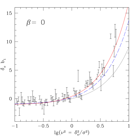
Figure 1: Large-scale linear bias factor associated with a barrier of constant height $\delta_{\rm c}$. Symbols with error bars show the bias factor determined via Monte-Carlo solution of equation (3), for walks with correlated steps because of Gaussian smoothing and $P_{\delta}(k)\propto k^{-1.2}$. I.e., $\delta_{\rm c}b_{1}$ was determined by considering walks conditioned to pass through $\delta\ll\delta_{\rm c}$ on scale $S\ll\delta_{\rm c}^{2}$, for a range of choices of $\delta$. Specifically, we show $[f(s|\delta,S)/f(s)-1]/(\delta/\delta_{\rm c})$ for $S=(0.15\delta_{\rm c})^{2}$ and $\delta/\delta_{\rm c}$ bin centers ranging from $[-1.8,-0.2]\sqrt{S}$, and from $[0.2,1.8]\sqrt{S}$, in steps of $0.4\sqrt{S}$, each of width $0.2\sqrt{S}$. (For clarity, at each $\nu$, symbols for different $\delta$ have been offset slightly.) Dotted curve shows $\delta_{\rm c}b_{u}=\nu^{2}-1$, which would be appropriate for walks with uncorrelated steps (equation 4). Solid curve shows the result of inserting equation (24) with $\Gamma_{\rm PH}=4.3$ in equation (19). Dashed curve shows $\delta_{\rm c}b_{1}$ determined from equation (24) of Ma et al. (2011) with their $\kappa=0.35$.

2.5 Comparison with Monte-Carlo solution

To test our analysis, Figure 1 compares the bias factor we measure by direct Monte-Carlo simulation of $b_{1}$ via equation (3). I.e., we construct the first crossing distribution of $B(s)=\delta_{\rm c}$ by walks conditioned to pass through some $\delta\ll\delta_{\rm c}$ on scale $S\ll\delta_{\rm c}^{2}$. Then we divide this by the (Monte-Carlo estimate of the) unconditional first crossing distribution, and subtract 1. Our Monte-Carlos assumed a power spectrum of the form $P_{\delta}(k)\propto k^{-1.2}$ and Gaussian smoothing filters, for which $S_{\times}/S\to 2^{0.9}$ and $\Gamma_{\rm PH}=4.3$. The solid curve shows the result of inserting equation (24) with $\Gamma_{\rm PH}=4.3$ in equation (19). It provides an excellent description of our measurements. The dotted curve shows the bias relation for uncorrelated walks (i.e. a sharp-$k$ filter), equation (4), is noticably different, lying well below the measurements at high $\delta_{\rm c}/\sigma$.

The dashed curve shows the corresponding expression for the bias from Ma et al. (2011): the right hand side of their equation (24) minus 1, times $\delta_{\rm c}$. Their expression has one free parameter, $\kappa$; we set it to 0.35, the value they say is appropriate for Gaussian smoothing filters. Notice that, although it is not as good a description of our measurements as is our solid curve, it does a reasonable job, indicating that the technical machinery which went into generating this prediction has produced a reasonably accurate result. However, this same technical machinery has obscured the reason why their formula predicts a bias factor that is approximately twice as large as that given by equation (4) when $\delta_{\rm c}/\sigma\gg 1$. Ma et al. attribute this difference to what they call stochasticity in the barrier height – but this cannot be correct, because stochasticity is not present in our constant barrier Monte-Carlos.

To make this point more directly, note that on the large scales which are appropriate for the bias calculation, our analysis shows that the conditional distribution $f(s|\delta,S\to 0)$ should be very well approximated by the unconditional distribution $f(s)$ with a shift of origin by $(S_{\times}/S)\,\delta$. Upon noting that Ma et al.’s $\kappa$ is our $S_{\times}/S-1$, it is easy to show that their equation (A32) for $f(s|\delta,S\to 0)$, is indeed what our analysis suggests, except that they have used their own expression for $f(s)$, and the result has been expanded to lowest order in $\kappa$. However, this expansion in $\kappa$ has obscured the simple, intuitive relation between the conditional and unconditional distributions that our analysis exploits (e.g. Ma et al. themselves failed to notice it). This also explains why their expression for the bias factor does not provide as good a description of our Monte-Carlos as does ours: their expression assumes $\kappa\ll 1$ when it is not (this matters more than the fact that their expression for $f(s)$ is not as accurate as ours).

The results of the previous section suggest that the main difference between the solid and dotted curves (for Gaussian and sharp-$k$ filtered walks) is almost entirely due to the fact that the excursion set measurement yields a real-space bias factor which carries an additional factor of $S_{\times}/S$: for our Gaussian smoothed walks, this factor is $2^{0.9}$, whereas it is unity for the sharp-$k$ filter associated with equation (4). To show this explicitly, Figure 2 shows the result of dividing our measurement by $S_{\times}/S$ so as to compare it with the derivative of the unconstrained first crossing distribution, which we compute analytically using equation (24), and show as a solid curve. Notice that now the measurements (and our solid curve) are much closer to the dotted curve (which shows equation 4). The differences between the solid and dotted curves in this plot are entirely a consequence of the fact that the underlying first crossing distributions are different; they are a much fairer depiction of the effect of correlated steps on the large scale bias. The graphic differences between Figures 1 and 2 demonstrate explicitly that correctly accounting for the factor of $S_{\times}/S$ is essential; failure to do so leads to incorrect conclusions about the nature of the relationship between the derivative of the first crossing distribution and the large scale bias.

Figure 3 shows a similar analysis of the bias associated with a linearly decreasing barrier (we set $\alpha=1$ and $\beta=-1$). In this case, $b_{u}$ of equation (4) lies well below the Monte-Carlo solution, whereas $b_{1}$ of equation (24) lies above it, at least at small $\delta_{\rm c}/\sigma$. However, the $\Gamma_{\rm PH}\to\infty$ limit of equation (24), namely $\partial\ln f_{\rm c}(s)/\partial\delta_{\rm c}$ from equation (26), provides an excellent description. This is very reassuring because, as we remarked previously, $f_{\rm c}(s)$ itself (the $\Gamma_{\rm PH}\to\infty$ limit of the first crossing distribution) also provides a better description of the Monte-Carloed first crossing distribution. We note again that accounting for the factor of $S_{\times}/S$ was crucial.

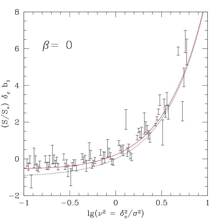
Figure 2: Same as previous Figure, except that now we have rescaled all quantities by a factor of $S/S_{\times}$. For the measurements and the solid curve, this factor is $1/2^{0.9}$; for the dotted curve it is $1$.

3 Discussion

We have presented an analysis of the large scale bias factor associated with the Excursion Set approach for smoothing filters which give rise to walks with correlated steps. This required careful consideration of the differences between real and Fourier space bias – something that has been all but ignored to date since, for a sharp-$k$ filter, these two are the same. For other filters, the real-space bias will generically be different.

In particular, our analysis shows that the first crossing distribution $f(s|\delta,S)$, of walks that are constrained to pass through $\delta$ on scale $S$ should, as $S\to 0)$, be very well approximated by the unconditional distribution $f(s)$ with a shift of origin by $(S_{\times}/S)\,\delta$ (equations 8 and 9). Thus, memory effects in the walks manifest in two conceptually different ways: the fact that $S_{\times}/S\neq 1$, and that the functional form of $f(s)$ itself is altered. We argued that the former is simply associated with smoothing effects associated with the precise way in which the bias factor was defined; the latter is the more fundamental difference. The usual procedure of differentiating the mass function with respect to the height of the walk on large scales provides a good description of the latter, which we identified with the Fourier-space bias factor; it underestimates the real-space bias estimated by the cross correlation between halos and the mass (smoothed on large scales), by a factor $S_{\times}/S$ that can be as large as 2 (equation (23); this factor is slightly smaller for $\Lambda$CDM-like power spectra), while slightly overestimating the bias from real-space correlation functions (equation (29)).

Comparison with measurements in Monte Carlo simulations of constrained random walks showed good quantitative agreement with our excursion set predictions of the real-space bias. In particular, the effect of the $S_{\times}/S$ term (the first of our two effects) can be large (compare the solid and dotted curves in Figure 1). The fact that the first crossing distribution $f$ (equation (15)) is not the same as the one for uncorrelated steps $f_{u}$ (equation (2)) also matters, though it is subdominant (solid and dotted curves in Figure 2 are different, but this difference is smaller than in Figure 1). However, this second effect is the only one which matters for the Fourier space bias. The agreement between the solid curves and the measurements in Figures 1 and 2 suggest that any additional effects missed by our analysis must be small.

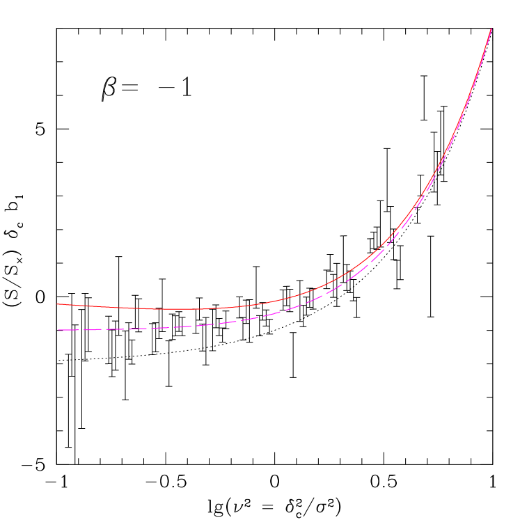
Figure 3: Same as Figure 2 except now the barrier is $B(s)=\delta_{\rm c}(1+\beta s/\delta_{\rm c}^{2})$. Symbols with error bars show the bias factor determined via Monte-Carlo solution of equation (3); dotted curve shows the prediction for walks with uncorrelated steps (from equation 4); solid curve shows equation (24), and dashed curve shows $\partial\ln f_{\rm c}(s)/\partial\ln\delta_{\rm c}$ (from equation (26)), which is the $\Gamma_{\rm PH}\to\infty$ limit of equation (24).

Our results highlight the fact that, when bias is simple in Fourier space, then, once one goes beyond sharp-$k$ smoothing, almost all measures of the large-scale bias factor will differ from one another, but these differences can be understood simply as a result of applying different smoothing filters to the same underlying Fourier space bias. Differences between real and Fourier space measures of the large scale bias factor are now being seen in simulations (e.g. Manera et al. 2010), so future comparison of these bias factors with simulations should be careful to specify which measure of the bias is actually being studied.

We noted that our excursion set calculation of the difference between real and Fourier space bias is consistent with the differences between real and Fourier space bias for peaks reported by Desjacques et al. (2010). The peaks calculation is remarkable because there, the bias factors are $k$-dependent. We believe that one of the virtues of our excursion set analysis is that it shows clearly how the excursion set approach too can lead to $k$-dependent bias. Namely, if halos of mass $m$ formed from peaks in the initial density field, then one would replace equation (9) with the expression which describes the density run around peaks rather than random positions of height $\delta_{\rm c}/\sigma(m)$. This would yield real-space bias factors which, following Desjacques et al. (2010), could then be interpreted in terms of $k$-dependent bias in Fourier space, in effect providing the first calculation of $k$-dependent bias from excursion set theory.

Appendix A Halo-mass cross correlation with Fourier-space biasing

When the halo field in Fourier-space is linearly biased as in equation (20) with $\delta_{\rm pk}\to\delta_{h}$ and $R_{\rm pk}\to R_{h}$, and with a constant bias $b$, then the bias determined from the ratio of the halo-mass cross correlation $\xi_{\rm hm}$ and the mass autocorrelation function $\xi_{\rm mm}$, will in general be smaller than $b$. To see this, consider a toy model for the CDM power spectrum given by $P_{\delta}(k)\propto k\,{\rm e}^{-k^{2}R_{\rm C}^{2}/2}$. Further assuming the halo field in equation (20) to be Gaussian filtered with $W(kR_{h})={\rm e}^{-k^{2}R_{h}^{2}/2}$, we have

$$\xi_{\rm mm}(r;R_{\rm C}) \equiv\langle\,\delta_{m}(0)\delta_{m}({\bf r})\,\rangle$$

$$=\int\frac{{\rm d}k}{k}\,\frac{k^{3}P_{\delta}(k)}{2\pi^{2}}\,j_{0}(kr)$$

$$=\xi(r/R_{\rm C})\,,$$ (27)

$$\xi_{hm}(r;R_{\rm C},R_{h}) \equiv\langle\,\delta_{h}(0)\delta_{m}({\bf r})\,\rangle$$

$$=b\int\frac{{\rm d}k}{k}\,\frac{k^{3}P_{\delta}(k)}{2\pi^{2}}\,{\rm e}^{-k^{2}R_{h}^{2}/2}j_{0}(kr)$$

$$=b\left(1+\frac{R_{h}^{2}}{R_{\rm C}^{2}}\right)^{-2}\xi\left(r/\sqrt{R_{h}^{2}+R_{\rm C}^{2}}\right)\,,$$ (28)

with the same function $\xi(x)$ appearing in both expressions, but with different arguments. For $R_{h}\ll R_{\rm C}$ we can then write

$$\frac{\xi_{hm}}{\xi_{mm}}\simeq b\left[1-\left(2+\frac{1}{2}\frac{d\ln\xi}{d\ln x}\right)\frac{R_{h}^{2}}{R_{\rm C}^{2}}+\ldots\right]\,,$$ (29)

where $x=r/R_{\rm C}$. For separations $r$ such that $\xi(x)\propto x^{-(n+3)}$, this bias from correlation functions therefore picks up a relative decrement of $|\Delta b|/b\simeq(|n-1|/2)(R_{h}/R_{\rm C})^{2}$, whose magnitude depends on halo mass, becoming smaller for halos of smaller mass. This is qualitatively in agreement with the results of $N$-body simulations discussed by Manera et al. (2010).

References

- [1] Bond J. R., Cole S., Efstathiou G., Kaiser N., 1991, ApJ, 379, 440
- [2] Cole S., Kaiser N., 1989, MNRAS, 237, 1127
- [3] Desjacques V., Crocce M., Scoccimarro R., Sheth R. K., 2010, PRD, 82, 103529
- [4] Epstein R. I., 1983, MNRAS, 205, 207
- [5] Lacey C., Cole S., 1993, MNRAS, 262, 627
- [6] Lam T. Y., Sheth R. K., 2009, MNRAS, 398, 2143
- [7] Ma, C.-P., Maggiore M., Riotto A., Zhang J., 2011, MNRAS, 411, 2644
- [8] Maggiore M., Riotto A., 2010, ApJ, 711, 907
- [9] Manera M., Sheth R. K., Scoccimarro R., 2010, MNRAS, 402, 589
- [10] Mo H. J., White S. D. M., 1996, MNRAS, 282, 347
- [11] Paranjape A., Lam T. Y., Sheth R. K., 2011, arXiv:1105.1990, MNRAS, in press
- [12] Peacock J. A., Heavens A. F., 1990, MNRAS, 243, 133
- [13] Press W. H., Schechter P., 1974, ApJ, 187, 425
- [14] Sheth R. K., 1998, MNRAS, 300, 1057
- [15] Sheth R. K., Mo H. J., Tormen G., 2001, MNRAS, 323, 1
- [16] Sheth R. K., Tormen G., 1999, MNRAS, 308, 119