Theory of Raman Scattering in One-Dimensional Quantum Spin-$\frac{\bm{1}}{\bm{2}}$ Antiferromagnets

Abstract

We study theoretically the Raman scattering spectra in the one-dimensional (1D) quantum spin-$\frac{1}{2}$ antiferromagnets. The analysis reveals that their low-energy dynamics is exquisitely sensitive to various perturbations to the Heisenberg chain with nearest-neighbor exchange interactions, such as magnetic anisotropy, longer-range exchange interactions, and bond dimerization. These weak interactions are mainly responsible for the Raman scattering and give rise to different types of spectra as functions of frequency, temperature, and external field. In contrast to the Raman spectra in higher dimensions in which the two-magnon process is dominant, those in 1D antiferromagnets provide much richer information on these perturbations.

Introduction: Quantum antiferromagnets have long attracted much attention as a laboratory to study quantum many-body effects. Experimentally, several techniques are available to investigate them; measurements of magnetic susceptibility, specific heat, and spectra of neutron scattering, NMR, and ESR. Recently, the optical spectra Devereaux ; Lemmens ; Katsura ; Wang have also turned out to be a powerful tool to study quantum spin dynamics. An example is electromagnon spectroscopy of multiferroics, where the one-magnon process is activated by an electric field in infrared absorption due to the magnetostriction mechanism Wang . Raman scattering Devereaux ; Lemmens ; Fleury ; Moriya , on the other hand, is usually considered to detect two-magnon excitations in antiferromagnetic (AF) ordered phases, which has been utilized to estimate the strength of the exchange interaction.

In one-dimensional (1D) systems where quantum fluctuations are much enhanced, such a simple magnon picture fails miserably. A canonical model for 1D quantum antiferromagnets is the spin-$\frac{1}{2}$ Heisenberg Hamiltonian,

$${\cal H}_{0} = J\sum_{j}{\bm{S}}_{j}\cdot{\bm{S}}_{j+1},$$ (1)

where $J$ ($>0$) is the exchange interaction between neighboring spins. The low-energy physics of this system is described by a Tomonaga-Luttinger (TL) liquid with gapless spinon excitations Giamarchi instead of magnons. In real systems, however, additional small perturbations ${\cal V}$ always exist, e.g., spin-orbit interaction, magnetic anisotropy, disorder, longer-range exchange interactions, and also spin-lattice coupling leading to the bond dimerization (spin-Peierls instability). Despite the smallness of these interactions, they are crucial for the quantum dynamics of the system, and are the subject of intensive studies.

Unfortunately, experimental signatures of these small perturbations ${\cal V}$ are often difficult to study because conventional experiments probe quantities that are dominated by the Heisenberg term (1) of the Hamiltonian. Therefore, it is highly desirable to have experimental probes that reveal the physical processes associated with the small perturbations ${\cal V}$ in 1D antiferromagnetic systems. In this Letter, we show that Raman scattering from 1D spin-$\frac{1}{2}$ antiferromagnets provides such an experimental probe.

It has been considered so far that the Raman scattering in 1D magnets is not so useful compared to other conventional methods although some of the experimental and theoretical works exist Lemmens ; Muthukumar ; Lemmens2 ; Loosdrecht ; Ruckamp ; Schmidt ; Schmidt2 ; Orignac . This is because the Hamiltonian ${\cal H}_{0}$ and the corresponding Raman operator ${\cal R}_{0}\propto{\cal H}_{0}$ [see Eq. (3)] commute with each other, and hence no Raman scattering occurs without additional interactions. Furthermore, these perturbations ${\cal V}$, which determine the Raman scattering spectra (RSS), remain rather uncertain in most cases. However, this does not necessarily mean that the RSS is useless in these systems. In fact, once theoretical predictions on the RSS for each interaction ${\cal V}$ are available, RSS can provide useful information on ${\cal V}$ as we will see later.

The results of our analysis based on field-theory and nonperturbative methods are summarized in Tables 1 and Fig. 2 for gapless cases, and Table 2 and Fig. 3 for gapped cases, respectively. Comparing these predictions with the observed temperature, frequency, and magnetic-field dependence of the RSS, one can obtain detailed information on ${\cal V}$. The results will be explained below.

Definition of RSS: Let us start from the definition of the RSS and the Raman operator. The RSS is proportional to the dynamical structure factor of the Raman operator ${\cal R}$, namely,

$$I(\omega) = \frac{1}{2\pi}\int^{\infty}_{-\infty}dt\,\,e^{i\omega t}\langle{\cal R}(t){\cal R}(0)\rangle,$$ (2)

where $\omega=\omega_{i}-\omega_{s}$ and $\omega_{i(s)}$ is the energy of incident (scattered) photon. In Mott-insulating systems, the Raman operator Devereaux ; Lemmens ; Fleury ; Moriya usually has the form

$${\cal R} = \sum_{{\bm{r}}_{1},{\bm{r}}_{2}}({\bm{e}}_{i}\cdot{\bm{r}}_{12})({\bm{e}}_{s}\cdot{\bm{r}}_{12})A({\bm{r}}_{12}){\bm{S}}_{{\bm{r}}_{1}}\cdot{\bm{S}}_{{\bm{r}}_{2}},$$ (3)

where ${\bm{e}}_{i(s)}$ is the polarization direction of the incident (scattered) photon and ${\bm{r}}_{12}={\bm{r}}_{1}-{\bm{r}}_{2}$. Therefore, the RSS strongly depends on the direction of applied and observed electromagnetic waves and the crystal structure of magnets. The factor $A({\bm{r}}_{12})$ is difficult to accurately determine, but the ratio between the factors on different bonds is known to be of the same order as that between the exchange couplings on those bonds. From Eqs. (2) and (3), one can easily find that the intensity $I(\omega)$ is unchanged when ${\cal R}$ is replaced with the modified Raman operator

$${\cal R}^{\prime} = {\cal R}-C{\cal H},$$ (4)

where $C$ is arbitrary real constant and ${\cal H}$ is the Hamiltonian of the target magnet. We can therefore adopt ${\cal R}^{\prime}$ to make the calculation of $I(\omega)$ easier.

Analysis: The low-energy physics of the Heisenberg chain (1) with/without an easy-plane anisotropy ${\cal V}_{1}=-J\Delta\sum_{j}S_{j}^{z}S_{j+1}^{z}$ and a Zeeman term is well described by the TL-liquid theory Giamarchi . The low-energy effective Hamiltonian is identical to the free boson theory

$${\cal H}_{0}^{\rm eff} = \int dx\frac{v}{2}\left[K^{-1}(\partial_{x}\phi)^{2}+K(\partial_{x}\theta)^{2}\right],$$ (5)

where $x=ja_{0}$ ($a_{0}$ is lattice spacing), $v$ is the spinon velocity, $K$ is the TL-liquid parameter, and $(\phi,\theta)$ is the canonical pair of bosonic fields. The parameter $K=1$ at the SU(2) symmetric point, while an anisotropy ${\cal V}_{1}$ or an external field $H$ usually increases the value of $K$, i.e., $K>1$. Note that ${\cal V}_{1}$ is the perturbation in the sense that it violates the commuting property of the Hamiltonian ${\cal H}_{0}+{\cal V}_{1}$ and the Raman operator ${\cal R}$. Spin and dimer operators can also be bosonized as $S^{\alpha}_{j}\approx{\cal J}^{\alpha}(x)+(-1)^{j}{\cal N}^{\alpha}(x)$ and $(-1)^{j}{\bm{S}}_{j}\cdot{\bm{S}}_{j+1}\approx d\sin(\sqrt{2\pi}\phi)+\cdots$, where ${\cal N}^{+}=b_{0}e^{i\sqrt{2\pi}\theta}+\cdots$, ${\cal J}^{+}=b_{1}e^{i\sqrt{2\pi}\theta}\cos(\sqrt{2\pi}\phi)+\cdots$, ${\cal N}^{z}=a_{1}\cos(\sqrt{2\pi}\phi)+\cdots$, and ${\cal J}^{z}=a_{0}\partial_{x}\phi/\sqrt{2\pi}$. The anisotropy and field dependence of parameters $a_{1}$, $b_{0,1}$, $d$, $K$ and $v$ is accurately evaluated Lukyanov ; H-F ; T-S . The bosonization approach therefore enables us to estimate the effects of several perturbations on the RSS $I(\omega)$ with reasonable accuracy in the low-energy region, i.e., $T,|\omega|\ll J$.

Gapless Cases: Let us study four realistic perturbations ${\cal V}$ that do not violate the TL-liquid phase; XXZ anisotropy ${\cal V}_{1}$, longer-range exchange couplings ${\cal V}_{2}=\sum_{n\geq 2}\sum_{j}J_{n}{\bm{S}}_{j}\cdot{\bm{S}}_{j+n}$ ($|J_{n}|\ll J$), a bond tilting in Fig. 1, and a random bond alternation ${\cal V}_{4}=\sum_{j}J(-1)^{j}u_{j}{\bm{S}}_{j}\cdot{\bm{S}}_{j+1}$ with $u_{j}$ being the randomly distributed lattice distortion ($|u_{j}|\ll 1$). The results are summarized in Table 1 and Fig. 2.

Table 1: Properties of RSS $I(\omega)$ in gapless cases of 1D Heisenberg magnet ${\cal H}_{0}$ with perturbation ${\cal V}$. Constants $c_{1-12}$ depends on the TL-liquid parameter $K$, the spinon velocity $v$, the magnetization $M=\langle S_{j}^{z}\rangle$, the lattice spacing $a_{0}$, etc. The value of $K$ is unity at the SU(2)-symmetric case, while an easy-plane XXZ anisotropy or a magnetic field $H$ increases it, i.e., $K>1$.

perturbation ${\cal V}$	bosonized form of ${\cal V}$	scaling dimension	RSS $I(\omega)$	main effect of field $H$
XXZ anisotropy ${\cal V}_{1}=-J\Delta\sum_{j}S_{j}^{z}S_{j+1}^{z}$	$J\Delta({\cal N}^{z}{\cal N}^{z}-{\cal J}^{z}{\cal J}^{z})$	$2K$ (${\cal N}^{z}$ term) $2$ (${\cal J}^{z}$ and ${\cal N}^{z}$ terms)	$c_{1}\omega^{4K-2}+c_{2}\omega^{2}$ ($\beta\omega\gg 1$) $c_{3}T^{4K-2}+c_{4}T^{2}$ ($\beta\omega\ll 1$)	$c_{1,3}$ terms disappear in $\omega\lesssim\omega_{1}=4\pi Mv/a_{0}$
longer-range coupling ${\cal V}_{2}=\sum_{j}J_{n}{\bm{S}}_{j}\cdot{\bm{S}}_{j+n}(n\geq 2)$	$c_{xy}({\cal J}_{R}^{+}{\cal J}_{L}^{-}+{\rm h.c.})/2$ $+c_{z}{\cal J}_{R}^{z}{\cal J}_{L}^{z}$	$2K$ ($c_{xy}$ term) $2$ ($c_{z}$ term)	$c_{5}\omega^{4K-2}+c_{6}\omega^{2}$ ($\beta\omega\gg 1$) $c_{7}T^{4K-2}+c_{8}T^{2}$ ($\beta\omega\ll 1$)	$c_{5,7}$ terms disappear in $\omega\lesssim\omega_{1}$
tilting bond in Fig. 1	$\sin(2\theta_{0})\sin(\theta_{i}+\theta_{s})$ $\times d\sin(\sqrt{2\pi}\phi)$	$K/2$	$c_{9}\omega^{K-2}$ ($\beta\omega\gg 1$) $c_{10}T^{K-2}$ ($\beta\omega\ll 1$)	$c_{9,10}$ terms disappear in $\omega\lesssim\omega_{2}=2\pi Mv/a_{0}$
random dimerization ${\cal V}_{4}=\sum_{j}J(-1)^{j}u_{j}{\bm{S}}_{j}\cdot{\bm{S}}_{j+1}$	$Ju_{j}d\sin(\sqrt{2\pi}\phi)$	$K/2$	$c_{11}\omega^{K-1}$ ($\beta\omega\gg 1$) $c_{12}T^{K-1}$ ($\beta\omega\ll 1$)	value of $K$ increases

Generally ${\cal V}_{1,2}$ are always present in real compounds. The main part of the bosonized ${\cal V}_{2}$ is

$$\int\frac{dx}{a_{0}}\,\,\frac{c_{xy}}{2}({\cal J}_{R}^{+}{\cal J}_{L}^{-}+{\rm h.c.})+c_{z}{\cal J}_{R}^{z}{\cal J}_{L}^{z}$$ (6)

where ${\cal J}_{R(L)}^{\alpha}$ is the right (left) moving part of ${\cal J}^{\alpha}$, and constants $c_{xy}=c_{z}$ depend on $J$ and $J_{n}$. Similarly, we obtain ${\cal V}_{1}\approx-J\Delta\int\frac{dx}{a_{0}}({\cal J}^{z}{\cal J}^{z}-{\cal N}^{z}{\cal N}^{z})$. From Eq. (4), we can make ${\cal R}^{\prime}$ proportional to ${\cal V}_{1,2}$ if ${\bm{e}}_{i,s}$ are set parallel to ${\bm{r}}_{j}-{\bm{r}}_{j+1}$. Applying the standard technique based on the bosonization and conformal field theory Giamarchi , we can calculate the Raman intensity of the Heisenberg chain ${\cal H}_{0}$ with ${\cal V}_{1}$ or ${\cal V}_{2}$ for arbitrary frequency $\omega$ and temperature $T=1/\beta$. The result for the case of ${\cal V}_{2}$ is

$$I(\omega) \propto 2c_{xy}^{2}F(\omega,\beta,K)+c_{z}^{2}F(\omega,\beta,1+\epsilon)|_{\epsilon\to 0}$$ (7)

where $F(x,y,z)=\frac{a_{0}}{2\pi v}(1-e^{-xy})^{-1}\sin(2\pi z){\rm Im}[B(-i\frac{xy}{4\pi}+z,1-2z)^{2}](\frac{2\pi a_{0}}{yv})^{4z-2}$ and $B(x,y)$ is the Beta function. We also have $I(\omega)\propto\frac{1}{2}\pi^{2}a_{1}^{4}F(\omega,\beta,K)+K^{2}(\frac{1}{2\pi}+\frac{\pi}{2}a_{1}^{2})^{2}F(\omega,\beta,1+\epsilon)$ for the case of ${\cal V}_{1}$. The intensities of these two cases are presented in Fig. 2 (a) and (b), and they show that $I(\omega)$ is a monotonically increasing function of $\omega$, and it remains finite in the limit $\omega/J\to 0$ at finite temperatures. These properties are at least qualitatively consistent with the experimental result of the paramagnetic phase of $\rm CuGeO_{3}$ Muthukumar ; Lemmens2 , in which $J\sim 150$K and $J_{2}\sim 30$K. We note that ${\cal V}_{1}$ and ${\cal V}_{2}$ give the similar behavior in the RSS, but they can be distinguished by other physical quantities such as susceptibilities. When we apply a magnetic field $H$ and a magnetization $M=\langle S_{j}^{z}\rangle$ appears, $B(-i\frac{\beta\omega}{4\pi}+K,1-2K)^{2}$ in the first term $F(\omega,\beta,K)$ of $I(\omega)$ is changed into $B(-i\frac{\beta(\omega+4\pi Mv/a_{0})}{4\pi}+K,1-2K)B(-i\frac{\beta(\omega-4\pi Mv/a_{0})}{4\pi}+K,1-2K)$ for both cases of ${\cal V}_{1,2}$. As a result, the RSS weight of this term becomes nearly zero in the low-frequency region $\omega\lesssim\omega_{1}=4\pi Mv/a_{0}$ at low temperatures $T\ll J$. For instance, in the case of ${\cal V}_{2}$, only the $c^{2}_{z}$ term survives in Eq. (7).

We next consider 1D magnets with a tilting bond as in Fig. 1. In fact, tilting structures with a small angle $\theta_{0}$ exist in several cuprate magnets such as Cu benzoate Dender , $\rm KCuGaF_{6}$ Umegaki , and $\rm[PM]Cu(NO_{3})_{2}(H_{2}O)_{2}$ (PM=pyrimidine) Feyerherm . In this system, the Hamiltonian is the same as Eq. (1) and hence a TL-liquid state survives. However, if we fix ${\bm{e}}_{i,s}$ as in Fig. 1, the Raman operator becomes different from that of the case without a tilting bond. Tuning the value of $C$ in Eq. (4), we obtain

$${\cal R}^{\prime} \propto \sin(2\theta_{0})\sin(\theta_{i}+\theta_{s})\sum_{j}(-1)^{j}{\bm{S}}_{j}\cdot{\bm{S}}_{j+1}.$$ (8)

This is nothing but a dimerization operator and does not commute with ${\cal H}_{0}$. Using this operator, we obtain $I(\omega)\propto\sin^{2}(2\theta_{0})\sin^{2}(\theta_{i}+\theta_{s})d^{2}F(\omega,\beta,K/2)$ that is depicted in Fig. 2 (c) note1 . The RSS rapidly increases around $\omega=T$ at low temperatures, and the form is quite different from the case of ${\cal V}_{1,2}$. Physically the origin of this spectrum is two-spinon states. We emphasize that the strength of $I(\omega)$ can be controlled by tuning angles $\theta_{i,s}$. Similarly to the case of ${\cal V}_{1,2}$, a magnetic field $H$ makes the weight of $I(\omega)$ absent in the region $\omega\lesssim\omega_{2}=2\pi Mv/a_{0}$.

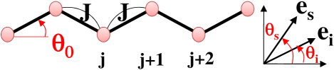
Figure 1: (color online) 1D antiferromagnet with tilting angle $\theta_{0}$ and polarization directions of incident and scattering photon ${\bm{e}}_{i,s}$ with angles $\theta_{i}$ and $\theta_{s}$.

A random dimerization is expected to be present in the higher-temperature paramagnetic phase of spin-Peierls compounds such as $\rm CuGeO_{3}$ Muthukumar and $\rm TiOCr$ Ruckamp . In this case, the Raman operator ${\cal R}^{\prime}$ is proportional to ${\cal V}_{4}/J\approx\int\frac{dx}{a_{0}}u_{j}d\sin(\sqrt{2\pi}\phi)$. Under the assumption that $u_{j}$ is a sufficiently small perturbation from ${\cal H}_{0}$ and $\langle u_{j}u_{k}\rangle_{R}={\bar{u}}^{2}\delta_{jk}$ ($\langle\cdots\rangle_{R}$ stands for the average over the randomness). the Raman intensity $\langle I(\omega)\rangle_{R}$ is reduced to a local correlator $\propto{\bar{u}}^{2}d^{2}\int\frac{dt}{2\pi}e^{i\omega t}\langle\sin(\sqrt{2\pi}\phi(t))\sin(\sqrt{2\pi}\phi(0))\rangle$. It is calculated as

$$\frac{{\bar{u}}^{2}d^{2}a_{0}}{4\pi v}\left(\frac{2\pi a_{0}}{\beta v}\right)^{K-1}e^{\frac{\beta\omega}{2}}B\left(\frac{K}{2}-i\frac{\beta\omega}{2\pi},\frac{K}{2}+i\frac{\beta\omega}{2\pi}\right),$$ (9)

which is shown in Fig. 2 (d). The $\omega$ dependence of $\langle I(\omega)\rangle_{R}$ is negligible in $\omega>T$. Such a spectrum with a small slope is observed in the paramagnetic phase of $\rm CuGeO_{3}$ (see the region $\omega\lesssim 50{\rm cm}^{-1}$ in Fig. 1 of Ref. Muthukumar, ), and therefore the spectrum might contain the contribution from ${\cal V}_{4}$. An applied field $H$ does not affect the form of $\langle I(\omega)\rangle_{R}$ much, but it slightly varies parameters $(K,v,a_{1},b_{0,1},d)$.

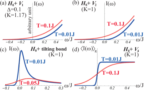
Figure 2: (color online) RSS $I(\omega)$ for 1D Heisenberg magnet (1) with additional perturbation ${\cal V}$s. Panels (a), (b), (c) and (d) correspond to the cases of ${\cal V}_{1}$, ${\cal V}_{2}$, the bond tilting in Fig. 1, and ${\cal V}_{4}$, respectively. All the continuous spectra come from multiple spinon states in the TL liquid phase.

Gapped Cases: Let us now discuss another kind of typical perturbations ${\cal V}$ that break the TL liquid in ${\cal H}_{0}$ and open a finite excitation gap: a static bond alternation (dimerization) term ${\cal V}_{5}=\sum_{j}J(-1)^{j}u{\bm{S}}_{j}\cdot{\bm{S}}_{j+1}$, and uniform and staggered Zeeman terms ${\cal V}_{6}=-\sum_{j}HS_{j}^{z}+(-1)^{j}hS_{j}^{x}$ induced by an applied field $H$. The results are summarized in Table 2 and Fig. 3.

Table 2: Properties of RSS $I(\omega)$ in gapped cases of 1D Heisenberg magnet ${\cal H}_{0}$ with perturbation ${\cal V}$ at $T=0$. In the case of ${\cal V}_{5}$, the soliton mass, and first and second breather masses are respectively evaluated as $E_{s}\approx 1.5u^{2/3}J$, $E_{1}=E_{s}$ and $E_{2}=\sqrt{3}E_{s}$, while $E_{s}\approx 2.1(h/J)^{2/3}J$ in the case of ${\cal V}_{6}$ with a small field $H\ll J$. Note that in the case of ${\cal V}_{5}$, $E_{2}$ becomes larger than $\sqrt{3}E_{s}$ Schmidt if the marginal operator, neglected in the SG model ${\cal H}_{5}$, is taken into account. On the other hand, a small next-nearest-neighbor AF coupling $J_{2}$ weakens the effect of the marginal term Schmidt .

perturbation ${\cal V}$	bosonized form of ${\cal V}$	Raman active mode (its main origin)	peak positions for each mode
static dimerization ${\cal V}_{5}=\sum_{j}J(-1)^{j}u{\bm{S}}_{j}\cdot{\bm{S}}_{j+1}$	$Jud\sin(\sqrt{2\pi}\phi)$	second breather ($\sin(\sqrt{2\pi}\phi)$ term) ${\cal S}$-$\bar{\cal S}$ continuum ($\sin(\sqrt{2\pi}\phi)$ term)	$\omega=E_{2}$ (stable against $H$) $\omega\geq 2E_{s}$
uniform and staggered Zeeman terms ${\cal V}_{6}=-\sum_{j}HS_{j}^{z}+(-1)^{j}hS_{j}^{x}$	$-Ha_{0}\partial_{x}\phi/\sqrt{2\pi}$ $-hb_{0}\cos(\sqrt{2\pi}\theta)$	soliton, antisoliton (tilting bond) odd-th breathers ($\partial_{x}\phi$ term) even-th breathers ($\cos(\sqrt{2\pi}\theta)$ term)	$\omega=(E_{s}^{2}+(2\pi Mv/a_{0})^{2})^{1/2}$ $\omega=E_{2n+1}$ $\omega=E_{2n}$

In the case of ${\cal V}_{5}$, the effective Hamiltonian becomes an exactly solvable sine-Gordon (SG) model,

$${\cal H}_{5} = {\cal H}_{0}^{\rm eff}+\int\frac{dx}{a_{0}}ud\sin(\sqrt{2\pi}\phi).$$ (10)

There are three kinds of massive excitations: soliton (${\cal S}$), antisoliton ($\bar{\cal S}$), and some breathers (${\cal B}_{n}$) that are the soliton-antisoliton bound states. The mass of the soliton $E_{s}$ is equal to that of antisoliton, and it is given by T-S

$$\frac{E_{s}}{J}=\frac{v}{Ja_{0}}\frac{2}{\sqrt{\pi}}\frac{\Gamma(\frac{K}{8-2K})}{\Gamma(\frac{2}{4-K})}\left[\frac{Ja_{0}}{v}\frac{\pi d}{2}\frac{\Gamma(\frac{4-K}{4})}{\Gamma(K/4)}\right]^{\frac{2}{4-K}},$$ (11)

where $\Gamma(x)$ is the Gamma function. The $n$-th breather’s mass $E_{n}$ is related to $E_{s}$ via $E_{n}=2E_{s}\sin[n\pi/(8/K-2)]$ with $n=1,\cdots,[4/K-1]$. The SU(2)-symmetric dimerized chain with $K=1$ has only two breathers ${\cal B}_{1,2}$. Three particles ${\cal S}$, $\bar{\cal S}$ and ${\cal B}_{1}$ corresponds to massive spin-1 triplet excitations with $S^{z}=+1$, $-1$, and $0$, respectively, while ${\cal B}_{2}$ is regarded as a singlet excitation with $S=0$. The soliton mass is evaluated as $E_{s}\approx 3.5(du)^{2/3}J$ with $d\approx 0.3$ T-S at the SU(2) point. From Eq. (3), the RSS is proportional to the dynamical structure factor of $\sin(\sqrt{2\pi}\phi)$. To accurately evaluate such dynamical correlators of the SG model at the low-energy region, we utilize the form-factor approach E-K ; K-E which is reliable when $T/J\ll 1$. From this approach, the lowest-frequency contribution of $I(\omega)$ is shown to be a $\delta$-functional peak of the singlet breather ${\cal B}_{2}$ at $\omega=E_{2}$, and the second lowest one is given by the continuum spectrum of soliton-antisoliton scattering states with $\omega\geq 2E_{s}$. The weight of each contribution can also be exactly calculated by the form-factor method. In particular, the weight of the singlet breather is proportional to $(E_{s}a_{0}/v)^{K}$, and is much larger than that of the continuum. The ${\cal B}_{2}$ peak and its weight in $I(\omega)$ are shown in Fig. 3 (a). The distortion ($u$) dependence of this peak can be compared to Raman scattering experiments for spin-Peierls magnets, $\rm CuGeO_{3}$ Muthukumar ; Loosdrecht , $\rm TiOCr$ Ruckamp , etc. The ${\cal B}_{2}$ peak of $I(\omega)$ is stable against an applied field $H$ if $H$ is smaller than the critical field $H_{c}=E_{s}$.

A staggered magnetic field $h$ emerges as we apply a uniform field $H$ to magnets with a staggered gyromagnetic tensor O-A . Typical examples are Cu benzoate Dender , $\rm KCuGaF_{6}$ Umegaki , and $\rm[PM]Cu(NO_{3})_{2}(H_{2}O)_{2}$ Feyerherm , in which a tilting structure is also present (as we discussed). In these compounds, $h\approx c_{s}H$ ($|c_{s}|\ll 1$) is realized. The bosonized form of ${\cal V}_{6}$ is given by

$$-Ha_{0}\partial_{x}\phi/\sqrt{2\pi}-hb_{0}\cos(\sqrt{2\pi}\theta).$$ (12)

The term $\partial_{x}\phi$, inducing a finite $M$, can be absorbed into the free boson part ${\cal H}_{0}^{\rm eff}$, and then the effective Hamiltonian is also a SG model O-A . Therefore, we can again apply the form-factor method to calculate $I(\omega)$. The soliton mass is given by Eq. (11) with replacing $(K,d)$ by $(1/K,hb_{0})$, and the breather masses are given by $E_{n}=2E_{s}\sin[n\pi/(8K-2)]$ with $n=1,\cdots,[4K-1]$. Since the value of $K$ increases with increasing $H$, the number of breathers $[4K-1]$ is also increased with $H$ in the present case. From the form-factor method K-E , $\partial_{x}\phi$, $\cos(\sqrt{2\pi}\theta)$, and the tilting-bond term $\sin(\sqrt{2\pi}\phi)$ in the Raman operator are respectively shown to provide $\delta$-functional peaks of odd-th breathers at $\omega=E_{\rm odd}$, even-th breathers at $\omega=E_{\rm even}$, and soliton (antisoliton) with wavenumber $k=2\pi M/a_{0}$ at $\omega=(E_{s}^{2}+k^{2}v^{2})^{1/2}$ in the spectrum $I(\omega)$. Namely, in contrast to the case of ${\cal V}_{5}$, all of the elementary particles of the SG model can be observed. The $H$ dependence of several peak positions are plotted in Fig. 3 (b). Remarkably, level crossings between soliton and breather peaks occur Umegaki . In addition to these peaks, there exist continuum spectra with a smaller weight, although it is difficult to accurately evaluate them.

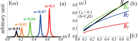
Figure 3: (color online) (a) $u$ dependence of the singlet-breather (${\cal B}_{2}$) peak in $I(\omega)$ of the dimerized magnet ${\cal H}_{0}+{\cal V}_{5}$ at $T=0$, where $\delta$ functions are broadened. The peak position $\omega=E_{2}$ and its weight are both proportional to $u^{2/3}$. This peak is stable against an applied field $H$. The weight of the continuum spectrum with $\omega\geq 2E_{s}$ is much smaller than that of the ${\cal B}_{2}$ peak, and the former is omitted here. (b) $H$ dependence of peak positions of each particle in $I(\omega)$ of the magnet ${\cal H}_{0}+{\cal V}_{6}$ at $T=0$. Some level crossings between the soliton ${\cal S}$ and breather ${\cal B}_{n}$ peaks occur with increasing $H$. The continuum spectra are omitted.

In conclusion, we have shown that various weak perturbations ${\cal V}$ to the spin-$\frac{1}{2}$ AF Heisenberg Hamiltonian, which are expected to determine the quantum dynamics in different real 1D antiferromagnets, will have distinctive spectral responses in Raman scattering studies of 1D antiferromagnets. The results summarized in Tables 1 and 2 provide a means of obtaining useful information about different perturbations by comparing our results with future experimental results.

This work is supported by Grant-in-Aids for Scientific Research (No. 21244053, No. 21740295, No. 22014016, and No. 23740298) from the Ministry of Education, Culture, Sports, Science and Technology of Japan, and also by Funding Program for World-Leading Innovative R&D on Science and Technology (FIRST Program).

References

• (1) See, for a review, T.P. Devereaux, and R. Hackl, Rev. Mod. Phys. 79, 175 (2007).
• (2) See, for a review, P. Lemmens, G. Gรผntherodt, and G. Gros, Phys. Rep. 375, 1 (2003).
• (3) H. Katsura, M. Sato, T. Furuta, and N. Nagaosa, Phys. Rev. Lett. 103, 177402 (2009).
• (4) See, for a review, K.F. Wang, J.-M. Liu, and Z.F. Ren, Advances in Physics 58, 321 (2009).
• (5) P.A. Fleury and R. Loudon, Phys. Rev. 166, 514 (1968).
• (6) T. Moriya, J. Phys. Soc. Jpn. 23, 490 (1967); J. App. Phys. 39, 1042 (1968).
• (7) T. Giamarchi, Quantum Physics in One Dimension (Oxford Univ. Press, New York, 2004).
• (8) V.N. Muthukumar, C. Gros, W. Wenzel, R. Valentรญ, P. Lemmens, B. Eisener, G. Gunฬˆtherodt, M. Weiden, C. Geibel, and F. Steglich, Phys. Rev. B 54, R9635 (1996).
• (9) P. Lemmens, M. Fischer, and G. Gรผntherodt, C. Gros, P. G. J. van Dongen, M. Weiden, W. Richter, C. Geibel, and F. Steglich, Phys. Rev. B 55, 15076 (1997).
• (10) P. H. M. van Loosdrecht, J. Zeman, G. Martinez, G. Dhalenne, and A. Revcolevschi, Phys. Rev. Lett. 78, 487 (1997).
• (11) R. Rรผckamp, J. Baier, M. Kriener, M. W. Haverkort, T. Lorenz, G. S. Uhrig, L. Jongen, A. Mรถller, G. Meyer, and M. Grรผninger, Phys. Rev. Lett. 95, 097203 (2005).
• (12) K.P. Schmidt, C. Knetter, and G.S. Uhrig, Phys. Rev. B 69, 104417 (2004). 113 (2000).
• (13) K.P. Schmidt, C. Knetter, and G.S. Uhrig, Europhys. Lett. 56, 877 (2001).
• (14) E. Orignac, R. Citro, S. Capponi, and D. Poilblanc, Phys. Rev. B 76, 144422 (2007).
• (15) S. Lukyanov and A.B. Zamolodchikov, Nucl. Phys. B 493, 571 (1997).
• (16) T. Hikihara and A. Furusaki, Phys. Rev. B 58, R583 (1998); Phys. Rev. B 69, 064427 (2004).
• (17) S. Takayoshi and M. Sato, Phys. Rev. B 82, 214420 (2010).
• (18) D.C. Dender, P.R. Hammar, D.H. Reich, C. Broholm, and G. Aeppli, Phys. Rev. Lett. 79, 1750 (1997).
• (19) I. Umegaki, H. Tanaka, T. Ono, H. Uekusa, and H. Nojiri, Phys. Rev. B 79, 184401 (2009).
• (20) R. Feyerherm, S. Abens, D. Gรผnther, T. Ishida, M. MeiรŸner, M. Meschke, T. Nogami, and M. Steiner, J. Phys.: Condens. Matter 12, 8495 (2000).
• (21) We have checked that the peak amplitude of the RSS per one spin for the 1D Heisenberg chain ${\cal H}_{0}$ with a small tilting angle (e.g., $\theta_{0}=\pi/18$) is comparable with that for the Nรฉel state of the 2D Heisenberg model with the same value of the exchange coupling $J$ in the low-temperature region $T/J\ll 1$. The latter RSS for the Nรฉel state can be evaluated by the standard spin-wave theory, and is dominated by two-magnon processes. The two-magnon RSSs have been detected in several AF ordered materials [See, e.g., M. G. Cottam and D. J. Lockwood, Light scattering in Magnetic Solids (John Wiley $\&$ Sons 1986)]. These facts strongly suggest that continuous RSSs can also be observed in real quasi-1D quantum magnets.
• (22) F.H.L. Essler and R.M. Konik, cond-mat/0412421.
• (23) I. Kuzmenko and F.H.L. Essler, Phys. Rev. B 79, 024402 (2009).
• (24) M. Oshikawa and I. Affleck, Phys. Rev. Lett. 79, 2883 (1997).