More about Base Station Location Games

Abstract

This paper addresses the problem of locating base stations in a certain area which is highly populated by mobile stations; each mobile station is assumed to select the closest base station. Base stations are modeled by players who choose their best location for maximizing their uplink throughput. The approach of this paper is to make some simplifying assumptions in order to get interpretable analytical results and insights to the problem under study. Specifically, a relatively complete Nash equilibrium (NE) analysis is conducted (existence, uniqueness, determination, and efficiency). Then, assuming that the base station location can be adjusted dynamically, the best-response dynamics and reinforcement learning algorithm are applied, discussed, and illustrated through numerical results.

1 Introduction

Mobile terminals (MTs) are currently gaining increased autonomy of decision to allow a better use of the available wireless resources. For example, MTs may choose their wireless access technology or the base station (BS) or access point to which they want to connect. We could imagine that this may be done in the future independently of the network operator owner of the BS. A mobile operator deploying BSs for a wireless network will have to deal with these new characteristics. If his goal is to maximize the traffic gathered by his own BSs, he will have to take into account the presence of competitor network operators when deciding on the location of BSs. If every operator involved has the same reasoning, this problem of BSs placement may be cast in the framework of game theory and more precisely in the context of location games.

The history of location games starts with the work of Hotelling [8] in which the notion of spatial competition in a duopoly situation is introduced. More precisely, two firms compete for benefits over a finite segment crowded with customers. This results in the partition of the segment into a convex area of influence for each firm. Plastria [12] gives an overview of optimization approaches to place new facilities in an environment with pre-existing facilities. A large overview on location games is also presented in [7]. Location games are extended to the context of wireless networks with works such as [1] and [2]. The main difference arising in this new context is the interaction between MTs due to the mutual interference they generate. This point makes the association problem between MTs and BSs complex. As an association between a MT and a BS depends on SINR, the association relies on the respective locations of the MT and the BS, but also on the MTs already connected to the BS. Whereas [2] focuses on the downlink case, in [1] the location of BSs and the association choice of the MTs is treated as a Stackelberg game [15] in the uplink case. The context of our work is similar to the one in [1] but several interesting results are obtained in the present paper. The main contributions of this paper can be summarized as follows:

• As in [1] MTs are assumed to operate in the uplink and to be distributed along a one-dimensional region. However, each MT is assumed to select the closest BS (e.g., based on measure given by a GPS -global positioning system- receiver). This leads to a convenient form for the BSs utility functions (Sec. 2.1). As a consequence, the existence of a pure Nash equilibrium can be made rigorously (Sec. 3.1).

• Due to the symmetry of the problem, multiple Nash equilibria generally exist. However, if the locations can be ordered (which is easy for one-dimension regions), the Nash equilibrium can be determined and checked to be unique (Sec. 3.3).

• By making the reasonable assumption that the BS heights are much less than the typical distance between the BSs, the game can be further simplified and shown to be a form of Cournot oligopoly [4].

• In the two-player case, the efficiency of the Nash equilibrium is studied by evaluating the price of anarchy [9]. The influence of deploying its BS in the first place is studied by considering a Stackelberg formulation of the problem (Sec. 4.1).

• Assuming that the BS locations can be adjusted dynamically (which would be relevant in scenario like the one of small cells where only some of the small BS have to be active), the best response dynamics and reinforcement learning algorithm [3][14][11] are performed (Sec. 5).

• The made assumptions lead to several interpretations which could be further analyzed in the light of a more general framework (e.g., in two-dimensional regions).

The remainder of the paper is organized as follows. Section 2 introduces the physical model and the parameters of the $K$-player game. Section 3 describes the Nash equilibrium of the game in the one-dimensional case. In Section 4, the Nash equilibrium, the Stackelberg equilibrium, and the social optimum are compared. Section 5 presents a way to reach equilibrium using best-response dynamics and reinforcement learning. Finally, Section 6 concludes this work.

2 Model

Consider a plane to which a frame $\mathbb{R}$ is attached. A MT $X$ located in a position $x\in\mathbb{R}^{2}$ in this plane is linked with a BS $X_{1}$ of height $\varepsilon$ situated in $x_{1}\in\mathbb{R}^{2}$, see Figure 1. We define the Signal to Noise Ratio (SNR) and the Signal to Interference plus Noise Ration (SINR) of this MT

$$SNR_{X}=\frac{P_{X}.h_{X_{1}}(x)}{\sigma_{X_{1}}^{2}},$$ (1)

$$SINR_{X}=\frac{P_{X}.h_{X_{1}}(x)}{\sigma_{X_{1}}^{2}+I_{X_{1}}(x)},$$ (2)

where $P_{X}$ is the transmission power of the MT $X$, i.e. the level of power chosen by the MT to transmit its signal. $\sigma_{X_{1}}^{2}$ is the power of the channel noise, $I_{X_{1}}(x)$ is some interference term, $h_{X_{1}}(x)$ is the attenuation introduced by the uplink channel from $X$ to $X_{1}$. Here, it is assumed that

$$h_{X_{1}}(x)=\left(\left|x-x_{1}\right|^{2}+\varepsilon^{2}\right)^{-\frac{\alpha}{2}},$$ (3)

where $\left|x\right|$ is the $\ell_{2}$-norm of $x$ and $\alpha\geq 2$ is the path-loss exponent, $\alpha=2$ corresponding to the free-space path-loss case. A higher value of $\alpha$ suits to worse channel conditions.

With Single User Decoding (SUD) at the BS $X_{1}$, there is no hierarchy for decoding the incoming signals at the BS. Hence, the signal from MT $X$ is decoded by taking into account the full interference and the uplink capacity between $X$ and $X_{1}$ may be written as

$$C_{X}=\log\left(1+SINR_{X}\right),$$ (4)

Without loss of generality, when several MTs are considered, it is assumed that $P_{X}$ does not depend on the MT and is normalized, i.e., $P_{X}=1$. Moreover, the channel conditions, described by (3), are the same for every MT and the noise power is constant $\sigma_{X_{1}}=\sigma$. With these assumptions, (4) becomes

$$C_{X}=\log\left(1+\frac{\left(\left|x-x_{1}\right|^{2}+\varepsilon^{2}\right)^{-\frac{\alpha}{2}}}{{\sigma}^{2}+I_{X_{1}}(x)}\right).$$ (5)

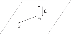
Figure 1: Base station located at $x_{1}$ and mobile station located at $x$

When several BSs are located on the plane, the MTs are assumed to be able to choose the BS they want to be linked with. In this paper, we consider that this association is made based on SNR. Given $\left(\ref{Eq:ChannelAttn}\right)$, choosing the BS with the highest SNR is equivalent to choosing the closest BS. Thus, it is assumed that a MT always chooses the closest BS to its location, leading to convex cells for BSs. For example, considering two BSs $X_{1}$ and $X_{2}$ at positions $x_{1}$ and $x_{2}$ and a MT $X$ at $x$, one has

$$C_{X}=\left\{\begin{array}[]{l}\log\left(1+\frac{(\left|x-x_{1}\right|^{2}+\varepsilon^{2})^{-\frac{\alpha}{2}}}{{\sigma}^{2}+I_{1}(x)}\right)\mbox{if }\left|x-x_{1}\right|^{2}\leqslant\left|x-x_{2}\right|^{2}\\ \log\left(1+\frac{(\left|x-x_{2}\right|^{2}+\varepsilon^{2})^{-\frac{\alpha}{2}}}{{\sigma}^{2}+I_{2}(x)}\right)\mbox{if }\left|x-x_{2}\right|^{2}\leqslant\left|x-x_{1}\right|^{2}.\end{array}\right.$$

2.1 Base station utility

The utility of a BS is taken as the sum of uplink capacities it offers to its connected users. We assume that the number of MT is large enough to be represented by a continuous distribution $\rho\left(x\right)$. This assumption allows to get the utility for the $k$-th BS as a continuous sum of the MTs uplink capacities

$$U_{k}(\underline{x})=\int_{S_{k}(\underline{x})}\rho(z)\log\left(1+\frac{(\left|z-x_{k}\right|^{2}+\varepsilon^{2})^{-\frac{\alpha}{2}}}{{\sigma}^{2}+I_{k}(\underline{x})}\right)\text{d}z,$$ (6)

where $S_{k}\left(\underline{x}\right)$ is the subset of the plane where MTs are linked with the $k$-th BS and $\underline{x}=~{}^{t}(x_{1},x_{2},\ldots,x_{K})$ is the vector of locations for the set of BSs. This paper will consider only uniform MT distribution with $\rho(x)=1$.

When considering interferences, a worst-case scenario is considered: there is no mechanism such as beamforming [10] to lower their effects. We consider that there is no interference between MTs connected with different BSs because of frequency reuse. Then only interference between MTs of a same BS has to be considered. This framework is quite similar to the one of [1], where two competing BSs are assumed to use different frequency bands. In our case, we consider $K$ BSs (with $K\geqslant 1$) and each of them uses its own frequency band.

Performing SUD at the $k$-th BS, one gets

$$I_{k}(\underline{x})=\int_{S_{k}(\underline{x})}\left(\left|z-x_{k}\right|^{2}+\varepsilon^{2}\right)^{-\frac{\alpha}{2}}\text{d}z.$$ (7)

Utility of $k$-th BS $\left(\ref{EqUtility1}\right)$ then becomes

$$U_{k}(\underline{x})=\int_{\mathcal{S}_{k}(\underline{x})}\log\left(1+\frac{(\left|z-x_{k}\right|^{2}+\varepsilon^{2})^{-\frac{\alpha}{2}}}{{\sigma}^{2}+\int_{\mathcal{S}_{k}(\underline{x})}(\left|z^{\prime}-x_{k}\right|^{2}+\varepsilon^{2})^{-\frac{\alpha}{2}}\text{d}z^{\prime}}\right)\text{d}z.$$ (8)

2.2 Utility approximation

When considering the low SINR regime, the useful power of each MT is small compared to the interference term in $\left(\ref{EqUtility2}\right)$. This is especially true for high MT density. With this assumption, $\left(\ref{EqUtility2}\right)$ may be approximated as

$$U_{k}(\underline{x}) \approx\frac{\int_{\mathcal{S}_{k}(\underline{x})}(\left|z-x_{k}\right|^{2}+\varepsilon^{2})^{-\frac{\alpha}{2}}{\text{d}z}}{{\sigma}^{2}+\int_{\mathcal{S}_{k}(\underline{x})}(\left|z^{\prime}-x_{k}\right|^{2}+\varepsilon^{2})^{-\frac{\alpha}{2}}{\text{d}z^{\prime}}}$$ (9)

$$=\frac{I_{k}(\underline{x})}{\sigma^{2}+I_{k}(\underline{x})}.$$

Note that this simplification makes the considered utility based on capacity equivalent to a utility based on SINR such as the ones in [1]. At low-SINR regime, it is equivalent to work with a capacity-based utility or a SINR-based utility.

Also note that one has $f\left(t\right)=t/\left(\sigma^{2}+t\right)$ strictly increasing over $\left[0,L\right]$, since its derivative is $f^{\prime}\left(t\right)=\sigma^{2}/\left(\sigma^{2}+t\right)^{2}$. Then maximizing the approximation of $U_{k}(\underline{x})$ or $I_{k}(\underline{x})$ is equivalent. Thus the utility we define for the game is $\widehat{U_{k}}(\underline{x})=I_{k}(\underline{x})$, $k\in\mathcal{K}$.

2.3 Definition of the game

In this section, we study the case of $K$ BSs competing on a segment of length $L$. Each of the BSs uses different carrier frequencies so the MTs of different BSs do not interfere together. As assumed in Section 2, the MT distribution is uniform over the segment, and the set of possible locations for the BS is $[0,L]$. Figure 2 illustrates the context for the two-player case.

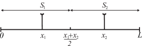
Figure 2: Two base stations competing in a one-dimension space

Definition 1.

The strategic form of the game is given by

$$\mathcal{G}=(\mathcal{K},{\{\mathcal{A}_{k}\}}_{k\in\mathcal{K}},{\{\widehat{U_{k}}\}}_{k\in\mathcal{K}})$$

where

• $\mathcal{K}=\{1,\ldots,K\}$ is the set of players, which are here BS.

• ${\{\mathcal{A}_{k}\}}_{k\in\mathcal{K}}$ is the set of actions players can consider, here

  $$\mathcal{A}_{k}=\{x_{k}\in[0,L]\;|\;0<x_{1}<\ldots<x_{K}<L\}.$$ (10)

  Denote $\mathcal{A}=\{\underline{x}\in[0,L]^{K}\;|\;0<x_{1}<\ldots<x_{K}<L\}$.

• ${\{\widehat{U_{k}}\}}_{k\in\mathcal{K}}$ is the set of utilities players use.

Note that we are interested in location equilibria that do not superimpose several BSs. Thus, if there exists an equilibrium, there exists a spatial order for BSs at this equilibrium, that is why we introduce this order in the action spaces $\{\mathcal{A}_{k}\}_{k\in\mathcal{K}}$.

3 Nash equilibrium analysis

The aim of this section is to show the existence of a Nash equilibrium in the location game described in Section 2.3 and to characterize this equilibrium.

3.1 Existence

In this section, we focus of the existence of a Nash equilibrium in the defined game. To prove the existence of a Nash equilibrium, the concavity of $\widehat{U_{k}}(\underline{x})$ with respect to $x_{k}$ over $\mathcal{A}_{k}$, $\forall k\in\mathcal{K}$, has to be established.

Lemma 1.

$\widehat{U_{k}}(\underline{x})$ is concave with respect to $x_{k}$ over $\mathcal{A}_{k}$, $\forall k\in\mathcal{K}$.

The proof of this lemma is in Appendix A.1. Then one has the following theorem.

Theorem 1.

In the game defined by Definition 1, there exists at least one Nash equilibrium.

Proof.

• Using Lemma 1, we know that $\widehat{U_{k}}\left(\underline{x}\right)$ is concave with respect to $x_{k}$ over $\mathcal{A}_{k}$, $\forall k\in\mathcal{K}$,

• $\widehat{U_{k}}\left(\underline{x}\right)$ is continuous with respect to $\underline{x}$ over $\mathcal{A}$, $\forall k\in\mathcal{K}$,

• the set of feasible actions is compact and convex for all players in the game.

The Rosen [13] conditions for the existence of a Nash equilibrium are met and Theorem  1 is thus proved. ∎

3.2 Multiplicity of NE

Regarding to the uniqueness of the Nash equilibrium, as the characteristics of the BSs (height and noise) are assumed to be identical, it is interesting to note that permuting the order of BSs leads to a symmetric system of equation. Thus, without condition on the order of BSs as in (10), there are $K!$ Nash equilibria for the game and all these equilibria are symmetric, meaning that the set of locations at equilibrium is unique. However, if one imposes the condition order (10), the NE can be shown to be unique by using the Diagonally Strict Concavity (DSC) condition [13].

Theorem 2.

In the game defined by Definition 1, there exists one single Nash equilibrium.

The proof of this theorem is in Appendix A.2. Having uniqueness under this order condition might seem to be a weak result in comparison with a general uniqueness result. However, in the framework of a dynamic process, the initial locations of the base station might suffice to determine the effectively observed NE (after convergence).

3.3 Determination of the NE

A characterization of the equilibrium is provided in this section with examples for small values of $K$. A real solution $\underline{x}$ for $\alpha>2$ has to satisfy

$$\left\{\begin{array}[]{l}x_{1}=\frac{2\sqrt{(5.2^{\frac{2}{\alpha}}-2^{\frac{4}{\alpha}}-4)\varepsilon^{2}+2^{\frac{2}{\alpha}}x_{2}^{2}}-2^{\frac{2}{\alpha}}x_{2}}{4-2^{\frac{2}{\alpha}}},\\ x_{k}=\frac{x_{k+1}+x_{k-1}}{2},\;\forall k\in\{2,\ldots,K-1\},\\ x_{K}=\frac{-2\sqrt{(5.2^{\frac{2}{\alpha}}-2^{\frac{4}{\alpha}}-4)\varepsilon^{2}+2^{\frac{2}{\alpha}}(L-x_{K-1})^{2}}-2^{\frac{2}{\alpha}}x_{K-1}+4L}{4-2^{\frac{2}{\alpha}}}.\end{array}\right.$$ (11)

See Appendix A.3 for detailed derivations. In the case $\alpha=2$, one obtains

$$\left\{\begin{array}[]{l}x_{1}=\sqrt{2\varepsilon^{2}+2x_{2}^{2}}-x_{2},\\ x_{k}=\frac{x_{k+1}+x_{k-1}}{2},\;\forall k\in\{2,\ldots,K-1\},\\ x_{K}=-\sqrt{10\varepsilon^{2}+2(L-x_{K-1})^{2}}-x_{K-1}+2L.\end{array}\right.$$ (12)

In the $2$-player game with $\alpha=2$, one gets

$$\left\{\begin{array}[]{l}x_{1}^{\text{ne}}=L-\frac{1}{2}\sqrt{2L^{2}-4\varepsilon^{2}}\\ x_{2}^{\text{ne}}=\frac{1}{2}\sqrt{2L^{2}-4\varepsilon^{2}}\end{array}\right.$$ (13)

Figure 3 illustrates equilibria for $\alpha=2$ and $\alpha=3$ for respectively two, three, and four BSs.

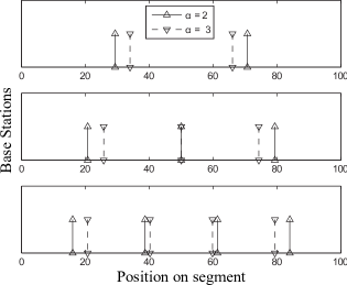
Figure 3: Base Stations at Nash equilibrium for $\alpha=3$ (dotted line) and $\alpha=2$ (continuous line). From the top to the bottom, configuration with 2 BSs, 3 BSs and 4 BSs. Parameters are $\varepsilon=0.1$ and $L=100$.

4 Comparing equilibria

This section compares the Nash equilibrium described in Section 3, the Stackelberg equilibrium, and the social optimum.

4.1 Stackelberg equilibrium

As written in Section 3, the pure Nash equilibrium needs the players to know their spatial order to be reached. If players do not know this order but play in a chronological order, the problem changes. If the first player plays alone at the first stage of the game knowing that other players will place their BSs after, it turns into a Stackelberg game [15] with the first player being the leader of the game. This idea is illustrated with a two-player game with one leader (BS $1$) and one follower (BS $2$). The leader chooses its position knowing that the follower will place itself after. Both BSs still want to maximize their utilities and BS $1$ knows this point. Then, BS $1$ knows how BS $2$ is going to be placed regarding to its own position, it is simply the best response of BS $2$

$$x_{2}(x_{1})=\frac{-2\sqrt{(5.2^{\frac{2}{\alpha}}-2^{\frac{4}{\alpha}}-4)\varepsilon^{2}+2^{\frac{2}{\alpha}}(L-x_{1})^{2}}-2^{\frac{2}{\alpha}}x_{1}+4L}{4-2^{\frac{2}{\alpha}}}.$$

Then BS $1$ places itself at a location $x_{1}$ solution of

$$\frac{\partial\widehat{U_{1}}}{\partial x_{1}}(x_{1},x_{2}(x_{1}))=0.$$ (14)

With $\alpha=2$ and neglecting $\varepsilon$ compared to every other lengths of the problem, one gets

$$x_{1}^{\text{se}}=\biggl{(}1-\sqrt{2}+\sqrt{2-\sqrt{2}}\biggr{)}L,$$ (15)

and

$$x_{2}^{\text{se}}=\biggl{(}(\sqrt{2}-1)(1+\sqrt{2-\sqrt{2}})\biggr{)}L.$$ (16)

On Figure 4, we compare the utilities of the leader and the follower of the Stackelberg game versus the utilities of the Nash equilibrium. As we see, the leader of the Stackelberg game has a better utility than what he would have get at the Nash equilibrium. On the contrary, the follower has a worst utility. Hence, in a mobile operator point of view, it is more interesting to deploy its BS first.

Figure 4: $\frac{\widehat{U_{1}}^{\text{SE}}}{\widehat{U_{1}}^{\text{NE}}}$ and $\frac{\widehat{U_{2}}^{\text{SE}}}{\widehat{U_{2}}^{\text{NE}}}$ with regard to $\varepsilon$.

4.2 Social optimum

Sections 3 and 4.1 provide equilibria corresponding to situations where the BSs only consider what is best for themselves. But these equilibria are not the best for the MTs. In the MTs point-of-view, the utility to consider is the complete utility sum or social utility. In a $2$-BS case

$$\widehat{U}^{\text{so}}\left(x_{1},x_{2}\right)=\widehat{U_{1}}\left(x_{1},x_{2}\right)+\widehat{U_{2}}\left(x_{1},x_{2}\right).$$ (17)

For this utility, we know that there exists an optimum since the strategy set $\mathcal{A}$ is compact and $\widehat{U_{1}}\left(x_{1},x_{2}\right)+\widehat{U_{2}}\left(x_{1},x_{2}\right)$ is continuous with respect to $(x_{1},x_{2})$ over $\mathcal{A}$. At this optimum, it is proven [1] that

• $(i)$ the BSs place themselves at the middle of their associated subset of segment (respectively $\mathcal{S}_{1}$ and $\mathcal{S}_{2}$),

• $(ii)$ the frontier between the two BSs is the middle of the segment.

Thus, we have the optimum

$$x_{1}^{\text{so}}=\frac{L}{4}\mbox{, }x_{2}^{\text{so}}=\frac{3L}{4}.$$ (18)

Figure 5 shows the Nash equilibrium, the Stackelberg equilibrium, and the social optimum for $\alpha=2$. The locations of BSs for Nash equilibrium and social optimum are symmetric with respect to the middle of the segment $\left[0,L\right]$ whereas this is not the case for the Stackelberg equilibrium.

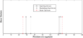
Figure 5: Nash Equilibrium, Stackelberg Equilibrium, and Social Optimum for $\alpha=2$.

4.3 Price of anarchy

To compare the Nash and the Stackelberg equilibrium in the two-player case, we look at the utilities at equilibrium. Without any pricing mechanism, the Nash equilibrium and the social optimum are very close in terms of locations. As a result, they are also close in terms of utility sum. The Price of Anarchy (PoA), introduced in [9], is an adequate metric to compare these sums

$$PoA(eq)=\frac{\max_{\underline{x}\in\mathcal{A}}\sum_{k\in\mathcal{K}}\widehat{U}_{k}(\underline{x})}{\sum_{k\in\mathcal{K}}\widehat{U}_{k}(\underline{x}^{\text{eq}})}.$$ (19)

Note that the PoA is always stronger than $1$ and if the PoA is high, it means that the corresponding equilibrium is not that efficient in terms of utility sum. On the contrary, if the Po1 is close to one, the corresponding equilibrium is satisfying. Figure 6 illustrates the behavior of the PoA for the Nash equilibrium and the PoA for the Stackelberg equilibrium as a function of $\varepsilon$ for $2$-player case. It appears that the Stackelberg equilibrium is less efficient than the Nash equilibrium.

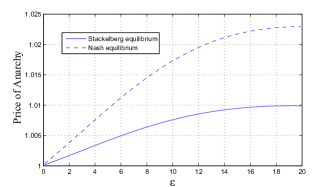
Figure 6: Prices of Anarchy regarding to $\varepsilon$. Parameters are $L=100$, $\sigma^{2}=10^{4}$, $\alpha=2$.

5 Convergence to the Nash equilibrium

Getting to the equilibrium given in Section 3.3 is not simple: it would require that every player knows the utilities of other players. In practice, this is hardly the case. Thus, we present techniques that enable to reach the Nash equilibrium in a decentralized way: best-response dynamics and reinforcement learning. However the BSs need to be movable to perform these two techniques, hence it is more accurate to talk about Mobile Stations (MSs) in the present section. Note that for these two techniques, the only assumption about MSs location is that they cannot superimpose.

5.1 Best response dynamics

The context of this section remains the same as defined in Section 2.3.

The principle of best-response dynamics is that given a realization of actions for its opponents, every player of the game is able to compare its own possible actions and choose which one is best for itself. Precisely the best-response algorithm is the following

1. At every time step $t$, each MS $k$ chooses its location $x^{\text{br}}_{k}(t)$ according to

   $$x^{\text{br}}_{k}(t)=\arg\max_{x_{k}}\,\hat{U}_{k}(x_{k},\underline{x}_{-k}(t)).$$

2. Algorithm stops when $\left|\underline{x}^{\text{br}}(t+1)-\underline{x}^{\text{br}}(t)\right|<\beta$, with $\beta$ fixed.

Regarding to the convergence of this algorithm, we study the system of best-responses (11). If we neglect $\varepsilon$ regarding to $x_{1}$ and $L-x_{K-1}$, one gets a linear system of equations

$$\left\{\begin{array}[]{l}x_{1}=\frac{2^{\frac{1+\alpha}{\alpha}}-2^{\frac{2}{\alpha}}}{4-2^{\frac{2}{\alpha}}}x_{2},\\ x_{k}=\frac{x_{k+1}+x_{k-1}}{2},\;\forall k\in\{2,\ldots,K-1\},\\ x_{K}=\frac{(4-2^{\frac{1+\alpha}{\alpha}})L}{4-2^{\frac{2}{\alpha}}}+\frac{2^{\frac{1+\alpha}{\alpha}}-2^{\frac{2}{\alpha}}}{4-2^{\frac{2}{\alpha}}}x_{K-1}.\end{array}\right.$$ (20)

It is a linear Cournot oligopoly [4].

One distinguishes two ways this algorithm can run.

Simultaneous best response dynamics. At every step, every MS adapt their locations simultaneously. In this case, the evolution of the locations with the algorithm can be expressed by

$$\underline{x}^{\text{br}}(t+1)=\underline{a}+\text{A}_{K}\underline{x}^{\text{br}}(t)$$ (21)

with $\underline{a}=~{}^{t}\bigl{(}0,\ldots,0,\frac{(4-2^{\frac{1+\alpha}{\alpha}})L}{4-2^{\frac{2}{\alpha}}}\bigg{)}$ and

$$\text{A}_{K}=\begin{pmatrix}0&g(\alpha)&0&{3}&0\\ \frac{1}{2}&0&\frac{1}{2}&\ddots&\;&\;&\vdots\\ 0&\ddots&\ddots&\ddots&\ddots&\;&\vdots\\ \vdots&\ddots&\ddots&\ddots&\ddots&\ddots&\vdots\\ \vdots&\;&\ddots&\ddots&\ddots&\ddots&0\\ \vdots&\;&\;&\ddots&\frac{1}{2}&0&\frac{1}{2}\\ 0&{3}&0&g(\alpha)&0\end{pmatrix},$$ (22)

with $g(\alpha)=\frac{2^{\frac{1+\alpha}{\alpha}}-2^{\frac{2}{\alpha}}}{4-2^{\frac{2}{\alpha}}}$.

As recalled in Lemma 2.8 of [16], for an irreducible positive square matrix A$=(a_{ij})_{1\leq i\leq n}$, then either

$$\sum_{j=1}^{n}{a_{ij}}=\rho(\text{A})\;\forall i\in[1,n],$$ (23)

or

$$\inf_{1\leq i\leq n}\sum_{j=1}^{n}{a_{ij}}<\rho(\text{A})<\sup_{1\leq i\leq K}\sum_{j=1}^{n}{a_{ij}},$$ (24)

with $\rho(\text{A})$ being the radius of A. In our case, $\text{A}_{K}$ can be verified to be positive and irreducible, then one has

$$g(\alpha)<\rho(\text{A}_{K})<1.$$ (25)

Hence, the convergence of the algorithm is ensured.

Sequential best response dynamics. The other case is the sequential algorithm: at every step, only one MS adapts its location. Depending on the MS $k$ adapting its location, the algorithm evolves according to

$$\underline{x}^{\text{br}}(t+1)=\underline{a}+\text{A}^{k}_{K}\underline{x}^{\text{br}}(t),$$ (26)

with $\text{A}^{k}_{K}$ corresponding to the adaptation of the $k$-th MS. $\text{A}^{k}_{K}$ may have several forms.

• If the $k$-th MS, $k\in\{2,\ldots,K-1\}$ adapts its location, then

  $$\text{A}^{k}_{K}=\begin{pmatrix}1&0&{4}&0\\ \ddots&\ddots&\ddots&\;&\;&\;&\vdots\\ \vdots&0&1&0&\;&\;&\vdots\\ \vdots&\;&\frac{1}{2}&0&\frac{1}{2}&\;&\vdots\\ \vdots&\;&\;&0&1&0&\vdots\\ \vdots&\;&\;&\;&\ddots&\ddots&\ddots\\ 0&{4}&0&1\end{pmatrix}$$

  In this case, $\text{A}^{k}_{K}$ is irreducible and positive and

  $$\rho(\text{A}^{k}_{K})=1.$$ (27)

• If the first MS adapts its location, the matrix has the form

  $$\text{A}^{1}_{K}=\begin{pmatrix}0&g(\alpha)&0&\ldots\\ 0&1&0&\;\\ \vdots&\ddots&\ddots&\ddots\\ 0&\ldots&0&1\end{pmatrix}$$

  Again, $\text{A}^{1}_{K}$ is irreducible and positive, but this time

  $$g(\alpha)<\rho(\text{A}^{1}_{K})<1.$$ (28)

  Note that if the $K$-th MS adapts its location, the same reasoning can be done.

  $$g(\alpha)<\rho(\text{A}^{K}_{K})<1.$$ (29)

Hence, $\rho(\prod_{k=1}^{K}{\text{A}^{k}_{K}})=\prod_{k=1}^{K}{\rho(\text{A}^{k}_{K})}<1$ and the algorithm converges.

In Figure 7, we compare MSs $1$ and $2$ sequential best-responses for $\alpha=2$.

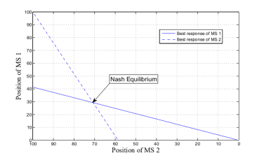
Figure 7: Best-responses of MS $1$ and MS $2$ for $\alpha=2$

5.2 Reinforcement Learning

The following notations are used in this section. For a set of MSs $\mathcal{K}=\{1,\ldots,K\}$, let $\mathcal{\tilde{A}}_{k}=\{y_{k1},\ldots,y_{km_{k}}\}$ be the set of possible locations for MS $k$ ($m_{k}$ being the cardinality of $\mathcal{\tilde{A}}_{k}$), which corresponds to a discretization of the set $\left[0,L\right]$.

We implement a discrete stochastic learning algorithm in the sense that the action space is discrete and at every step, actions are chosen in a stochastic way. The only information available to a MS is the value of its utility after each iteration (note that the MS does not necessarily knows its utility expression).

We define $\underline{p}_{k}(t)=(p_{k1}(t),\ldots,p_{km_{k}}(t))$ the probability distribution vector of MS $k$ at time $t$.

$$\text{P}\left[x_{k}(t)=y_{ki}\right]=p_{ki}(t),\;i\in\{1,\ldots,m_{k}\}.$$ (30)

The algorithm used by each MS is then the following.

1. Initialize the distribution probability vector.

   $\forall k\in\mathcal{K},\;\forall i\in\{1,\ldots,m_{k}\},\;p_{ki}(0)=\frac{1}{m_{k}}.$

2. At every step $t$, each MS $k$ chooses a location $x_{k}(t)$ according to its probability vector $\underline{p}_{k}(t)$.

3. Each MS gets $U_{k}(t)$.

4. Each MS updates its probability distribution vector $\underline{p}_{k}(t)$

   $$\begin{array}[]{ll}p_{ki}(t+1)=p_{ki}(t)-bU_{k}(t)p_{ki}(t)\text{, if }x_{t}(t)\neq y_{ki}&\\ p_{ki}(t+1)=p_{ki}(t)+bU_{k}(t)\sum_{s\neq i}{p_{k}s}(t)\text{, if }x_{k}(t)=y_{ki}&\end{array}$$ (31)

5. Algorithm stops when $\underline{p}_{k}(t+1)=\underline{p}_{k}(t)$, else go to step $2$.

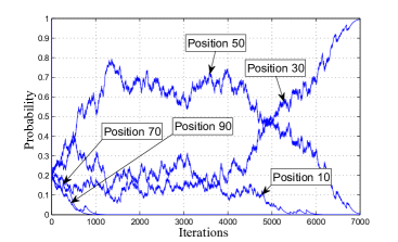
Figure 8: Evolution of action probabilities for BS 1 with discrete stochastic learning.

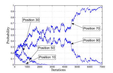
Figure 9: Evolution of action probabilities for BS 2 with discrete stochastic learning.

Figures 8 and 9 illustrate the evolution of the probability distribution vectors of two MSs. The parameters of the simulation are the following: each MS has the same set of possible positions $\{10,30,50,70,90\}$ and the step of the learning algorithm is $b=0.01$.

Depending on the choice of $b$, two phenomena occur.

• The higher the value of $b$, the lower the convergence time of the algorithm,

• However, if $b$ is chosen too high, the algorithm may converge to locations that do no correspond to an equilibrium of the game defined in Section 2.3.

Figure 10 illustrates the convergence time as a function of $b$.

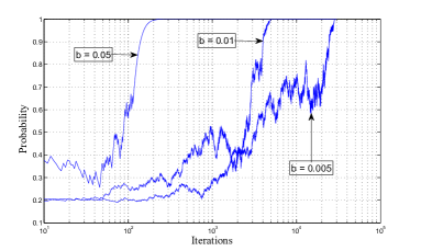
Figure 10: Convergence of probability with respect to step $b$

The choice of $b$ is hence a trade-off between convergence time and accuracy of the convergence.

6 Conclusion and perspectives

Obviously the proposed model is relatively simple and should be improved to obtain refined results. However, this led us to several interesting results such as a full characterization of Nash equilibria and interesting behavior in terms of convergence. It would be very relevant to extend this work to two-dimensional scenario, define a suitable order for which uniqueness would be ensured. More connections with the famous multi-source Weber problem [6] should be established to better understand the general problem of deployment games. Indeed, if an operator has to locate a set of base stations, the problem becomes more complicated. The problem becomes even more interesting if the set of possible constellations is discrete, which would lead us to make connections with Voronoi games [5]. The authors believe there is large avenue for contributions to the general problem under study, especially in finding relevant assumptions to simplify it without too loss in terms of understanding. Random matrix theory and stochastic geometry might be for great help to achieve this challenging objective.

Appendix A Proofs

A.1 Proof of Lemma 1

We need to prove that $\widehat{U_{k}}(\underline{x})$ is concave with respect to $x_{k}$ over $\mathcal{A}_{k}$.

We know that the index of players verify $\left(\ref{eq:order}\right)$. In this case, the regions associated to the BSs are

$$\left\{\begin{array}[]{l}\text{[}0,\frac{x_{1}+x_{2}}{2}\text{] for BS $1,$}\\ \text{[}\frac{x_{k-1}+x_{k}}{2},\frac{x_{k}+x_{k+1}}{2}\text{]}\text{ for BS $k$, }k\in\{2,\ldots,K-1\}\\ \text{[}\frac{x_{K-1}+x_{K}}{2},L\text{]}\text{ for BS $K.$}\end{array}\right.$$ (32)

Then

$$\left\{\begin{array}[]{l}\widehat{U_{1}}(\underline{x})=\int_{0}^{\frac{x_{1}+x_{2}}{2}}(\varepsilon^{2}+(x-x_{1})^{2})^{-\frac{\alpha}{2}}{\text{d}x}\\ \widehat{U_{k}}(\underline{x})=\int_{\frac{x_{k-1}+x_{k}}{2}}^{\frac{x_{k}+x_{k+1}}{2}}(\varepsilon^{2}+(x-x_{k})^{2})^{-\frac{\alpha}{2}}{\text{d}x},\;k\in\{2,\ldots,K-1\}\\ \widehat{U_{K}}(\underline{x})=\int_{\frac{x_{K-1}+x_{K}}{2}}^{L}(\varepsilon^{2}+(x-x_{K})^{2})^{-\frac{\alpha}{2}}{\text{d}x}\end{array}\right.$$ (33)

which may be rewritten as

$$\left\{\begin{array}[]{lll}\widehat{U_{1}}(\underline{x})=\int_{-x_{1}}^{\frac{x_{2}-x_{1}}{2}}(\varepsilon^{2}+x^{2})^{-\frac{\alpha}{2}}{\text{d}x}&&\\ \widehat{U_{k}}(\underline{x})=\int_{\frac{x_{k-1}-x_{k}}{2}}^{\frac{x_{k+1}-x_{k}}{2}}(\varepsilon^{2}+x^{2})^{-\frac{\alpha}{2}}{\text{d}x},\;k\in\{2,\ldots,K-1\}&&\\ \widehat{U_{K}}(\underline{x})=\int_{\frac{x_{K-1}-x_{K}}{2}}^{L-x_{K}}(\varepsilon^{2}+x^{2})^{-\frac{\alpha}{2}}{\text{d}x}&&\end{array}\right.$$ (34)

To prove the existence of a Nash equilibrium, the concavity of $\widehat{U_{k}}\left(\underline{x}\right)$ with respect to $x_{k}$ $\forall k\in\mathcal{K}$ has now to be established. One has the first-order partial derivatives

$$\left\{\begin{array}[]{l}\frac{\partial\widehat{U_{1}}}{\partial x_{1}}(\underline{x})=-\frac{1}{2}(\varepsilon^{2}+(\frac{x_{2}-x_{1}}{2})^{2})^{-\frac{\alpha}{2}}+(\varepsilon^{2}+x_{1}^{2})^{-\frac{\alpha}{2}}\\ \frac{\partial\widehat{U_{k}}}{\partial x_{k}}(\underline{x})=-\frac{1}{2}(\varepsilon^{2}+(\frac{x_{k+1}-x_{k}}{2})^{2})^{-\frac{\alpha}{2}}+\frac{1}{2}(\varepsilon^{2}+(\frac{x_{k-1}-x_{k}}{2})^{2})^{-\frac{\alpha}{2}}\\ \frac{\partial\widehat{U_{K}}}{\partial x_{K}}(\underline{x})=-(\varepsilon^{2}+(L-x_{K})^{2})^{-\frac{\alpha}{2}}+\frac{1}{2}(\varepsilon^{2}+(\frac{x_{K-1}-x_{K}}{2})^{2})^{-\frac{\alpha}{2}}\end{array}\right.$$ (35)

and the second-order partial derivatives

$$\left\{\begin{array}[]{l}\frac{\partial^{2}\widehat{U_{1}}}{\partial x_{1}^{2}}(\underline{x})=-\frac{\alpha}{8}\frac{x_{2}-x_{1}}{(\varepsilon^{2}+(\frac{x_{2}-x_{1}}{2})^{2})^{\frac{\alpha}{2}+1}}-\alpha\frac{x_{1}}{(\varepsilon^{2}+x_{1}^{2})^{\frac{\alpha}{2}+1}}\\ \frac{\partial^{2}\widehat{U_{k}}}{\partial x_{k}^{2}}(\underline{x})=\frac{\alpha}{8}\bigl{(}-\frac{x_{k+1}-x_{k}}{(\varepsilon^{2}+(\frac{x_{k+1}-x_{k}}{2})^{2})^{\frac{\alpha}{2}+1}}+\frac{x_{k-1}-x_{k}}{(\varepsilon^{2}+(\frac{x_{k-1}-x_{k}}{2})^{2})^{\frac{\alpha}{2}+1}}\bigr{)}\\ \frac{\partial^{2}\widehat{U_{K}}}{\partial x_{K}^{2}}(\underline{x})=-\alpha\frac{L-x_{K}}{(\varepsilon^{2}+(L-x_{K})^{2})^{\frac{\alpha}{2}+1}}+\frac{\alpha}{8}\frac{x_{K-1}-x_{K}}{(\varepsilon^{2}+(\frac{x_{K-1}-x_{K}}{2})^{2})^{\frac{\alpha}{2}+1}}\end{array}\right.$$ (36)

Given $\left(\ref{eq:order}\right)$, we have $\frac{\partial^{2}\widehat{U_{k}}}{\partial x_{k}^{2}}(\underline{x})<0\;\forall k\in\mathcal{K}$. Thus $\widehat{U_{k}}(\underline{x})$ is concave with respect to $x_{k}$ over$\mathcal{A}_{k}$, $\forall k\in\mathcal{K}$.

A.2 Proof of Theorem 2

In the context of $K$-player game, the DSC [13] condition writes $\forall(\underline{a},\underline{a}^{\prime})\in\mathcal{A}^{2}$ such that $\underline{a}\neq\underline{a}^{\prime}$

$$\sum_{k=1}^{K}(a^{\prime}_{k}-a_{k})\biggl{(}\frac{\partial\widehat{U_{k}}}{\partial x_{k}}(\underline{a})-\frac{\partial\widehat{U_{k}}}{\partial x_{k}}(\underline{a}^{\prime})\biggr{)}>0$$ (37)

For clarity reasons, we denote

$$g(a,b)=\biggl{(}(\epsilon^{2}+a^{2})^{-\frac{\alpha}{2}}-(\epsilon^{2}+b^{2})^{-\frac{\alpha}{2}}\biggr{)},\;(a,b)\in\mathbb{R}^{2}.$$ (38)

By (35), it turns

$$\left\{\begin{array}[]{l}\scriptstyle{\frac{\partial\widehat{U_{1}}}{\partial x_{1}}(\underline{a})-\frac{\partial\widehat{U_{1}}}{\partial x_{1}}(\underline{a}^{\prime})=g(a_{1},a^{\prime}_{1})-\frac{1}{2}\biggl{(}g(\frac{a_{1}-a_{2}}{2},\frac{a^{\prime}_{1}-a^{\prime}_{2}}{2})\biggr{)}}\\ \scriptstyle{\frac{\partial\widehat{U_{k}}}{\partial x_{k}}(\underline{a})-\frac{\partial\widehat{U_{k}}}{\partial x_{k}}(\underline{a}^{\prime})=\frac{1}{2}\biggl{(}g(\frac{a_{k-1}-a_{k}}{2},\frac{a^{\prime}_{k-1}-a^{\prime}_{k}}{2})-g(\frac{a_{k}-a_{k+1}}{2},\frac{a^{\prime}_{k}-a^{\prime}_{k+1}}{2})\biggr{)}}\\ \scriptstyle{\frac{\partial\widehat{U_{K}}}{\partial x_{K}}(\underline{a})-\frac{\partial\widehat{U_{K}}}{\partial x_{K}}(\underline{a}^{\prime})=\frac{1}{2}\biggl{(}g(\frac{a_{K-1}-a_{K}}{2},\frac{a^{\prime}_{K-1}-a^{\prime}_{k}}{2})\biggr{)}-g(L-a_{K},L-a^{\prime}_{K})}\end{array}\right.$$ (39)

Equation (37) becomes

$$\scriptstyle{(a^{\prime}_{1}-a_{1})\biggl{(}g(a_{1},a^{\prime}_{1})-\frac{1}{2}g(\frac{a_{1}-a_{2}}{2},\frac{a^{\prime}_{1}-a^{\prime}_{2}}{2})\biggr{)}}$$ (40)

$$\scriptstyle{+\sum_{k=2}^{K-1}\frac{a^{\prime}_{k}-a_{k}}{2}\biggl{(}g(\frac{a_{k-1}-a_{i}}{2},\frac{a^{\prime}_{k-1}-a^{\prime}_{k}}{2})-g(\frac{a_{k}-a_{k+1}}{2},\frac{a^{\prime}_{k}-a^{\prime}_{k+1}}{2})\biggr{)}}$$

$$\scriptstyle{+(a^{\prime}_{K}-a_{K})\biggl{(}\frac{1}{2}g(\frac{a_{K-1}-a_{K}}{2},\frac{a^{\prime}_{K-1}-a^{\prime}_{K}}{2})-g(L-a_{K},L-a^{\prime}_{K})\biggr{)}>0}$$

which can also be written

$$(a^{\prime}_{1}-a_{1})g(a_{1},a^{\prime}_{1})$$ (41)

$$+\sum_{k=2}^{K}\frac{a^{\prime}_{k}-a^{\prime}_{k-1}-(a_{k}-a_{k-1})}{2}g\biggl{(}\frac{a_{k-1}-a_{k}}{2},\frac{a^{\prime}_{k-1}-a^{\prime}_{k}}{2}\biggr{)}$$

$$+(L-a^{\prime}_{K}-(L-a_{K}))g(L-a_{K},L-a^{\prime}_{K})>0$$

However $\forall(a,b)\in\mathbb{R}^{*2}$,

$$(b-a)g(a,b)>0$$ (42)

and by the order condition (10)

$$\left\{\begin{array}[]{lll}(a^{\prime}_{1},a_{1})\in\mathbb{R}^{*2}\\ (\frac{a^{\prime}_{k}-a^{\prime}_{k-1}}{2},\frac{a_{k}-a_{k-1}}{2})\in\mathbb{R}^{*2}\;\forall k\in\{2,\ldots,K\}\\ (L-a^{\prime}_{K},L-a_{K})\in\mathbb{R}^{*2}\end{array}\right.$$ (43)

Then the DSC condition is verified and the equilibrium is unique.

A.3 Derivation of (11)

To obtain a formal expression of a Nash equilibrium, the intersection of the best-responses has to be considered

$$\frac{\partial\hat{U}_{k}}{\partial x_{k}}(\underline{x})=0,\;\forall k\in\mathcal{K},\;\forall\alpha\geqslant 2.$$ (44)

$\left(\ref{Eq:BestRespInter}\right)$ leads to

$$\left\{\begin{array}[]{l}(2^{\frac{2}{\alpha}}(\varepsilon^{2}+(\frac{x_{2}-x_{1}}{2})^{2}))^{\frac{\alpha}{2}}=(\varepsilon^{2}+x_{1}^{2})^{\frac{\alpha}{2}}\\ (\varepsilon^{2}+(\frac{x_{k+1}-x_{k}}{2})^{2})^{\frac{\alpha}{2}}=(\varepsilon^{2}+(\frac{x_{k-1}-x_{k}}{2})^{2})^{\frac{\alpha}{2}},\;\forall k\in\{2,\ldots,K-1\}\\ (\varepsilon^{2}+(L-x_{K})^{2})^{\frac{\alpha}{2}}=(2^{\frac{2}{\alpha}}(\varepsilon^{2}+(\frac{x_{K-1}-x_{K}}{2})^{2}))^{\frac{\alpha}{2}}.\end{array}\right.$$ (45)

Since all terms elevated at power $\alpha/2$ are positive, one gets

$$\left\{\begin{array}[]{l}2^{\frac{2}{\alpha}}(\varepsilon^{2}+(\frac{x_{2}-x_{1}}{2})^{2})=\varepsilon^{2}+x_{1}^{2}\\ (\frac{x_{i+k}-x_{k}}{2})^{2}=(\frac{x_{k-1}-x_{k}}{2})^{2},\;\forall k\in\{2,\ldots,K-1\}\\ 2^{\frac{2}{\alpha}}(\varepsilon^{2}+(\frac{x_{K-1}-x_{K}}{2})^{2})=\varepsilon^{2}+(L-x_{K})^{2}\end{array}\right.$$ (46)

One real solution $\underline{x}$ verifying $\left(\ref{eq:order}\right)$ has thus to satisfy $\left(\ref{eq:charac}\right)$ when$\,\alpha>2$ and $\left(\ref{eq:charac2}\right)$ when $\alpha=2$.

References

- [1] Eitan Altman, Anurag Kumar, Chandramani Kishore Singh, and Rajesh Sundaresan. Spatial sinr games combining base station placement and mobile association. In INFOCOM, pages 1629–1637. IEEE, 2009.
- [2] Eitan Altman, Alonso Silva, Amidou Tembine, and Merouane Debbah. Spatial games and global optimization for the mobile association problem: the downlink case. In IEEE/SIAM CDC’, 2010.
- [3] Robert R. Bush and Frederick Mosteller. Stochastic Models for Learning. Wiley, 1st edition, 1955.
- [4] A. Cournot. Researches into the principles of wealth. Irwin Paperback Classics in Economics (original: Recherches sur les principes mathématiques de la théorie des richesses, 1838), 1963 (English Translation).
- [5] Christoph Dürr and Nguyen Kim Thang. Nash equilibria in Voronoi games on graphs. CoRR, abs/cs/0702054, 2007.
- [6] Sándor P. Fekete, Joseph S. B. Mitchell, and Karin Beurer. On the continuous fermat-weber problem. CoRR, cs.CG/0310027, 2003.
- [7] Jean J. Gabszewicz and Jacques-Francois Thisse. Location. In R.J. Aumann and S. Hart, editors, Handbook of Game Theory with Economic Applications, volume 1 of Handbook of Game Theory with Economic Applications, chapter 9, pages 281–304. Elsevier, 1992.
- [8] Harold Hotelling. Stability in competition. The Economic Journal, 39(153):41–57, 1929.
- [9] Elias Koutsoupias and Christos Papadimitriou. Worst-case equilibria. In the 16th Annual Symposium on Theoretical Aspects of Computer Science, pages 404–413, 1999.
- [10] John Litva and Titus K. Lo. Digital Beamforming in Wireless Communications. Artech House, Inc., Norwood, MA, USA, 1996.
- [11] Kumpati S. Narendra and Mandayam A. L. Thathachar. Learning automata: an introduction. Prentice-Hall, Inc., Upper Saddle River, NJ, USA, 1989.
- [12] Frank Plastria. Static competitive facility location: An overview of optimisation approaches. European Journal of Operational Research, 129(3):461–470, March 2001.
- [13] J. B. Rosen. Existence and Uniqueness of Equilibrium Points for Concave N-Person Games. Econometrica, 33(3):520–534, 1965.
- [14] P.S. Sastry, V.V. Phansalkar, and M.A.L. Thathachar. Decentralized learning of nash equilibria in multi-person stochastic games with incomplete information. Systems, Man and Cybernetics, IEEE Transactions on, 24(5):769 –777, May 1994.
- [15] H. Stackelberg. Marketform und Gleichgewicht. Oxford, U.K., 1934.
- [16] Richard S. Varga. Matrix iterative analysis. Springer series in computational mathematics, 27. Springer, 2nd rev. and expanded ed. edition, 2000.