Role of the on-site pinning potential in establishing quasi-steady-state conditions of heat transport in finite quantum systems

Abstract

We study the transport of energy in a finite linear harmonic chain by solving the Heisenberg equation of motion, as well as by using nonequilibrium Green’s functions to verify our results. The initial state of the system consists of two separate and finite linear chains that are in their respective equilibriums at different temperatures. The chains are then abruptly attached to form a composite chain. The time evolution of the current from just after switch-on to the transient regime and then to later times is determined numerically. We expect the current to approach a steady-state value at later times. Surprisingly, this is possible only if a nonzero quadratic on-site pinning potential is applied to each particle in the chain. If there is no on-site potential a recurrent phenomenon appears when the time scale is longer than the traveling time of sound to make a round trip from the midpoint to a chain edge and then back. Analytic expressions for the transient and steady-state currents are derived to further elucidate the role of the on-site potential.

I Introduction

In the study of thermal transport in quantum systems, the conventional setup examined is a scattering region sandwiched between two infinite leads acting as large heat reservoirs wang08 . The leads and the scattering region are initially prepared to be at their respective thermal equilibriums in canonical distributions and then are coupled using an adiabatic switch-on. The long-time steady-state current through the scattering region can be calculated using the Landauer formula where the transmission coefficient can be determined using nonequilibrium Green’s function techniques wang08 . This approach, however, is not applicable to situations where the system is undergoing dynamical changes and is far from the steady-state regime. An example would be the transient behavior of a system where the coupling between the scattering region and the leads is not weak and is switched on abruptly cuansing10 . In addition, the method does not provide any information on how the steady state is dynamically approached from the initial configuration of the system. In this work we examine the time evolution of the thermal current from the transient regime just after an abrupt switch-on to the intermediate-time quasi-steady-state regime and then to the long-time recurrent regime, in a system consisting only of two finite leads that are coupled abruptly at time $t=0$. We examine if, when, and how the onset of the steady-state occurs. To determine the current, we solve the quantum equations of motion of the linear system. In addition, a supplementary second method we employ to verify our results is an approach using nonequilibrium Green’s functions that takes into account the full time evolution of the system cuansing10 .

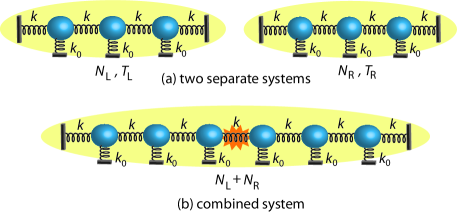
Figure 1: (Color online) An illustration of how two finite independent systems at temperature $T_{\rm L}$ and $T_{\rm R}$, containing $N_{\rm L}$ and $N_{\rm R}$ particles, are abruptly combined at $t=0$ into a composite system containing $N_{\rm L}+N_{\rm R}$ particles. The interparticle spring constant is $k$ and the on-site spring constant is $k_{0}$.

We determine the thermal current in a phonon system consisting of two linear chains abruptly attached together at time $t=0$. Shown in Fig. 1(a) are the two separate linear chains. The interparticle spring constant is $k$ and the on-site spring constant is $k_{0}$. The left and right leads contain $N_{L}$ and $N_{R}$ sites and have temperature $T_{L}$ and $T_{R}$, respectively. The chains are initially in their respective thermal equilibrium; i.e., they are initially attached to heat baths so that they acquire their corresponding temperatures and then the baths are subsequently detached. The chains therefore satisfy canonical distributions. They also follow fixed boundary conditions wherein particles at the left and right edges are attached to fixed walls. At time $t=0$ the chains are abruptly coupled with spring constant $k$, as shown in Fig. 1(b). The composite chain also satisfies fixed boundary conditions. We then determine the energy current flowing through the newly formed interleads coupling. Since the chains are finite, we cannot use the Landauer formula approach to calculate the current. However, results from the Landauer formula can be used for comparison to the infinitely large and long-time limit results of the approaches we describe.

The probability of extracting work in a system that is weakly coupled to finite heat baths is found to follow a power law campisi09 . In this paper, in comparison, we examine the energy current flowing between two finite chains whose coupling is not weak. We find that the presence of a quadratic on-site pinning potential is necessary in establishing a steady-state current. Previous studies have found that the on-site pinning potential plays an important role in how the steady-state phonon current depends on the system size in disordered harmonic systems pinning . In this work we further investigate the role of the on-site potential on the dynamics of the system and find that. without a quadratic on-site pinning potential, the current exhibits oscillatory behavior that does not disappear even for long times. Furthermore, we find that the time period of oscillation of the current is proportional to the sum of the length of the finite chains. Studies in systems consisting of classical harmonic oscillators and classical particles indicate that the Poincaré recurrence time, i.e., the time for a specific phase-space configuration of the system, or a configuration that very closely resembles it, to reappear increases exponentially with the number of degrees of freedom frisch56 ; zwanzig01 . Recurrence of the wave function is also found to occur in quantum systems with discrete energy spectrum bocchieri59 and systems that are periodically driven hogg82 . Our work extends these studies on quantum systems by examining a physical observable, i.e., the energy current, in a finite system to see if it displays recurrent behavior and to determine conditions that dictate the appearance of recurrence. In Sec. IV our results show that the presence of an on-site potential is crucial to determine whether the energy current exhibits a recurrent and oscillatory behavior or a behavior that decays and settles to a quasi-steady-state value.

In electron systems, the transport of electrons between two finite leads has previously been studied bushong05 . When there is a potential bias between the leads, it is found that a quasi-steady-state current with a finite lifetime appears, even when there are no dissipative effects like electron-electron and electron-ion interactions. In this paper, we supplement this electron transport study by examining the transport of phonons within a finite system. We determine the dynamical behavior of the thermal current and find that having on-site pinning potentials is necessary in establishing the quasi-steady-state current.

II The eigenmode approach

We model the left and right chains by the harmonic Hamiltonian

$$H^{\alpha}=\frac{1}{2}(p^{\alpha})^{T}p^{\alpha}+\frac{1}{2}(u^{\alpha})^{T}K^{\alpha}u^{\alpha},~{}~{}~{}\alpha={\rm L,R},$$ (1)

where $u^{\alpha}$ is a column vector whose elements are the renormalized displacements of the sites in chain $\alpha$, $p^{\alpha}$ is the conjugate momentum, and $K^{\alpha}$ is the tridiagonal spring constant matrix consisting of $2k+k_{0}$ along the diagonal and $-k$ along the two off-diagonals. $k$ is the nearest-neighbor spring constant and $k_{0}$ is the spring constant of the on-site pinning potential. The spring potentials we consider in this work are all quadratic. The equations of motion of particles in the left chain are

$$\dot{u}^{\rm L}=p^{\rm L}~{}~{}~{}{\rm and}~{}~{}~{}\ddot{u}^{\rm L}=\dot{p}^{\rm L}=-K^{\rm L}u^{\rm L}-V^{\rm LR}u^{\rm R},$$ (2)

where $V^{\rm LR}$ is the coupling matrix between the left and right chains. Particles in the right chain satisfy a similar set of equations of motion. The current flowing out of the left chain can be calculated from the chain’s average rate of decrease in energy,

$$I^{\rm L}={} -\left<\dot{H}^{\rm L}\right>=\left<p^{\rm L}(t)^{T}~{}V^{\rm LR}~{}u^{\rm R}(t)\right>$$

$$={} \sum_{jk}\left<p_{j}^{\rm L}(t)~{}V_{jk}^{\rm LR}~{}u_{k}^{\rm R}(t)\right>,$$ (3)

where the equations of motion in Eq. (2) are used. The average is taken with respect to the initial product state density matrix. To calculate the energy current out of the left chain, therefore, we need to determine the dynamics of $u^{\rm R}(t)$ and $p^{\rm L}(t)$.

Consider an isolated finite linear chain consisting of $N$ sites and satisfying fixed boundary conditions. Since it is isolated, the equations of motion of its constituent particles are

$$\dot{u}=p~{}~{}~{}{\rm and}~{}~{}~{}\ddot{u}=\dot{p}=-K\,u,$$ (4)

where $K$ is the spring constant matrix of the whole chain. The solution is

$$\begin{split}u(t)&=\cos(\sqrt{K}t)\,u_{0}+\frac{1}{\sqrt{K}}\sin(\sqrt{K}t)\,p_{0},\\ p(t)&=-\sqrt{K}\sin(\sqrt{K}t)\,u_{0}+\cos(\sqrt{K}t)\,p_{0},\end{split}$$ (5)

where $u_{0}$ and $p_{0}$ are determined from the initial condition. Since the system is linear, quantum Heisenberg operators and classical variables have identical solutions. To make the solution numerically amenable, we construct a transformation, using eigenmodes, that diagonalizes the matrix $K$. Let $u^{n}$ be the $n$th eigenmode of $K$, i.e., $K\,u^{n}=\Omega_{n}^{2}\,u^{n}$, where $\Omega_{n}^{2}$ is the eigenvalue associated with $u^{n}$, i.e.,

$$\Omega_{n}^{2}=2k\left(1-\cos q_{n}\right)+k_{0},$$ (6)

where $q_{n}=\pi n/(N+1)$ and $n=1,2,\cdots,N$. Because of the fixed boundary conditions, the $j$th element of the eigenmode is $u_{j}^{n}=A_{n}\,\sin(q_{n}\,j)$, where $A_{n}$ can be fixed by an appropriate normalization. Let $S$ be a matrix consisting of the eigenmodes of $K$, i.e., $S=(u^{1},u^{2},\ldots,u^{N})$. We can then fix $A_{n}$ by normalizing $SS^{T}=S^{T}S=1$. We get

$$A_{n}=\sqrt{\frac{2}{N+1}}.$$ (7)

The matrix $K$ is diagonalized by the similarity transformation

$$S^{T}KS={\rm diag}(\Omega_{1}^{2},\Omega_{2}^{2},\ldots,\Omega_{N}^{2})\equiv\Omega^{2},$$ (8)

where the right-hand side is a diagonal matrix consisting of elements $\Omega_{1}^{2}$, $\Omega_{2}^{2}$, $\ldots$, $\Omega_{N}^{2}$. The coefficients involving $K$ in Eq. (5) can now be calculated with the aid of the above similarity transformation. We are then left with the unknowns $u_{0}$ and $p_{0}$, and their correlations. To determine these unknowns, we write $u_{0}$ in normal mode coordinates, i.e., $u_{0}=SQ$, where $Q$ contains the normal modes. In a harmonic oscillator with Hamiltonian $H_{ho}=\sum_{j}\hbar\Omega_{j}(a_{j}^{\dagger}a_{j}+1/2)$, the $j$th normal mode is

$$\begin{split}Q_{j}&=\sqrt{\frac{\hbar}{2\Omega_{j}}}(a_{j}+a_{j}^{\dagger}),\\ P_{j}&=\dot{Q}_{j}=-i\Omega_{j}\sqrt{\frac{\hbar}{2\Omega_{j}}}(a_{j}-a_{j}^{\dagger}),\end{split}$$ (9)

where $a_{j}(t)=a_{j}(0)e^{-i\Omega_{j}t}$ and its complex conjugate are the time-dependent lowering and raising ladder operators. These ladder operators satisfy expectation values $\left<a_{j}^{\dagger}a_{k}\right>=\delta_{jk}f_{j}$, $\left<a_{j}a_{k}^{\dagger}\right>=\delta_{jk}(f_{j}+1)$, and $\left<a_{j}^{\dagger}a_{k}^{\dagger}\right>=\left<a_{j}a_{k}\right>=0$, where $f_{j}=(\exp(\hbar\Omega_{j}/k_{B}T)-1)^{-1}$ is the Bose-Einstein distribution function. Using these expectation values, we get

$$\begin{split}\left<Q_{j}Q_{k}\right>&=\frac{\hbar}{2\Omega_{j}}\left(2f_{j}+1\right)\delta_{jk},\\ \left<Q_{j}P_{k}\right>&=\frac{i\hbar}{2}\delta_{jk},\\ \left<P_{j}Q_{k}\right>&=-\frac{i\hbar}{2}\delta_{jk},\\ \left<P_{j}P_{k}\right>&=\Omega_{j}\frac{\hbar}{2}\left(2f_{j}+1\right)\delta_{jk}.\end{split}$$ (10)

Using $S$ and the above expectation values, we can write

$$\begin{split}\left<u_{0j}u_{0k}\right>&=\sum_{m}S_{jm}\frac{\hbar}{2\Omega_{m}}\left(2f_{m}+1\right)S_{km},\\ \left<u_{0j}p_{0k}\right>&=\sum_{m}S_{jm}\frac{i\hbar}{2}S_{km},\\ \left<p_{0j}u_{0k}\right>&=-\sum_{m}S_{jm}\frac{i\hbar}{2}S_{km},\\ \left<p_{0j}p_{0k}\right>&=\sum_{m}S_{jm}\frac{\hbar}{2}\left(2f_{m}+1\right)\Omega_{m}S_{km}.\end{split}$$ (11)

For the composite chain in Fig. 1(b), we label the sites consecutively from $1$ for the leftmost site to $N_{\rm L}+N_{\rm R}$ for the rightmost site. Thus, the labels of the sites where the newly formed interleads spring appears are $N_{\rm L}$ and $N_{\rm L}+1$. In Eq. (3) therefore, the indices are $j=N_{\rm L}$ and $k=N_{\rm L}+1$. The expectation value in Eq. (3), using the solutions in Eq. (5), can then be written as

$$\left<p_{N_{\rm L}}^{\rm L}(t)\,u_{N_{\rm L}+1}^{\rm R}(t)\right>=\sum_{j,k=1}^{N_{\rm L}}\Upsilon_{jk}^{\rm L}+\sum_{j,k=N_{\rm L}+1}^{N_{\rm L}+N_{\rm R}}\Upsilon_{jk}^{\rm R},$$ (12)

where

$$\begin{split}\Upsilon_{jk}^{\alpha}&=C_{j}\,A_{k}\left<u_{0j}^{\alpha}u_{0k}^{\alpha}\right>+C_{j}\,B_{k}\left<u_{0j}^{\alpha}p_{0k}^{\alpha}\right>\\ &+D_{j}\,A_{k}\left<p_{0j}^{\alpha}u_{0k}^{\alpha}\right>+D_{j}\,B_{k}\left<p_{0j}^{\alpha}p_{0k}^{\alpha}\right>,\end{split}$$ (13)

and $\alpha={\rm L,R}$. The $\left<up\right>$ and $\left<pu\right>$ terms cancel exactly and only the $\left<uu\right>$ and $\left<pp\right>$ correlations contribute to the currents. Note also that correlation between the left and right regions vanishes and each region has its own initial temperature $T_{\alpha}$. The coefficients are the symmetrized version of those in Eq. (5):

$$\begin{split}A_{k}&=\sum_{m=1}^{N}S_{N_{\rm L}+1,m}\cos\left(\Omega_{m}t\right)S_{km},\\ B_{k}&=\sum_{m=1}^{N}S_{N_{\rm L}+1,m}\frac{\sin\left(\Omega_{m}t\right)}{\Omega_{m}}S_{km},\\ C_{j}&=-\sum_{m=1}^{N}S_{N_{\rm L},m}\Omega_{m}\sin\left(\Omega_{m}t\right)S_{jm},\\ D_{j}&=\sum_{m=1}^{N}S_{N_{\rm L},m}\cos\left(\Omega_{m}t\right)S_{jm},\end{split}$$ (14)

where $N=N_{\rm L}+N_{\rm R}$. The current can therefore be calculated using Eqs. (3), (12), (13), (11), and (14). In addition, Eq. (12) can be further simplified into two terms. One of the terms is proportional to $(f_{\rm L}-f_{\rm R})$. This term leads to the steady-state value in the limit $N\rightarrow\infty$. The other term is proportional to $(f_{\rm L}+f_{\rm R}+1/2)$ and produces the transient current. See the Appendix.

The expression for $I^{\rm L}(t)$ in Eq. (3) is the current flowing through the rightmost site of the left lead, i.e., at the site labeled $N_{\rm L}$. At any site $n$ in the composite lead, a general expression for the current flowing through it can be written as

$$\begin{split}I^{n}(t)&=V_{nm}\,\left<p_{n}(t)\,u_{m}(t)\right>\\ &=V_{nm}\left\{\sum_{j,k=1}^{N_{\rm L}}\Upsilon_{nm,jk}^{\rm L}+\sum_{j,k=N_{\rm L}+1}^{N_{\rm L}+N_{\rm R}}\Upsilon_{nm,jk}^{\rm R}\right\}\end{split}$$ (15)

where $V_{nm}$ is the coupling between sites $n$ and $m=n+1$ and

$$\begin{split}\Upsilon_{nm,jk}^{\alpha}&=C_{nj}A_{mk}\left<u_{0j}^{\alpha}u_{0k}^{\alpha}\right>+C_{nj}B_{mk}\left<u_{0j}^{\alpha}p_{0k}^{\alpha}\right>\\ &+D_{nj}A_{mk}\left<p_{0j}^{\alpha}u_{0k}^{\alpha}\right>+D_{nj}B_{mk}\left<p_{0j}^{\alpha}p_{0k}^{\alpha}\right>,\end{split}$$ (16)

where $\alpha={\rm L},{\rm R}$. Equation (16) is in the same form as Eq. (13) but generalized to include the current flowing through any site $n$ in the composite chain. Similarly, the coefficients $A_{mk}$, $B_{mk}$, $C_{nj}$, and $D_{nj}$ are the generalized forms of those in Eq. (14).

III Nonequilibrium Green’s functions approach

An alternative approach is to use nonequilibrium Green’s functions (NEGF) techniques to calculate the time-dependent energy current cuansing10 . The retarded Green’s function for a finite collection of harmonic oscillators in a chain in equilibrium can be written as jiang09

$$g^{r}(t)=-S~{}\theta(t)\;\frac{\sin\left(\Omega t\right)}{\Omega}\;S^{T},$$ (17)

where $S$ is the matrix in Eq. (8) and $\Omega$ is the diagonal matrix of the square root of the eigenvalues in Eq. (6). The advanced, lesser, and greater equilibrium Green’s functions can then be determined from the above retarded Green’s function. From these equilibrium Green’s functions, the time-dependent nonequilibrium Green’s functions and the energy current can be calculated following the procedure described in Ref. cuansing10 . With the eigenmode approach in Sec. II and the NEGF approach discussed in this section, we can therefore calculate the energy current in two different and independent ways. We find that both methods produce the exact same results, up to double-precision accuracy.

IV Numerical results and discussion

The energy current can be calculated using either the eigenmode approach discussed in Sec. II or the NEGF approach described in Sec. III. However, the NEGF calculation is computationally intensive because of the presence of several multiple integrals whose numerical convergence must be carefully determined. In contrast, calculations in the eigenmode approach involve, as the most complicated part, fast and straightforward matrix manipulations. After verifying that our results are the same for several sets of data from both approaches, we proceed and acquire most of our data using the eigenmode approach.

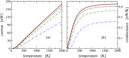
Figure 2: (Color online) Plots of (a) the steady-state current and (b) the conductance as functions of the average temperature between the two leads and with a temperature bias of $\alpha=0.1$. The values of the on-site spring constant are $k_{0}=0$ (black line), $k_{0}=0.01~{}{\rm eV/(\AA^{2}u)}$ (red dash line), $k_{0}=0.1~{}{\rm eV/(\AA^{2}u)}$ (green dash-dot line), and $k_{0}=1~{}{\rm eV/(\AA^{2}u)}$ (blue dash-double dot line). The interparticle spring constant is $k=1~{}{\rm eV/(\AA^{2}u)}$.

We first determine the steady-state heat current and conductance of an infinite linear chain using the Landauer formula with unit transmission for frequencies within the phonon band wang07 . The value of the nearest-neighbor spring constant we use is $k=1~{}{\rm eV/\AA^{2}u}$. We examine the steady-state current for on-site pinning potentials $k_{0}=0,0.01,0.1$, and $1~{}{\rm eV/\AA^{2}u}$. Shown in Fig. 2 are the plots of the steady-state thermal current and conductance as a function of the temperature. We use these results for comparison to the quasi-steady-state values arising in finite leads.

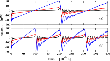
Figure 3: (Color online) Plots of the current as a function of time when the left and right chains are finite with lengths ${\rm(a)}~{}N_{\rm L}=N_{\rm R}=100$ and ${\rm(b)}~{}N_{\rm L}=N_{\rm R}=50$. The average temperatures between the leads are $T=10~{}{\rm K}$ (black line), $T=100~{}{\rm K}$ [red (gray) line], and $T=300~{}{\rm K}$ [blue (dark gray) line]. The temperature bias between the leads is $\alpha=0.1$. There is no on-site potential, i.e., $k_{0}=0$.

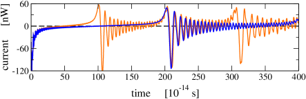
Figure 4: (Color online) A close up view of the current when the average temperature of the leads is $T=10~{}{\rm K}$. The darker (blue) line is when $N_{\rm L}=N_{\rm R}=100$ while the lighter (orange) line is when $N_{\rm L}=N_{\rm R}=50$. The dashed line is the value of the steady-state current calculated using the Landauer formula.

The dynamical energy currents are determined for various lengths and initial temperatures of the finite leads and the strengths of the on-site spring potential. Shown in Fig. 3 are plots of the current flowing out of the left lead when there is no on-site spring potential. The length of the leads are $N_{\rm L}=N_{\rm R}=100$ in Fig. 3(a) and $N_{\rm L}=N_{\rm R}=50$ in Fig. 3(b). The left lead initially has temperature $T_{\rm L}=(1+\alpha)T$, where $\alpha=0.1$, while the right lead has initial temperature $T_{\rm R}=(1-\alpha)T$. The plots in Fig. 3 correspond to $T=10~{}{\rm K}$, $100~{}{\rm K}$, and $300~{}{\rm K}$. The leads are attached at time $t=0$. Just after the switch-on, the current initially shoots down towards negative values. Since we are calculating the current flowing out of the left lead, a negative current value implies that energy is flowing into the left lead. For the right lead, we also find the same initial negative current values, i.e., energy is also flowing into the right lead. This result is the same as that found in systems with semi-infinite leads cuansing10 . The reason is because an external input energy is required to make the interleads coupling between the two previously unattached leads. After the leads are connected, the extra energy that is applied to make the connection then flows into the leads, thus initially producing negative current values just after the switch-on. This phenomenon also occurs for the leads-center system and is explained by a small $t$ expansion bijay12 .

On longer time scales, the current rises almost linearly and then suddenly drops. The overall behavior is roughly periodic with a period proportional to the full length of the chain. A ringing current can also be observed in Fig. 3. This ringing current also appears in systems containing infinite leads cuansing10 . Such a behavior has also been observed previously in NEGF calculations in electronic transport electronic . In Fig. 3, notice that the current does not stabilize to a quasi-steady-state value, even when the leads have the low average temperature $T=10~{}{\rm K}$, as shown in Fig. 4.

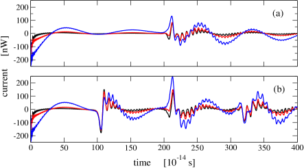
Figure 5: (Color online) Plots of the current as a function of time when the on-site spring constant is $k_{0}=0.001~{}{\rm eV/\AA^{2}u}$. The left and right chains have lengths ${\rm(a)}~{}N_{\rm L}=N_{\rm R}=100$ and ${\rm(b)}~{}N_{\rm L}=N_{\rm R}=50$. The average temperatures between the chains are $T=10~{}{\rm K}$ (black line), $T=100~{}{\rm K}$ [red (gray) line], and $T=300~{}{\rm K}$ [blue (dark gray) line]. The temperature offset is $\alpha=10\%$.

We next examine what happens to the current in the presence of a small on-site quadratic potential with on-site spring constant $k_{0}=0.001~{}{\rm eV/\AA^{2}u}$. Shown in Fig. 5 are plots of the current as it evolves in time. Compared to the current shown in Fig. 3, although there is still the initial overshoot to a negative value, the current appears to approach a quasi-steady-state value. However, the value of the on-site potential is still not enough to suppress the large current oscillations, especially when the temperature is high.

Figure 6: (Color online) Plots of the current when the on-site spring constant is $k_{0}=0.1~{}{\rm eV/\AA^{2}u}$. The left and right chains have lengths ${\rm(a)}~{}N_{\rm L}=N_{\rm R}=100$ and ${\rm(b)}~{}N_{\rm L}=N_{\rm R}=50$. The average temperatures between the chains are $T=100~{}{\rm K}$ [green (lowest gray) line], $T=300~{}{\rm K}$ [red (middle gray) line], and $T=500~{}{\rm K}$ [blue (upper gray) line]. The temperature offset is $\alpha=10\%$. The dash lines are the values of the steady-state current, corresponding to $T=100~{}{\rm K}$, $300~{}{\rm K}$, and $500~{}{\rm K}$, calculated independently from the Landauer formula.

Based on our results for the small on-site $k_{0}$, we expect the current to show a more prominent approach to a quasi-steady-state value when we increase the value of the on-site $k_{0}$ further. Shown in Fig. 6 are plots of the current when $k_{0}=0.1~{}{\rm eV/\AA^{2}u}$, i.e., at $10\%$ of the value of $k$. Also shown in the figure are dashed lines representing the steady-state current calculated using the Landauer formula. We now see that the current approaches a quasi-steady-state value and that this quasi-steady-state lasts longer for longer leads. Note, however, that the quasi-steady-state lasts for more than $2t_{m}$ ($t_{m}$ is defined to be the time when sound waves travel the left or right chain). After time $2t_{m}$, the waves or disturbances that have been reflected back at the hard walls at the edges of the leads have returned back to the interleads coupling and interfere with the other waves there. This results in the current beginning to oscillate wildly.

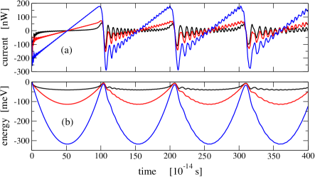
Figure 7: (Color online) Plots of (a) the current and (b) the energy as functions of time when $k_{0}=0$. The left and right chains have the same temperature, i.e., $\alpha=0$, with temperatures $T=10~{}{\rm K}$ (black line), $T=100~{}{\rm K}$ [red (gray) line], and $T=300~{}{\rm K}$ [blue (dark gray) line]. The chains have length $N_{\rm L}=N_{\rm R}=50$.

We next set the leads to have the same temperature and, therefore, according to the Landauer formula, we should not expect to have current flowing in the long-time steady-state limit. We do want to know if we get a nonzero transient current and, if so, how would it behave even when there is no temperature bias. Shown in Fig. 7 are plots of the current flowing out of the left lead when the leads have the same temperature and there is no on-site potential. Also shown are plots of the total energy that has flowed out of the left lead. The total energy at time $t$ is calculated by taking the area under the curve for the current up to time $t$. Since the leads are indistinguishable, the current plots for the left and right leads are exactly the same.

Energy is added to the system when the leads are initially attached. This energy flows into both the left and the right leads. So even when there is no temperature bias, because of the externally added energy, a thermal current appears in the system. However, because there is no on-site pinning potential, the current does not settle into a quasi-steady-state value. The phonons are elastically bouncing back and forth between the fixed walls at the edges of the two leads.

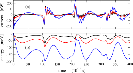
Figure 8: (Color online) Plots of (a) the current and (b) the energy as functions of time when the on-site spring constant is $k_{0}=0.001~{}{\rm eV/\AA^{2}u}$. The left and right chains have the same temperature of values $T=10~{}{\rm K}$ (black line), $T=100~{}{\rm K}$ [red (gray) line], and $T=300~{}{\rm K}$ [blue (dark gray) line]. The chains have length $N_{\rm L}=N_{\rm R}=50$.

Shown in Fig. 8 are plots of the current and total energy when a small on-site potential with $k_{0}=0.001~{}{\rm eV/\AA^{2}u}$ is present in the system. The presence of the on-site pinning potential suppresses the current to a quasi-steady-state value. The total energy shown in Fig. 8(b) also displays a tendency to settle down to a quasi-steady-state value.

Figure 9: (Color online) Plot of the energy as a function of time. The inset shows the plot of the current as a function of time. The left and right chains have the same temperature $T=300~{}{\rm K}$ and the on-site spring constant is $k_{0}=0.1~{}{\rm eV/\AA^{2}u}$. The chains have length $N_{\rm L}=N_{\rm R}=50$.

Shown in Fig. 9 are plots of the current and total energy when the on-site potential has spring constant $k_{0}=0.1~{}{\rm eV/(\AA^{2}u)}$. The value is large enough for the current to settle into a quasi-steady-state value. However, since the leads are finite, the system only has limited time before the reflected phonons begin to arrive and interfere with the other phonons moving through the interleads coupling.

We can also calculate the current at sites away from the midpoint of the composite system where the sudden attachments occurred using Eq. (15). For a composite lead containing $N_{\rm L}=100$ and $N_{\rm R}=100$ sites, we determine the current at sites $n_{1}=N_{\rm L}+50$ and $n_{2}=N_{\rm L}+75$. Shown in Figs. 10 and 11 are plots of the current at those locations. In Fig. 10 the spring constant is $1~{}{\rm eV/(\AA^{2}u)}$ and there is no on-site potential. Because $n_{1}$ and $n_{2}$ are away from the midpoint, the current is going to take some time, depending on how fast phonons travel in the chain, to reach them. Defining a time unit $[{\rm t}]\equiv 10^{-14}\,{\rm s}$, it takes $50\,[{\rm t}]$ for the current to reach $n_{1}$ and $75\,[{\rm t}]$ to reach $n_{2}$, therefore implying a speed of $1$ site per $[{\rm t}]$.

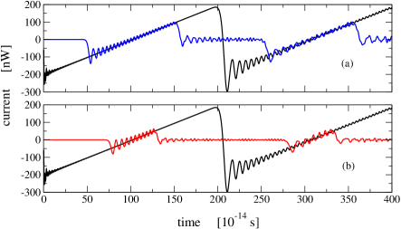
Figure 10: (Color online) Plots of the current at various locations on the right lead. The length of the left and right leads are $N_{\rm L}=N_{\rm R}=100$. The darker (black) lines in both panels (a) and (b) are the current at $N_{\rm L}$. The current at $n_{1}=N_{\rm L}+50$ [blue (dark gray) line in panel (a)] and $n_{2}=N_{\rm L}+75$ [red (gray) line in panel (b)] are also shown. The on-site spring constant is $k_{0}=0$ and the temperature $T=300~{}{\rm K}$.

In Fig. 11 a quadratic on-site potential with spring constant $k_{0}=0.1~{}{\rm eV/(\AA^{2}u)}$ is added to the system. The two leads have the same temperature $T=300~{}{\rm K}$. For the midpoint where the sudden connection at $t=0$ occurs, upon connection the current immediately drops and then oscillates and decays until it reaches a quasi-steady-state value which, for this case, is zero. Away from the midpoint, the current takes some time to reach the site and so initially we see a flat line at zero. Since $k_{0}$ is not zero, the speed of the current is not exactly $1$ site per $[{\rm t}]$ as we found in Fig. 10.

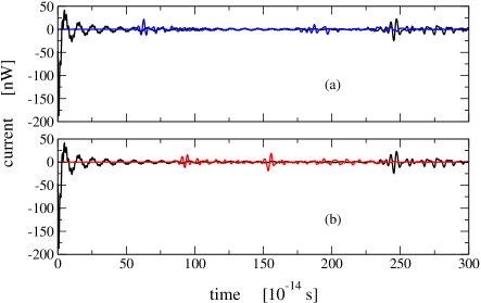
Figure 11: (Color online) Plots of the current at different locations on the right lead when $N_{\rm L}=N_{\rm R}=100$, $T=300~{}{\rm K}$, and on-site spring constant $k_{0}=0.1~{}{\rm eV/\AA^{2}u}$. The darker (black) lines in both panels (a) and (b) are the current at $N_{\rm L}$. The current at $n_{1}$ [blue (dark gray) line in panel (a)] and $n_{2}$ [red (gray) line in panel (b)] are also shown.

V Summary and conclusion

We examine the energy current in a quantum system consisting of two finite chains that are abruptly attached at time $t=0$. We calculate the current using an eigenmode approach that makes use of a similarity transformation extending the normal modes of a single harmonic oscillator into a many-particle, but finite, chain of harmonic oscillators. In addition, we use a nonequilibrium Green’s function approach to verify some of the results from our normal mode calculations. We find that the presence of a quadratic on-site pinning potential is crucial in establishing a quasi-steady-state current. In a finite system where there is no such on-site potential, the current does not settle to a quasi-steady-state value, even when the two original chains have the same temperature at a value as low as $10~{}{\rm K}$. The phonons would simply bounce back and forth elastically between the two fixed walls at the edges of the chains. In the presence of the on-site pinning potential, we find a tendency for the current to establish a quasi-steady state (also, see the Appendix). This crucial role of the on-site pinning potential in establishing a steady-state current should also be present even when the leads are semi-infinite. Computationally, the presence of the quadratic on-site pinning potential renders well-behaved Green’s functions. The form of the time evolution of the current depends on the interplay between the strength of the potentials, the chain length, and the initial chain temperatures. A quasi-steady-state current is established earlier when the on-site pinning potential is stronger. Furthermore, when the quasi-steady-state current is established, its value turns out to be the same as the steady-state value calculated using the Landauer formula. Although in the standard modeling of bosonic heat baths infinite systems are usually employed, we show here that integrable finite systems also behave like an infinite system but only within short time scales proportional to the system size $N$ and provided that a small on-site pinning potential is present. At time scales longer than $N$, we have recurrent and quasi-periodic behavior. It is interesting to investigate what happens if the chains are nonlinear; however, the eigenmode expansion technique discussed in this paper is unable to handle nonlinear systems.

Appendix A Recovering the Landauer formula

In this appendix, we simplify the formula for the current based on Eqs. (12) to (14) and derive the Landauer formula in the large-size limit. We first introduce a new notation and then group the terms into two parts. The first part involves terms that are proportional to the difference between the Bose distributions of the left and right leads. The rest of the terms constitutes the other part and are interpreted to be the transient contribution to the current. We assume that each chain has length $N$ and, therefore, that the total size of the composite chain is $2N$. Define

$$\begin{split}\left<k|\right.{\tilde{k}}\left.\right>^{\rm L}&\equiv\sum_{n_{1}=1}^{N}\left<k|n_{1}\right>\!\left<n_{1}\right|{\tilde{k}}\left.\right>,\\ \left<k|\right.{\tilde{k}}\left.\right>^{\rm R}&\equiv\sum_{n_{1}=N+1}^{2N}\left<k|n_{1}\right>\!\left<n_{1}-N\right|{\tilde{k}}\left.\right>,\end{split}$$ (18)

where $\left<n\right.|{\tilde{k}}\left.\right>=\left<\right.{\tilde{k}}|\left.n\right>\equiv\sqrt{\frac{2}{N+1}}\,\sin({\tilde{k}}n)$, ${\tilde{k}}=\frac{\pi{\tilde{j}}}{N+1}$, $\left<k|n\right>=\left<n|k\right>\equiv\sqrt{\frac{2}{2N+1}}\sin(kn)$, and $k=\frac{\pi j}{2N+1}$. Notice that $\left<k\right.|{\tilde{k}}\left.\right>^{\rm R}=\left<k|\right.{\tilde{k}}\left.\right>^{\rm L}\left(-1\right)^{j+{\tilde{j}}}$ and $\left<\right.{\tilde{k}}|\left.k_{2}\right>^{\rm L}\!\left<k_{2}\right.|{N+1}\left.\right>=\left<\right.{\tilde{k}}|\left.k_{2}\right>^{\rm L}\!\left<k_{2}\right.|N\left.\right>\left(-1\right)^{j_{2}+1}$. The expression for the current $I^{\rm L}(t)$ can be separated into two parts, $I^{\rm L}_{{\rm trans}}(t)$ and $I^{\rm L}_{{\rm stdy}}(t)$, where the transient contribution is

$$\begin{split}I^{\rm L}_{{\rm trans}}(t)&=\hbar\omega_{0}^{2}\,\sum_{\tilde{k}}\left(f_{\tilde{k}}^{\rm L}+f_{\tilde{k}}^{\rm R}+1\right)\\ &\times\sum_{k_{1}\,{\rm odd}}\left(\frac{\omega_{k_{1}}}{\omega_{\tilde{k}}}-\frac{\omega_{\tilde{k}}}{\omega_{k_{1}}}\right)\sin\left(\omega_{k1}t\right)\,\left<N|k_{1}\right>\!\left<k_{1}\right|{\tilde{k}}\left.\right>^{\rm L}\\ &\times\sum_{k_{2}\,{\rm odd}}\cos\left(\omega_{k_{2}}t\right)\,\left<\right.{\tilde{k}}|\left.k_{2}\right>^{\rm L}\!\left<k_{2}|N\right>\\ -\,\hbar\omega_{0}^{2}&\,\sum_{\tilde{k}}\left(f_{\tilde{k}}^{\rm L}+f_{\tilde{k}}^{\rm R}+1\right)\\ &\times\sum_{k_{1}\,{\rm even}}\left(\frac{\omega_{k_{1}}}{\omega_{\tilde{k}}}-\frac{\omega_{\tilde{k}}}{\omega_{k_{1}}}\right)\sin\left(\omega_{k_{1}}t\right)\,\left<N\right|k_{1}\left.\right>\!\left<k_{1}\right|{\tilde{k}}\left.\right>^{\rm L}\\ &\times\sum_{k_{2}\,{\rm even}}\cos\left(\omega_{k_{2}}t\right)\left<\right.{\tilde{k}}|k_{2}\left.\right>^{\rm L}\!\left<k_{2}|N\right>.\end{split}$$ (19)

and the steady-state contribution is

$$\begin{split}I^{\rm L}_{{\rm stdy}}(t)&=\hbar\omega_{0}^{2}\,\sum_{\tilde{k}}\left(f_{\tilde{k}}^{L}-f_{\tilde{k}}^{R}\right)\\ &\times\sum_{k_{1}\,{\rm even}}\left(\frac{\omega_{k_{1}}}{\omega_{\tilde{k}}}+\frac{\omega_{\tilde{k}}}{\omega_{k_{1}}}\right)\sin\left(\omega_{k_{1}}t\right)\,\left<N|k_{1}\right>\!\left<k_{1}\right|{\tilde{k}}\left.\right>^{\rm L}\\ &\times\sum_{k_{2}\,{\rm odd}}\cos\left(\omega_{k_{2}}t\right)\left<\right.{\tilde{k}}|k_{2}\left.\right>^{\rm L}\!\left<k_{2}|N\right>\\ -\,\hbar\omega_{0}^{2}&\,\sum_{\tilde{k}}\left(f_{\tilde{k}}^{L}-f_{\tilde{k}}^{\rm R}\right)\\ &\times\sum_{k_{1}\,{\rm even}}\cos\left(\omega_{k_{1}}t\right)\,\left<N|k_{1}\right>\!\left<k_{1}\right|{\tilde{k}}\left.\right>^{\rm L}\\ &\times\sum_{k_{2}\,{\rm odd}}\left(\frac{\omega_{\tilde{k}}}{\omega_{k_{2}}}+\frac{\omega_{k_{2}}}{\omega_{\tilde{k}}}\right)\sin\left(\omega_{k_{2}}t\right)\,\left<\right.{\tilde{k}}|\left.k_{2}\right>^{\rm L}\!\left<k_{2}|N\right>.\end{split}$$ (20)

In the above, the summation for $\tilde{k}$ extends over all $\frac{\pi\tilde{j}}{N+1}$ for ${\tilde{j}}=1,...,N$, the summation involving “$k_{1}$ even” is on $k_{1}\in\left\{\frac{\pi j_{1}}{2N+1}\right\}_{j_{1}=1}^{2N}$, $j_{1}$ is even, and the summation involving “$k_{2}$ odd” is on $k_{2}\in\left\{\frac{\pi j_{2}}{2N+1}\right\}_{j_{2}=1}^{2N}$, $j_{2}$ is odd, and so on. The dispersion relation satisfied is $\omega_{q}=\sqrt{2k\left(1-\cos q\right)+k_{0}}$ where $\omega_{0}^{2}=k$, $\omega_{1}^{2}=k_{0}$, $f_{\tilde{k}}^{\alpha}=1/(e^{\beta_{\alpha}\hbar\omega_{\tilde{k}}}-1)$, and $\alpha={\rm L,R}$. The sum in Eq. (18) can be carried out analytically, resulting in

$$\begin{split}\left<N|k_{1}\right>\!\left<k_{1}\right|{\tilde{k}}\left.\right>^{\rm L}&=\frac{-1}{(2N+1)\sqrt{2(N+1)}}\\ &\times\sin({\tilde{k}}N)\,\frac{\cos k_{1}-\left(-1\right)^{j_{1}}}{\cos{\tilde{k}}-\cos k_{1}}.\end{split}$$ (21)

A similar expression can be derived for $\left<\right.{\tilde{k}}|\left.k_{2}\right>^{\rm L}\!\left<k_{2}|N\right>$. Using Eqs. (19) to (21), the current can now be calculated in computer time proportional to ${\mathit{O}}(N^{2})$. This is in contrast to NEGF calculations which go as ${\mathit{O}}(N^{3})$ in computational complexity.

All of the expressions derived at this point are exact. We now make an approximation in order to extend our calculations for the steady-state contribution to large $N$ and eventually arrive at the Landauer formula. Notice that in Eq. (21) and the corresponding expression for $k_{2}$ that the terms involving $k_{1}\approx\tilde{k}\approx k_{2}$ would dominate the summation, especially when $N$ approaches infinity. Consequently,

$$\begin{split}I^{\rm L}_{{\rm stdy}}(t)\approx&\,\hbar\omega_{0}^{2}\,\frac{1}{N+1}\sum_{\tilde{k}}\left(f_{\tilde{k}}^{\rm L}-f_{\tilde{k}}^{\rm R}\right)\sin^{4}\tilde{k}\\ &\times\left\{\frac{1}{2N+1}\,\frac{1}{2}\sum_{k_{2}}\frac{\sin\left(\omega_{\tilde{k}}-\omega_{k_{2}}\right)t}{\cos\tilde{k}-\cos k_{2}}\right\}\\ &\times\left\{\frac{1}{2N+1}\left\{\sum_{k_{1}=e}\frac{-1}{\cos\tilde{k}-\cos k_{1}}\right.\right.\\ &\;\;\;+\left.\left.\sum_{k_{1}\,{\rm odd}}\frac{1}{\cos\tilde{k}-\cos k_{1}}\right\}\right\}.\end{split}$$ (22)

Let $N\rightarrow\infty$ and then followed by $t\rightarrow\infty$, we get

$$\frac{1}{2N+1}\,\frac{1}{2}\sum_{k_{2}}\frac{\sin\left(\omega_{\tilde{k}}-\omega_{k_{2}}\right)t}{\cos\tilde{k}-\cos k_{2}}\approx-\frac{1}{2\sin\tilde{k}}.$$ (23)

Furthermore, we have

$$\begin{split}\lim_{N\rightarrow\infty}\frac{1}{2N+1}&\left\{\sum_{k_{1}\,{\rm even}}\frac{-1}{\cos{\tilde{k}}-\cos k_{1}}\right.\\ &+\left.\sum_{k_{1}\,{\rm odd}}\frac{1}{\cos\tilde{k}-\cos k_{1}}\right\}=-\frac{1}{\sin^{2}{\tilde{k}}}\end{split}$$ (24)

for some $\tilde{k}\in\left\{\frac{\pi\tilde{j}}{N+1}\right\}_{\tilde{j}=1}^{N}$. We then recover the Landauer formula

$$\begin{split}I^{\rm L}_{{\rm stdy}}&=\frac{1}{2}\,\hbar\omega_{0}^{2}\,\frac{1}{N+1}\sum_{\tilde{k}}\left(f_{\tilde{k}}^{\rm L}-f_{\tilde{k}}^{\rm R}\right)\sin\tilde{k}\\ &=\frac{1}{2\pi}\int_{\omega_{1}}^{\sqrt{4\omega_{0}^{2}+\omega_{1}^{2}}}d\omega\,\hbar\omega\left(f^{\rm L}(\omega)-f^{\rm R}(\omega)\right).\end{split}$$ (25)

Note in the above that the discrete summation over wave vector $\tilde{k}$ is converted into a continuous integration over the angular frequency $\omega$. Furthermore, we want to emphasize that although the on-site constant $k_{0}$ appears in the expressions for both $I_{\rm stdy}$ and $I_{\rm trans}$, its presence in the steady-state contribution $I_{\rm stdy}$ does not prevent the contribution to approach a steady-state value in the long-time limit. In contrast, the value of $k_{0}$ is crucial for the transient contribution $I_{\rm trans}$ to decay away. A zero $k_{0}$ would result in $I_{\rm trans}$ having a strong time-dependent zigzag-like behavior that would dominate the total energy current at all times. There would be no steady current flow even when $N\rightarrow\infty$. However, even a small on-site potential, say $k_{0}/k=0.1$, would result in the transient contribution to decay away in the long-time limit and leave only the contribution from the steady-state term.

References

• (1) See, for a review, J.-S. Wang, J. Wang, and J.T. Lü, Eur. Phys. J. B 62, 381 (2008).
• (2) E.C. Cuansing and J.-S. Wang, Phys. Rev. B 81, 052302 (2010); E.C. Cuansing and J.-S. Wang, ibid. 83, 019902(E) (2011); E.C. Cuansing and J.-S. Wang, Phys. Rev. E 82, 021116 (2010).
• (3) M. Campisi, P. Talkner, and P. Hänggi, Phys. Rev. E 80, 031145 (2009).
• (4) D. Roy and A. Dhar, Phys. Rev. E 78, 051112 (2008); A. Chaudhuri, A. Kundu, D. Roy, A. Dhar, J.L. Lebowitz, and H. Spohn, Phys. Rev. B 81, 064301 (2010).
• (5) H.L. Frisch, Phys. Rev. 104, 1 (1956); P.Chr. Hemmer, L.C. Maximon, and H. Wergeland, ibid. 111, 689 (1958); M. Kac, ibid. 115, 1 (1959); J.A. McLennan, Phys. Fluids 2, 92 (1959).
• (6) R. Zwanzig, Nonequilibrium Statistical Mechanics (Oxford University Press, New York, 2001).
• (7) P. Bocchieri and A. Loinger, Phys. Rev. 114, 948 (1959); K. Battacharyya and D. Mukherjee, J. Chem. Phys. 84, 3212 (1986).
• (8) T. Hogg and B.A. Huberman, Phys. Rev. Lett. 48, 711 (1982); T. Hogg and B.A. Huberman, Phys. Rev. A 28, 22 (1983).
• (9) N. Bushong, N. Sai, and M. Di Ventra, Nano Lett. 5, 2569 (2005).
• (10) J.-W. Jiang, J.-S. Wang, and B. Li, Phys. Rev. B 80, 205429 (2009).
• (11) J.-S. Wang, N. Zeng, J. Wang, and C.K. Gan, Phys. Rev. E 75, 061128 (2007).
• (12) B.K. Agarwalla, B. Li, and J.-S. Wang, Phys. Rev. E 85, 051142 (2012).
• (13) A.-P. Jauho, N.S. Wingreen, and Y. Meir, Phys. Rev. B 50, 5528 (1994); J. Maciejko, J. Wang, and H. Guo, ibid. 74, 085324 (2006); Y. Zhu, J. Maciejko, T. Ji, H. Guo, and J. Wang, ibid. 71, 075317 (2005); E. Perfetto, G. Stefanucci, and M. Cini, ibid. 82, 035446 (2010).