Multiple-Source Multiple-Sink Maximum Flow in Directed Planar Graphs in Near-Linear Time

We give an $O(n\log^{3}n)$ algorithm that, given an $n$-node directed planar graph with arc capacities, a set of source nodes, and a set of sink nodes, finds a maximum flow from the sources to the sinks. Previously, the fastest algorithms known for this problem were those for general graphs.

1 Introduction

The maximum flow problem with multiple sources and sinks in a directed graph with arc-capacities is, informally, to find a way to route a single commodity from a given set of sources to a given set of sinks such that the total amount of the commodity that is delivered to the sinks is maximum subject to each arc carrying no more than its capacity. In this paper we study this problem in planar graphs.

The study of maximum flow in planar graphs has a long history. In 1956, Ford and Fulkerson introduced the max $st$-flow problem, gave a generic augmenting-path algorithm, and also gave a particular augmenting-path algorithm for the case of a planar graph where $s$ and $t$ are on the same face Researchers have since published many algorithmic results proving running-time bounds on max $st$-flow for (a) planar graphs where $s$ and $t$ are on the same face, (b) undirected planar graphs where $s$ and $t$ are arbitrary, and (c) directed planar graphs where $s$ and $t$ are arbitrary. The best bounds known are (a) $O(n)$ [14], (b) $O(n\log\log n)$ [17], and (c) $O(n\log n)$ [2], where $n$ is the number of nodes in the graph.

Maximum flow in planar graphs with multiple sources and sinks was studied by Miller and Naor [29]. When it is known how much of the commodity is produced/consumed at each source and each sink, finding a consistent routing of flow that respects arc capacities can be reduced to negative-length shortest paths, which we now know can be solved in planar graphs in $O(n\log^{2}n/\log\log n)$ time [30]. Otherwise, Miller and Naor gave an $O(n\log^{3/2}n)$ algorithm for the case where all the sinks and the sources are on the boundary of a single face, and generalized it to an $O(k^{2}n^{3/2}\log^{2}n)$-time algorithm for the case where the sources and the sinks reside on the boundaries of $k$ different faces.

However, the problem of maximum flow with multiple sources and sinks in planar graphs without any additional restrictions remained open. In general (i.e., non-planar) graphs, multiple sources and sinks can be reduced to the single-source single-sink case by introducing an artificial source and sink and connecting them to all the sources and sinks, respectively—but this reduction does not preserve planarity. For more than twenty years since the problem was explicitly stated and considered [29], the fastest known algorithm for computing multiple-source multiple-sink max-flow in a planar graph has been to use this reduction in conjunction with a general maximum-flow algorithm such as that of Sleator and Tarjan [32] which leads to a running time of $O(n^{2}\log n)$. For integer capacities less than $U$, one could instead use the algorithm of Goldberg and Rao [10], which leads to a running time of $O(n^{1.5}\log n\log U)$. No planarity-exploiting algorithm was known for the problem.

Our Result

The main result of this paper is an algorithm for the problem that is optimal up to a small poly-logarithmic factor.

Theorem 1.1.

There exists an algorithm that solves the maximum flow problem with multiple sources and sinks in an $n$-node directed planar graph in $O(n\log^{3}n)$ time.

Application to computer vision problems

Multiple-source multiple-sink min-cut arises in addressing a family of problems associated with the terms metric labeling (Kleinberg and Tardos, [26]), Markov Random Fields [9], and Potts Model (see also [4, 15]). In low-level vision problems such as image restoration, segmentation, stereo, and motion, the goal is to assign labels from a set to pixels so as to minimize a penalty function. The penalty function is a sum of two parts. One part, the data component, has a term for each pixel; the cost depends on the discrepancy between the observed data for the pixel and the label chosen for it. The other part, the smoothing component, penalizes neighboring pixels that are assigned different labels.

For the binary case (when the set of available labels has size two), finding the optimal solution is reducible to multiple-source multiple-sink min-cut. [12]. For the case of more than two labels, there is a powerful and effective heuristic [4] using very-large-neighborhood [1] local search; the inner loop consists of solving the two-label case. The running time for solving the two-label case is therefore quite important. For this reason, researchers in computer vision have proposed new algorithms for max flow and done experimental studies comparing the run-times of different max-flow algorithms on the instances arising in this context [3, 27]. All of this is evidence for the importance of the problem.

For the (common) case where the underlying graph of pixels is the two-dimensional grid graph, our result yields a theoretical speed-up for this important computer-vision subroutine.

Hochbaum [15] describes a special case of the penalty function in which the data component is convex and the smoothing component is linear; in this case, she shows that an optimal solution can be found in time $O(T(m,n)+n\log U)$ where $U$ is the maximum label, and $T(m,n)$ is the time for finding a minimum cut. She mentions specifically image segmentation, for which the graph is planar. For this case, by using our algorithm, the optimal solution can be found in nearly linear time

Application to maximum bipartite matching

Consider the problem of maximum matching in a bipartite planar graph. It is well-known how to reduce this problem to multiple-source, multiple-sink maximum flow. Our result is the first planarity-exploiting algorithm for this problem (and the first near-linear one).

Techniques

To obtain our result, we employ a wide range of sophisticated algorithmic techniques for planar graphs, some of which we adapted to our needs while others are used unchanged. Our algorithm uses pseudoflows [11, 16] and a divide-and-conquer scheme influenced by that of [19] and that of [29]. We adapt a method for using shortest paths to solve max $st$-flow when $s$ and $t$ are adjacent [13], and a data structure for implementing Dijkstra in a dense distance graph derived from a planar graph [8]. Among the other techniques we employ are: using cycle separators [28] recursively while keeping the boundary nodes on a constant number of faces [25, 33, 8], an algorithm for single-source single-sink max flow [2, 7], an algorithm for computing multiple-source shortest paths [23, 5], a method for cancelling cycles of flow in a planar graph [20], an algorithm for finding shortest paths in planar directed graphs with negative lengths [24, 30], and a data structure for range queries in a Monge matrix [21].

1.1 Preliminaries

We assume the reader is familiar with the basic definitions of planar embedded graphs and their duals (cf.  [2]). Let $G=(V,E)$ be a planar embedded graph with node-set $V$ and arc-set $E$. We use the term arc to emphasize that edges are directed. The term edge is used when the direction of an arc is not important. For each arc $a$ in the arc-set $E$, we define two oppositely directed darts, one in the same orientation as $a$ (which we sometimes identify with $a$) and one in the opposite orientation [2]. We define $\mbox{rev}(\cdot)$ to be the function that takes each dart to the corresponding dart in the opposite direction. It is notationally convenient to equate the edges, arcs and darts of $G$ with the edges, arcs and darts of the dual $G^{*}$.

Let $S\subset V$ be a set of nodes called sources, and let $T\subseteq V-S$ be a set of nodes called sinks.

A flow assignment $\bm{f}(\cdot)$ is a real-valued function on darts satisfying antisymmetry:

$$\bm{f}(\mbox{rev}(d))=-\bm{f}(d)$$

A capacity assignment $\bm{c}(\cdot)$ is a real-valued function on darts.

A flow assignment $\bm{f}(\cdot)$ respects the capacity of dart $d$ if $\bm{f}(d)\leq\bm{c}(d)$. $\bm{f}(\cdot)$ is called a pseudoflow if it respects the capacities of all darts.

For a given flow assignment $\bm{f}(\cdot)$, the net inflow (or just inflow) node $v$ is $\textrm{inflow}_{\bm{f}}(v)=\sum_{\textrm{dart }d:\text{head}(d)=v}\bm{f}(d)$. The outflow of $v$ is $\textrm{outflow}_{\bm{f}}(v)=-\textrm{inflow}_{\bm{f}}(v)$. A flow assignment $\bm{f}(\cdot)$ is said to obey conservation at node $v$ if $\textrm{inflow}_{\bm{f}}(v)=0$. A feasible flow is a pseudoflow that obeys conservation at every node other than the sources and sinks. A feasible circulation is a pseudoflow that obeys conservation at all nodes. The value of a feasible flow $\bm{f}(\cdot)$ is the sum of inflow at the sinks, $\sum_{t\in T}\textrm{inflow}_{\bm{f}}(t)$ or, equivalently, the sum of outflow at the sources. The maximum flow problem is that of finding a feasible flow with maximum value.

For two flow assignments $\bm{f},\bm{f}^{\prime}$, the addition $\bm{f}+\bm{f}^{\prime}$ is the flow that assigns $\bm{f}(d)+\bm{f}^{\prime}(d)$ to every dart $d$.

A residual path in $G$ is a path whose darts all have strictly positive capacities. For two sets of nodes $A,B$, $A\stackrel{{\scriptstyle G}}{{\rightarrow}}B$ is used to denote the existence of some residual $a$-to-$b$ path in $G$ for some nodes $a\in A$ and $b\in B$. Conversely, $A\stackrel{{\scriptstyle G}}{{\nrightarrow}}B$ is used to denote that no such path exists. We will omit the graph $G$ when it is clear from the context.

The residual graph of $G$ with respect to a flow assignment $\bm{f}(\cdot)$ is the graph $G_{\bm{f}}$ with the same arc-set, node-set, sources and sinks, and with capacity assignment $\bm{c}_{\bm{f}}(\cdot)$ such that for every dart $d$, $\bm{c}_{\bm{f}}(d)=\bm{c}(d)-{\bm{f}}(d)$. It is well known that a feasible flow $\bm{f}$ in $G$ is maximum if and only if $S\stackrel{{\scriptstyle G_{{\bm{f}}}}}{{\nrightarrow}}T$.

Let $\bm{f}$ be a pseudoflow in a planar graph $G$. Let $V^{+}$ denote the set of nodes $\{v\in V-(S\cup T):\textrm{inflow}_{\bm{f}}(v)>0\}$. Similarly, let $V^{-}$ denote the set of nodes $\{v\in V-(S\cup T):\textrm{inflow}_{\bm{f}}(v)<0\}$. Suppose $S\cup V^{+}\stackrel{{\scriptstyle G_{\bm{f}}}}{{\nrightarrow}}T\cup V^{-}$. For a graph with $n$ nodes and $m$ edges, there exists an $O(m\log n)$-time algorithm that converts the pseudoflow $\bm{f}$ into a maximum feasible flow $\bm{f}^{\prime}$ [19, 32]. In planar graphs, this can be done in linear time by first canceling flow cycles using the technique of Kaplan and Nussbaum [20], and then by sending back flow from $V^{+}$ and into $V^{-}$ in topological sort order. See Appendix C for details.

1.2 Overview of the algorithm

Consider the following recursive approach for finding a maximum multiple-source multiple-sink flow: split the input graph $G$ in two using a simple cycle separator $C$ [28] and recursively solve the max flow problem in the two subgraphs. When the two recursive calls have been executed, in each of the two subgraphs there is no residual path from any source to any sink. If we further make sure that in each of the two subgraphs there is no residual path from any source to $C$ and from $C$ to any sink, then, since $C$ is a separator, there is no residual path from any source to any sink in $G$.

We therefore solve a slightly more general problem recursively in the two subgraphs: roughly speaking, find a flow such that there is no residual path from a source to a sink or to $C$ and no residual path from $C$ to a sink (Section 2). After the two recursive calls there is no residual path from any source to any sink in $G$. However, the requirement that there is no residual path from any source to $C$ and from $C$ to any sink cannot be achieved by a feasible flow but rather by a pseudoflow in which there might be excess inflow or excess outflow on nodes of $C$. We deal with this by solving a new max flow problem where nodes of $C$ are treated as sources and sinks, limited in supply/demand by their excess inflow/outflow (Section 3).

We exploit a relation between primal circulations and dual shortest paths to maintain a succinct representation of the flow during critical phases of the algorithm, using the fact that there are only $O(\sqrt{n})$ sources and sinks, all cyclically ordered on $C$ (Section  3.2). Even though our representation does not explicitly store the flow on nearly any arc in the graph, we can augment it efficiently towards optimality while maintaining feasibility. An important tool we use is Fakcharoenphol and Rao’s efficient implementation of Dijkstra’s algorithm [8], which we adapt to our needs.

The resulting pseudoflow can then be turned into a max flow in linear time using existing techniques (Appendix C). This leads to an $O(n\log^{3}n)$ time algorithm for max flow.

2 The Algorithm

Now we describe the algorithm, referred to as MultipleSourceMultipleSinkMaxFlow, in more detail. In order to treat nodes of the cycle separator both as sources and as sinks in recursive calls, we introduce a new node set $A$. At the top recursion level, $A=\emptyset$. In general, $A$ has constant size; more precisely $|A|\leq 6$.

MultipleSourceMultipleSinkMaxFlow($G,\bm{c}$,$S$,$T$,$A$)
Input: a directed planar graph $G$ with non-negative capacities $\bm{c}$, a set $S$ of source nodes, a set $T$ of sink nodes, a set $A$ of at most six nodes
Output: a pseudoflow $\bm{f}$ obeying conservation everywhere but $S,T,A$ and s.t. $S\stackrel{{\scriptstyle G_{\bm{f}}}}{{\nrightarrow}}T$, $S\stackrel{{\scriptstyle G_{\bm{f}}}}{{\nrightarrow}}A$, $A\stackrel{{\scriptstyle G_{\bm{f}}}}{{\nrightarrow}}T$.

The algorithm finds a simple cycle separator $C$ [28] and contracts all edges of $C$ except one. This, essentially, merges all the nodes of $C$ into a single supernode $v$, and turns $C$ into a self loop. For simplicity of presentation we assume that no sources or sinks lie on $C$. The algorithm then recursively solves the problem on the subgraphs enclosed and not enclosed by that self loop (the self loop itself need not be included in any of the subgraphs), adding the supernode $v$ that represents $C$ to the set $A$. In order to keep the cardinality of $A$ at most six, the algorithm alternately applies the cycle separator theorem with weights uniformly distributed on all nodes and uniformly distributed on only the nodes of $A$. This technique is similar to that used in [25, 33, 8].

After the recursive calls, the algorithm uncontracts the edges of $C$. At this stage there are no residual paths between sources and sinks in the entire graph, but there might be excess inflow (positive or negative) at the nodes of $C$. The algorithm then calls the procedure FixConservationOnPath that pushes flow between the nodes of $C$ so that there are no residual paths between nodes of $C$ with positive inflow and nodes of $C$ with negative inflow (the path in the name of the procedure is the cycle $C$ without one edge). This procedure is discussed in Section 3; the interface is:

FixConservationOnPath$(G,P,\bm{c},\bm{f}_{0})$
Input: a directed planar graph $G$, simple path $P$, capacity function $\bm{c}$, and a pseudoflow $\bm{f}_{0}$
Output: a pseudoflow $\bm{f}$ s.t. (i) $\bm{f}-\bm{f}_{0}$ satisfies conservation everywhere but $P$, and
(ii) $\{v\in P:\textrm{inflow}(v)>0\}\stackrel{{\scriptstyle G_{\bm{f}}}}{{\nrightarrow}}\{v\in P:\textrm{inflow}(v)<0\}$.
Running Time: $O(n\log^{2}n/\log\log n+|P|^{2}\log^{2}n)$

Next, the algorithm iterates over the nodes $a_{i}$ of $A$. The algorithm calls the procedure CycleToSingleSinkLimitedMaxFlow that, roughly speaking, pushes as much excess flow as possible from $C$ to $a_{i}$. If $C_{i}^{+}$ is the set of nodes of $C$ that are reachable via residual paths from some node of $C$ with positive inflow at the beginning of iteration $i$, CycleToSingleSinkLimitedMaxFlow pushes flow among the nodes of $C_{i}^{+}$ and from the nodes of $C_{i}^{+}$ to $a_{i}$. The result is that remaining inflow at nodes of $C_{i}^{+}$ is non-negative and there are no residual paths from nodes of $C$ with positive inflow to $a_{i}$. See Section 4; the interface is:

CycleToSingleSinkLimitedMaxFlow($G,\bm{c},\bm{f}_{0},C,a_{i}$)
Input: a directed planar graph $G$ with capacities $\bm{c}$, a pseudoflow $\bm{f}_{0}$, a simple cycle $C$, a sink $a_{i}$.
Assumes: $\forall v\in C^{+},\ \textrm{inflow}_{\bm{f}_{0}}(v)\geq 0$, where $C^{+}=\{v\in C:\{x\in C:\textrm{inflow}_{\bm{f}_{0}}(x)>0\}\stackrel{{\scriptstyle G_{\bm{f}_{0}}}}{{\rightarrow}}v\}$.
Output: a pseudoflow $\bm{f}$ s.t. (i) $\bm{f}-\bm{f}_{0}$ obeys conservation everywhere but $C^{+}\cup\{t\}$, (ii) $\forall v\in C^{+},\ \textrm{inflow}_{\bm{f}}(v)\geq 0$, (iii) $\{v\in C:\textrm{inflow}_{\bm{f}}(v)>0\}\stackrel{{\scriptstyle G_{\bm{f}}}}{{\nrightarrow}}a_{i}$.
Running Time: $O(n\log^{2}n/\log\log n+|C|^{2}\log^{2}n)$.

A similar procedure SingleSourceToCycleLimitedMaxFlow is called to push flow from $a_{i}$ to $C$ to eliminate as much negative inflow as possible (using a similarly defined set $C_{i}^{-}$).

Finally, the algorithm pushes back flow from any nodes of $C$ with positive inflow to $S$ and pushes flow back from $T$ into any nodes of $C$ with negative inflow.

Algorithm 1 MultipleSourceMultipleSinkMaxFlow($G,\bm{c}$,$S$,$T$,$A$)

Input: a directed planar graph $G$ with non-negative capacities $\bm{c}$, a set $S$ of source nodes, a set $T$ of sink nodes, a set $A$ consisting of a constant number of nodes $A=\{a_{i}\}_{i=1}^{k}$.
Output: a pseudoflow $\bm{f}$ obeying conservation everywhere except $S,T,A$ and s.t. $S\stackrel{{\scriptstyle G_{\bm{f}}}}{{\nrightarrow}}T$, $S\stackrel{{\scriptstyle G_{\bm{f}}}}{{\nrightarrow}}A$, $A\stackrel{{\scriptstyle G_{\bm{f}}}}{{\nrightarrow}}T$.

1:  add zero capacity arcs to triangulate and 2-connect $G$ (required for simple cycle separators)

2:  find a balanced (w.r.t. $|G|$ and $|A|$, alternately) cycle separator $C$ in $G$ disjoint from $S$ and $T$

3:  let $P$ be a path comprising of all of $C$’s edges except one edge $e$

4:  contract all the edges of $P$, turning $e$ into a self loop incident to the only remaining node $v$ of $C$

5:  let $G_{1}$ and $G_{2}$ be the subgraph of $G$ enclosed and not enclosed by $e$, respectively

6:  $\bm{f}:=$ MultipleSourceMultipleSinkMaxFlow($G_{1},\bm{c}_{|G_{1}},S\cap G_{1},T\cap G_{1},(A\cap G_{1})\cup\{v\}$)

7:  $\bm{f}:=\bm{f}\ +$ MultipleSourceMultipleSinkMaxFlow($G_{2},\bm{c}_{|G_{2}},S\cap G_{2},T\cap G_{2},(A\cap G_{2})\cup\{v\}$)

8:  uncontract the edges of $P$

9:  $\bm{f}:=$ FixConservationOnPath($G,P,\bm{c},\bm{f}$)

10:  for $i=1,2,\dots,k$ 

11:     $\bm{f}:=$ CycleToSingleSinkLimitedMaxFlow($G,\bm{c},\bm{f},C,a_{i}$)

12:     $\bm{f}:=$ SingleSourceToCycleLimitedMaxFlow($G,\bm{c},\bm{f},a_{i},C$)

13:  push positive excess from $C$ to $S$ and negative excess to $C$ from $T$

14:  return  $\bm{f}$

Correctness of Algorithm 1

The correctness of Algorithm 1 is proved in detail in Appendix A. The proof consists of a sequence of lemmas that prove that each step of the algorithm eliminates some undesired residual paths without reintroducing undesired residual paths. The arguments used are elementary.

Running Time Analysis

The number of nodes of the separator cycle $C$ used to partition $G$ into $G_{1}$ and $G_{2}$ is $O(\sqrt{|G|})$. Therefore, each invocation of FixConservationOnPath, CycleToSingleSinkLimitedMaxFlow and SingleSourceToCycleLimitedMaxFlow in $G$ takes $O(|G|\log^{2}|G|/\log\log|G|+|C|^{2}\log^{2}|C|)=O(|G|\log^{2}|G|)$ time.

The way we recursively partition into subgraphs is very similar to that of Fakcharoenphol and Rao [8]. In their algorithm, they spend $O(|G^{\prime}|\log^{2}|G^{\prime}|)$ time on each subgraph $G^{\prime}$ in the recursive decomposition and prove a total time bound of $O(n\log^{3}n)$. By the same arguments, our algorithm runs in $O(n\log^{3}n)$ time.

3 Eliminating Residual Paths Between Nodes with Positive Inflow and Nodes with Negative Inflow on a Path

In this section we present an efficient implementation of the fixing procedure which, roughly speaking, given a path with nodes having positive, negative, or zero inflow, pushes flow between the nodes of the path so that eventually there are no residual paths from nodes with positive inflow to nodes with negative inflow.

We begin by describing an abstract algorithm for the fixing procedure. The abstract algorithm is given as Algorithm 2. It is similar to a technique used by Venkatesan and Johnson [19]. Let $M$ be the sum of capacities of all of the darts of $G$. The algorithm first increases the capacities of darts of the path $P$ and their reverses by $M$. Let $p_{1},p_{2},\dots,p_{k+1}$ be the nodes of $P$. The algorithm processes the nodes of $P$ one after the other. Processing $p_{i}$ consists of decreasing the capacities of $d_{i}=p_{i}p_{i+1}$ and $rev(d_{i})$ by $M$ (i.e., back to their original capacities), and trying to eliminate positive inflow $x$ at $p_{i}$ by pushing at most $x$ units of flow from $p_{i}$ to $p_{i+1}$. The intuition for doing so is that the flow after the push either obeys conservation at $p_{i}$ or there are no residual paths from $p_{i}$ to any of the other nodes of $P$ (this is where we use the large capacities on the darts between unprocessed nodes). See appendix B for a formal proof of correctness. Negative inflow at $p_{i}$ is handled in a similar manner by pushing flow from $p_{i+1}$ to $p_{i}$.

Algorithm 2 AbstractFixConservationOnPath$(G,P,\bm{c},\bm{f}_{0})$

Input: directed planar graph $G$, simple path $P=d_{1}d_{2}\ldots d_{k}$, capacity function $\bm{c}$, and pseudoflow $\bm{f}_{0}$
Output: a pseudoflow $\bm{f}^{\prime}$ s.t. (i) $\bm{f}^{\prime}-\bm{f}_{0}$ satisfies conservation at nodes not on $P$, and (ii) with respect to $\bm{f}^{\prime}$, there are no residual paths from nodes of $P$ with positive inflow to nodes of $P$ with negative inflow.

1:   $\bm{f}^{\prime}=\bm{f}_{0}$

2:  $\bm{c}[d]=\bm{c}[d]+M$ for all darts $d$ of $P\cup\mbox{rev}(P)$

3:  for $i=1,2,\ldots,k$  

4:     let $p_{i}$ and $p_{i+1}$ be the tail and head of $d_{i}$, respectively % reduce the capacities of $d$ and $\mbox{rev}(d)$ by $M$ and adjust the flow appropriately

5:     for $d\in\{d_{i},\mbox{rev}(d_{i})\}$ 

6:        $\bm{c}[d]:=\bm{c}[d]-M$

7:        $\bm{f}^{\prime}[d]:=\min\{\bm{f}^{\prime}[d],\bm{c}[d]\}$

8:        $\bm{f}^{\prime}[\mbox{rev}(d)]:=-\bm{f}^{\prime}[d]$

9:     excess $:=$ inflow at $p_{i}$

10:     if ${\it excess}>0$ then $d:=d_{i}$ else $d:=\mbox{rev}(d_{i})$ find in which direction flow should be pushed

11:     add to $\bm{f}^{\prime}$ a maximum feasible flow from $\text{tail}(d)$ to $\text{head}(d)$ with limit excess

12:  return  $\bm{f}^{\prime}$

3.1 An Inefficient Implementation

In this section, we give an inefficient implementation of line 11 of the abstract algorithm. This will facilitate the explanation of the efficient procedure in the next section. We first review the necessary ideas and tools.

3.1.1 Hassin’s algorithm for maximum $st$-planar flow

An $st$-planar graph is a planar graph in which nodes $s$ and $t$ are incident to the same face. Hassin [13] gave an algorithm for computing a maximum flow from $s$ to $t$ in an $st$-planar graph. We briefly describe this algorithm here since we use it in implementing line 11 of Algorithm 2.

Hassin’s algorithm starts by adding to $G$ an artificial infinite capacity arc $a$ from $t$ to $s$. Let $d$ be the dart that corresponds to $a$ and whose head is $t$. Let $t^{*}$ be the head in $G^{*}$ of the dual of $d$. Compute in the dual $G^{*}$ a shortest path tree rooted at $t^{*}$, where the length of a dual dart is defined as the capacity of the primal dart. Let $\boldsymbol{\phi}[\cdot]$ denote the shortest path distances from $t^{*}$ in $G^{*}$. Consider the flow

$$\bm{\rho}[d^{\prime}]=\boldsymbol{\phi}[\text{head}_{G^{*}}(d^{\prime})]-\boldsymbol{\phi}[\text{tail}_{G^{*}}(d^{\prime})]\mbox{for all darts $d^{\prime}$}$$ (1)

After removing the artificial arc $a$ from $G$, $\bm{\rho}$ is a maximum feasible flow from $s$ to $t$ in $G$. We say that $\boldsymbol{\phi}$ is a face potential vector that induces $\bm{\rho}$.

In our algorithm we are interested in a max flow with limit $x$ from $s$ to $t$ rather than a maximum flow, i.e., a flow whose value is at most a given number $x$ but is otherwise maximal. It is not difficult to see that setting the capacity of the artificial arc $a$ to $x$ instead of infinity results in the desired limited max flow [22].

In our implementation, instead of using an artificial arc from $t$ to $s$, we use an existing arc whose endpoints are $s$ and $t$ as the arc $a$ above. In order for this to work, the capacity of the dart $d$ that corresponds to $a$ and whose head is $t$ must be zero (as is indeed the case if $a$ is an artificial arc from $t$ to $s$). This can always be achieved by first pushing flow on $d$ to saturate it. Also note that in this case, we do not remove $a$ from $G$. Hence, $\bm{\rho}$ is a feasible circulation, rather than a maximum flow, since flow is being pushed back from $t$ to $s$ along $a$. To convert it into a maximum flow one just has to undo the flow on $a$. If we define $\bm{f}$ by

$$\bm{f}[d^{\prime}]=\left\{\begin{array}[]{ll}-\bm{\rho}[d^{\prime}]&\mbox{if $d^{\prime}$ corresponds to $a$}\\ 0&\mbox{otherwise}\end{array}\right.,$$ (2)

then $\bm{\rho}+\bm{f}$ is a maximum feasible $st$-flow. We will use the fact that this flow can be represented implicitly by the face potential vector $\boldsymbol{\phi}$, and the flow values $\bm{f}[d^{\prime}]$ for the two darts corresponding to $a$.

3.1.2 The Inefficient Implementation

Recall that $\bm{f}_{0}$ is the flow at the beginning of the procedure. Observe that the change to the flow in iteration $i$ of the abstract algorithm (line 11) is a flow between the endpoints of the dart $d_{i}$. As discussed in Section 3.1.1, this flow can be represented as the sum of ($i$) a circulation $\bm{\rho}_{i}$ and ($ii$) a flow on $d_{i}$ and $\mbox{rev}(d_{i})$. Summing over the first $i$ iterations, the flow $\bm{f}^{\prime}$ at that time can be represented as the sum

$$\bm{f}^{\prime}=\bm{\rho}+\bm{f}$$ (3)

where $\bm{\rho}=\sum_{j=1}^{i}\bm{\rho}_{j}$ is a circulation and $\bm{f}$ is a flow assignment that differs from $\bm{f}_{0}$ only on the darts of $\{d_{j}\}_{j=1}^{i}$ and their reverses.

The inefficient implementation of line 11 of the abstract algorithm appears as Algorithm 3. We now describe it. The total flow $\bm{f}^{\prime}$ is maintained by representing $\bm{f}$ and the circulation $\bm{\rho}$ as in Eq. (3). $\bm{f}$ is represented explicitly, but, in preparation for the efficient implementation, the circulations $\bm{\rho}_{j}$ are represented implicitly by the face-potentials $\boldsymbol{\phi}_{j}$. By linearity of Eq. (1), the sum $\boldsymbol{\phi}=\sum_{j=1}^{i}\boldsymbol{\phi}_{j}$ is the face potential vector that induces the circulation $\bm{\rho}$.

Recall that $d$ is the dart of $C$ such that flow needs to be sent from $\text{tail}(d)$ to $\text{head}(d)$ (line 10 of Algorithm 2). In lines 1 – 3, the procedure pushes as much as possible on $d$ itself. Consequently, either $d$ is saturated or conservation at $p_{i}$ is achieved.

Next, an implementation of Hassin’s algorithm pushes a maximum flow with limit $|\textrm{inflow}(p_{i})|$ from $\text{tail}(d)$ to $\text{head}(d)$. The procedure first sets the length of darts to their residual capacities (line 4) and sets the length of $\mbox{rev}(d)$ to be the flow limit $|\textrm{inflow}(p_{i})|$ (line 5). Since the flow maintained is feasible, all residual capacities are non-negative. The procedure then computes all the $\text{head}_{G^{*}}(d)$-to-$f$ distances $\boldsymbol{\phi}_{i}[f]$ in $G^{*}$ using Dijkstra’s algorithm (line 6). Let $\bm{\rho}_{i}$ be the circulation corresponding to the face-potential vector $\boldsymbol{\phi}_{i}$. The procedure sets val equal to $\bm{\rho}[d]$ in line 7, then subtracts val from $\bm{f}[d]$ and adds it to $\bm{f}[\mbox{rev}(d)]$. Finally, in the last line, the current circulation is added to the accumulated circulation by adding the potential $\boldsymbol{\phi}_{i}$ to $\boldsymbol{\phi}$.

Algorithm 3 Inefficient Implementation of line 11 of AbstractFixConservationOnPath (Algorithm 2)

1:  residual capacity $:=\bm{c}[d]-\bm{f}[d]-\boldsymbol{\phi}[\text{head}_{G^{*}}(d)]+\boldsymbol{\phi}[\text{tail}_{G^{*}}(d)]$ % push flow on $d$ to make its residual capacity zero as required for Hassin’s algorithm

2:  val $:=\min\{\text{\it residual capacity},|\textrm{inflow}(p_{i})|\}$ amount of flow to push on $d$

3:  $\bm{f}[d]:=\bm{f}[d]+\text{\it val}$ ; $\bm{f}[\mbox{rev}(d)]:=-\bm{f}[d]$ % push excess inflow from $\text{tail}(d)$ to $\text{head}(d)$ using Hassin’s algorithm

4:  let $\ell[d^{\prime}]:=\bm{c}[d^{\prime}]-\bm{f}[d^{\prime}]-\boldsymbol{\phi}[\text{head}_{G^{*}}(d^{\prime})]+\boldsymbol{\phi}[\text{tail}_{G^{*}}(d^{\prime})]$ for all darts $d^{\prime}\in G$ lengths are residual capacities

5:  $\ell[\mbox{rev}(d)]:=|\textrm{inflow}(p_{i})|$ set the limit on the residual capacity of $\mbox{rev}(d)$

6:  $\boldsymbol{\phi}_{i}(\cdot):=\textnormal{Dijkstra}(G^{*},\ell,\text{head}_{G^{*}}(d))$ face potential are distances in $G^{*}$ from $\text{head}_{G^{*}}(d)$ w.r.t. residual capacities

7:  val $:=\boldsymbol{\phi}_{i}[\text{head}_{G^{*}}(d)]-\boldsymbol{\phi}_{i}[\text{tail}_{G^{*}}(d)]$ the amount of flow assigned to $d$ by the circulation corresponding to $\boldsymbol{\phi}_{i}$

8:  $\bm{f}[d]:=\bm{f}[d]-\text{\it val}$ ; $\bm{f}[\mbox{rev}(d)]:=-\bm{f}[(d)]$ do not push the circulation on $d$ and $\mbox{rev}(d)$

9:  $\boldsymbol{\phi}=\boldsymbol{\phi}+\boldsymbol{\phi}_{i}$ accumulate the current circulation

3.2 An Efficient Implementation

In this section we give an efficient implementation of Algorithm 2. We first review the necessary tools.

3.2.1 Fakcharoenphol and Rao’s Efficient Dijkstra Implementation

Let $X$ be a set of nodes. Let $H$ be a planar graph in which the nodes of $X$ lie a single face. Let $x_{1},x_{2},\cdots$ be the clockwise order of the nodes of $X$ on that face. Let $P$ be a set of darts not necessarily in the graph $H$ whose endpoints are nodes in $X$. Fakcharoenphol and Rao [8] described a data structure that can be used in a procedure that efficiently implements Dijkstra’s algorithm in $H\cup P$. The procedure takes as input a table D such that $\textrm{D}[i,j]$ stores the distance between $x_{i}$ and $x_{j}$ in $H$, an array $\ell$ that stores the lengths of the darts in $P$, and a node $v\in X$. It is assumed that the lengths in D and in $\ell$ are non-negative. The procedure outputs the distances of the nodes of $X$ from $v$ in $H\cup P$ in $O(|X|\log^{2}|X|+|P|\log|X|)$-time.

We mention a technical issue whose importance will become apparent in the sequel. The procedure partitions the table D into several subtables $\{\textrm{D}_{\alpha}\}_{\alpha}$ that correspond to distances between pairs of disjoint sets of nodes of $X$, where each set consists of nodes that are consecutive in $X$. It is assumed in [8, footnote on p. 884] that for each such subtable $\textrm{D}_{\alpha}$, a data structure that supports range minimum queries of the form $\min_{j_{1}\leq j\leq j_{2}}\{\textrm{D}_{\alpha}[i,j]\}$ for every $i,j_{1},j_{2}$ is given. Fakcharoenphol and Rao note that such a data structure can be easily implemented by using a range-search tree [6] for every row $i$ of $\textrm{D}_{\alpha}$. The time required to construct all of the range-search trees for $\textrm{D}_{\alpha}$ is proportional to the size of $\textrm{D}_{\alpha}$.

3.2.2 Price Functions, Reduced Lengths and FR-Dijkstra

For a directed graph $G$ with dart-lengths $\ell(\cdot)$, a price function is a function $\phi$ from the nodes of $G$ to the reals. For a dart $d$, the reduced length with respect to $\phi$ is $\ell_{\phi}(d)=\ell(d)+\phi(\text{tail}(d))-\phi(\text{head}(d))$. A feasible price function is a price function that induces nonnegative reduced lengths on all darts of $G$ (see  [18]).

Single-source distances form a feasible price function. Suppose that, for some node $r$ of $G$, for every node $v$ of $G$, $\phi(v)$ is the $r$-to-$v$ distance in $G$ with respect to $\ell(\cdot)$. Then for every arc $uv$, $\phi(v)\leq\phi(u)+\ell(uv)$, so $\ell_{\phi}(uv)\geq 0$. Here we assume, without loss of generality, that all distances are finite (i.e., that all nodes are reachable from $r$) since we can always add arcs with sufficiently large lengths to make all nodes reachable without affecting the shortest paths in the graph.

We will use the following variant of Fakcharoenphol and Rao’s efficient Dijkstra implementation. The procedure FR$(\textrm{D},\ell,\boldsymbol{\phi}^{X},v)$ takes as input the table D and the array $\ell$ as described above, as well as a feasible price function $\boldsymbol{\phi}^{X}$ on the nodes of $X$ and a node $v\in X$. It outputs the distances of the nodes of $X$ from $v$ in $H\cup P$ w.r.t. the reduced lengths w.r.t. $\boldsymbol{\phi}^{X}$. We stress that lengths in D and in $\ell$ may be negative, but the reduced lengths are all non-negative. The computation takes $O(|X|\log^{2}|X|+|P|\log|X|)$ time.

This differs from the procedure described in Section 3.2.1 only in the existence of the price function $\boldsymbol{\phi}^{X}$. We cannot afford to compute the entire table of reduced lengths since that would dominate the running time of the algorithm in [8]. Instead, whenever their algorithm requires some specific reduced length, we can compute it in constant time from D. This, however, does not suffice. Recall that the algorithm in [8] requires that, for each of the subtables $\textrm{D}_{\alpha}$, range-search trees that support range minimum queries of the form $\min_{j_{1}\leq j\leq j_{2}}\{\textrm{D}_{\alpha}[i,j]+\boldsymbol{\phi}^{X}[x_{i}]-\boldsymbol{\phi}^{X}[x_{j}]\}$ for every $i,j_{1},j_{2}$ are given. Note that the results of such queries may be different for different price functions. Computing the range-search trees would take $O(|X|^{2})$ which will dominate the running time of the entire procedure. To overcome this difficulty we use Monge range-query data structures, due to Kaplan and Sharir [21], which can be constructed from the table D in $O(|X|\log|X|)$ time, and answer queries of the desired form in $O(\log|X|)$ time.

3.2.3 The Procedure

Finally, we describe the efficient implementation. The procedure keeps track of the inflow at each node of $P$ in an array $\bm{v}[\cdot]$. As in the inefficient implementation, the procedure will maintain the total flow as the sum of a circulation $\bm{\rho}$ and a flow assignment $\bm{f}$ that differs from $\bm{f}_{0}$ only on the darts of $P\cup\mbox{rev}(P)$. Initially $\bm{f}$ is set equal to $\bm{f}_{0}$. The circulation $\bm{\rho}$ will be represented by a face-potential vector $\boldsymbol{\phi}$. However, we will show that it suffices to maintain just those entries of $\boldsymbol{\phi}$ that correspond to faces incident to $P$.

Define each dart $d$’s length by $\ell(d)=\bm{c}[d]-\bm{f}[d]$. Let $X^{*}$ be the set of endpoints in the planar dual $G^{*}$ of the darts of $P$ (i.e. the primal faces incident to $P$). Let $H^{*}$ be the graph obtained from $G^{*}$ by removing the darts of $P$. Note that in $H^{*}$, all the nodes of $X^{*}$ that did not disappear (i.e., that have degree greater than zero) are on the boundary of a single face, see Figure 1.

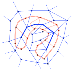
Figure 1: An example illustrating that the nodes of $X^{*}$ are on the boundary of a single face of $H^{*}$. The diagram shows part of the graph $G$ and some edges of its dual $G^{*}$. Edges of $G$ are solid blue. Edges of $P$ are bold. Dual edges are double lined red. The dual edges of $P$ are in double lined dashed red.

The procedure uses a multiple-source shortest paths (MSSP) algorithm [23, 5] to compute a table $\textrm{D}^{*}[\cdot,\cdot]$ of $X^{*}$-to-$X^{*}$ distances in $H^{*}$ with respect to the lengths $\ell(\cdot)$.

The implementation of lines 1– 10 of the abstract algorithm using the chosen representation of $\bm{f}^{\prime}$ is straightforward. We therefore focus on the implementation of line 11 of Algorithm 2, given as Algorithm 4.

Consider iteration $i$ of the algorithm. The main difference between the inefficient implementation and the efficient one is in implementing the Dijkstra step for computing shortest paths in the dual. Instead of computing the entire shortest-path tree, the procedure computes just the distance labels of nodes in $X^{*}$. This is done using the FR data structure, whose initialization requires the $X^{*}$-to-$X^{*}$ distances in $H^{*}$ with respect to the residual capacities. We now explain how these distances can be obtained.

The flow on a dart $d$ in the primal is

$$\bm{f}[d]+\boldsymbol{\phi}[\text{head}_{G^{*}}(d)]-\boldsymbol{\phi}[\text{tail}_{G^{*}}(d)].$$ (4)

Therefore the residual capacity of $d$ is

$$(\bm{c}[d]-\bm{f}[d])-\boldsymbol{\phi}[\text{head}_{G^{*}}(d)]+\boldsymbol{\phi}[\text{tail}_{G^{*}}(d)]$$ (5)

which is its reduced length $\ell_{\boldsymbol{\phi}}[d]$ with respect to the length $\ell(\cdot)$ and price function $\boldsymbol{\phi}$.

Suppose that $d$ belongs to $H^{*}$, i.e. $d$ is not one of the darts of $P\cup\mbox{rev}(P)$. The procedure never changes $\bm{f}[d]$, so $\bm{f}[d]=\bm{f}_{0}[d]$. Therefore $\ell(d)=\bm{c}[d]-\bm{f}_{0}[d]$. These lengths are known at the beginning of the procedure’s execution. The reduced length of an $X^{*}$-to-$X^{*}$ path $Q=d^{\prime}_{1},d^{\prime}_{2},\cdots,d^{\prime}_{j}$ in $H^{*}$ is

$$\sum_{i=1}^{j}\left(\ell(d^{\prime}_{i})-\boldsymbol{\phi}[\text{head}_{G^{*}}(d^{\prime}_{i})]+\boldsymbol{\phi}[\text{tail}_{G^{*}}(d^{\prime}_{i})]\right)=\left(\sum_{i=1}^{j}\ell(d^{\prime}_{i})\right)-\boldsymbol{\phi}[\mbox{end}(Q)]+\boldsymbol{\phi}[\mbox{start}(Q)].$$ (6)

Therefore, for any nodes $x,y\in X^{*}$, the $x$-to-$y$ distance in $H^{*}$ w.r.t. the residual capacity is given by $\textrm{D}^{*}[x,y]-\boldsymbol{\phi}[y]+\boldsymbol{\phi}[x]$. Since the procedure maintains the restriction of $\boldsymbol{\phi}$ to faces of $X^{*}$, this distance can be obtained in constant time. Adapting FR’s data structure to handle reduced distances w.r.t. a price function $\boldsymbol{\phi}$ was discussed in Section 3.2.1.

Algorithm 4 Efficient Implementation of line 11 of AbstractFixConservationOnPath (Algorithm 2)

1:  residual capacity $:=\bm{c}[d]-\bm{f}[d]-\boldsymbol{\phi}^{X}[\text{head}_{G^{*}}(d)]+\boldsymbol{\phi}^{X}[\text{tail}_{G^{*}}(d)]$ % push flow on $d$ to make its residual capacity zero as required for Hassin’s algorithm

2:  val $:=\min\{\text{\it residual capacity},|\bm{v}[p_{i}]|\}$ amount of flow pushed on $d$

3:  $\bm{f}[d]=\bm{f}[d]+\text{\it val}$ ; $\bm{f}[\mbox{rev}(d)]:=-\bm{f}[d]$

4:  $\bm{v}[\text{tail}(d)]=\bm{v}[\text{tail}(d)]-\text{\it val}$ ; $\bm{v}[\text{head}(d)]=\bm{v}[\text{head}(d)]+\text{\it val}$ update the inflow at $p_{i}$ and $p_{i+1}$ % push excess inflow from $\text{tail}(d)$ to $\text{head}(d)$ using Hassin’s algorithm

5:  let $\ell[d^{\prime}]:=\bm{c}[d^{\prime}]-\bm{f}[d^{\prime}]$ for all darts $d^{\prime}\in P\cup\mbox{rev}(P)$ lengths of explicit darts are residual capacities (not including circulation component)

6:  $\ell[\mbox{rev}(d)]:=|\bm{v}[p_{i}]|-\boldsymbol{\phi}^{X}[\text{tail}_{G^{*}}(\mbox{rev}(d))]+\boldsymbol{\phi}^{X}[\text{head}_{G^{*}}(\mbox{rev}(d))]$ set the limit on the residual capacity of $\mbox{rev}(d)$ (adjusted by circulation component)

7:  $\boldsymbol{\phi}_{i}^{X}(\cdot):=FR(\textrm{D}^{*},\ell,\boldsymbol{\phi}^{X},\text{head}_{G^{*}}(d))$ face potential are distances in $G^{*}$ from $\text{head}_{G^{*}}(d)$ w.r.t.  the reduced lengths induced by $\boldsymbol{\phi}^{X}$

8:  val $:=\boldsymbol{\phi}_{i}^{X}[\text{head}(d)]-\boldsymbol{\phi}_{i}^{X}[\text{tail}(d)]$ the amount of flow assigned to $d$ by the circulation corresponding to $\boldsymbol{\phi}_{i}^{X}$

9:  $\bm{f}[d]:=\bm{f}[d]-\text{\it val}$ ; $\bm{f}[\mbox{rev}(d)]:=-\bm{f}[(d)]$ do not push the circulation on $d$ and $\mbox{rev}(d)$

10:  $\boldsymbol{\phi}^{X}=\boldsymbol{\phi}^{X}+\boldsymbol{\phi}_{i}^{X}$ accumulate the current circulation

11:  $\bm{v}[\text{tail}(d)]=\bm{v}[\text{tail}(d)]-\text{\it val}$ ; $\bm{v}[\text{head}(d)]=\bm{v}[\text{head}(d)]+\text{\it val}$ update the inflow at $p_{i}$ and $p_{i+1}$

It follows from the above discussion that, after executing line 11 of Algorithm 2 using the efficient implementation (Algorithm 4) for the last time, the flow assignment $\bm{f}$ maintained by the efficient implementation is the same as the one that would have been computed if the inefficient implementation (Algorithm 3) were used. Moreover, the potential function $\boldsymbol{\phi}^{X}$ computed by the efficient implementation is the restriction to $X^{*}$ of the potential function $\boldsymbol{\phi}$ that would have been computed by the inefficient implementation.

In order to output the flow $\bm{f}^{\prime}$ in the entire graph $G$, we need to know the potential function $\boldsymbol{\phi}$ rather than just its restriction $\boldsymbol{\phi}^{X}$. Observe, however, that any pseudoflow that differs from $\bm{f}$ by a circulation is a valid output of FixConservationOnPath since a circulation does not change the inflow at any node, nor does it introduce residual paths between nodes that are not connected by a residual path in $G_{\bm{f}}$. It therefore suffices to find any feasible circulation $\boldsymbol{\chi}$ in $G_{\bm{f}}$. This can be done by computing shortest paths in $G^{*}$ w.r.t. the lengths $\ell:=\bm{c}-\bm{f}$ from an arbitrary node $x\in G^{*}$. Note, however, that for darts of $P\cup\mbox{rev}(P)$ these lengths might be negative. We therefore use the $O(n\log^{2}n/\log\log n)$-time algorithm for shortest paths with negative lengths in planar graphs [30] to compute a feasible circulation $\boldsymbol{\chi}$.  

The pseudocode for the efficient implementation of FixConservationOnPath is given in appendix D.

Running Time Analysis

Let $n$ and $k$ be the number of nodes in $G$ and in $P$, respectively. The initialization time is dominated by the $O(n\log n+k^{2}\log n)$ time for MSSP. The execution of each iteration of the main loop is dominated by the call to FR, which takes $O(k\log^{2}k)$ time. The number of iterations is $k-1$, leading to a total of $O(k^{2}\log^{2}k)$ time for execution of the main loop. Computing the circulation $\boldsymbol{\chi}$ requires one shortest path computation, which takes $O(n\log^{2}n/\log\log n)$ time. Thus total running time of the efficient implementation of FixConservationOnPath is $O(n\log^{2}n/\log\log n+k^{2}\log^{2}k)$.

4 Pushing Excess Inflow from a Cycle

In this section we describe the procedure CycleToSingleSinkLimitedMaxFlow that pushes excess inflow from a cycle to a node not on the cycle. The procedure is given as Algorithm 5. The procedure SingleSourceToCycleLimitedMaxFlow is very similar. We omit its description.

Algorithm 5 CycleToSingleSinkLimitedMaxFlow($G,\bm{c},\bm{f}_{0},C,t$)

Input: a directed planar graph $G$ with capacities $\bm{c}$, a pseudoflow $\bm{f}_{0}$, a simple cycle $C$, a sink $a_{i}$.
Assumes: $\forall v\in C^{+},\ \textrm{inflow}_{\bm{f}_{0}}(v)\geq 0$, where $C^{+}=\{v\in C:\{x\in C:\textrm{inflow}_{\bm{f}_{0}}(x)>0\}\stackrel{{\scriptstyle G_{\bm{f}_{0}}}}{{\rightarrow}}v\}$.
Output: a pseudoflow $\bm{f}$ s.t. (i) $\bm{f}-\bm{f}_{0}$ obeys conservation everywhere but $C^{+}\cup\{t\}$,
(ii) $\forall v\in C^{+},\ \textrm{inflow}_{\bm{f}}(v)\geq 0$, (iii) $\{v\in C:\textrm{inflow}_{\bm{f}}(v)>0\}\stackrel{{\scriptstyle G_{\bm{f}}}}{{\nrightarrow}}a_{i}$.

1:  let $C^{+}:=\{v\in C:\textrm{there exists a residual path to $v$ from a node }x\in C\textrm{ with }\textrm{inflow}_{\bm{f}_{0}}(x)>0\}$

2:  delete the nodes of $C-C^{+}$

3:  let $v_{1},v_{2},\dots,v_{\ell}$ be the nodes of $C^{+}$, labeled according to their cyclic order on $C$

4:  add artificial arcs $v_{i}v_{i+1}$ for $1\leq i<\ell$

5:  let $P$ be the $v_{1}$-to-$v_{\ell}$ path of artificial arcs

6:  contract all the edges of $P$, collapsing $C^{+}$ into the single node $v_{1}$

7:  $\bm{f}:=$ SingleSourceSingleSinkMaxFlow($G,\bm{c}-\bm{f}_{0},c_{1},t$)

8:  undo the contraction of the edges of $P$

9:  $\bm{f}:=$ FixConservationOnPath($G,P,\bm{c},\bm{f}_{0}+\bm{f}$) $-\bm{f}_{0}$

10:  modify $\bm{f}$ to push back flow to nodes of $C^{+}$ whose inflow w.r.t $\bm{f}_{0}+\bm{f}$ is negative

11:  $\bm{f}:=\bm{f}_{0}+\bm{f}$

12:  return  $\bm{f}$

To compute $C^{+}$ in Line 1, consider the residual graph of $G$ w.r.t. $\bm{f}_{0}$. Add a node $v$ and non-zero capacity arcs $vw$ for every node $w$ whose inflow w.r.t. $\bm{f}_{0}$ is positive (these arcs may not preserve planarity). In $O(|G|)$ time, find the set $X$ of nodes that are reachable from $v$ via darts with non-zero capacity. Then $C^{+}=C\cap X$.

Since $C^{+}$ consists of all nodes of $C$ reachable via residual paths from the nodes of $C$ with positive inflow, the flow computed by the procedure involves no darts incident to nodes in $C-C^{+}$. Thus, restricting the computation to the graph obtained from $G$ by deleting the nodes in $C-C^{+}$ (line 2) does not restrict the computed flow. After deletion, adding artificial arcs between consecutive nodes of $C^{+}$ (line 4) will not violate planarity. Contracting the artificial arcs effectively turns $C^{+}$ into a single node $v_{1}$. Next, the procedure computes a maximum flow $\bm{f}$ from $C^{+}$ to $t$ w.r.t. residual capacities $\bm{c}-\bm{f}_{0}$. This is done by invoking a single-source single-sink maximum flow algorithm [2] with source $v_{1}$ and sink $t$ (line 7). Uncontracting the artificial arcs turns $\bm{f}$ into a maximum $C^{+}$-to-$t$ flow in $G$ w.r.t. the residual capacities $\bm{c}-\bm{f}_{0}$. However, some of the nodes of $C^{+}$ may have negative inflow w.r.t. $\bm{f}_{0}+\bm{f}$. In line 9, the procedure calls FixConservationOnPath to reroute the flow $\bm{f}$ among the nodes of $C^{+}$ so that, w.r.t. $\bm{f}_{0}+\bm{f}$, there are no residual paths from nodes of $C^{+}$ with positive inflow to nodes of $C^{+}$ with negative inflow. This implies that any node of $C^{+}$ that still has negative inflow has pushed too much flow. Line 10 modifies $\bm{f}$ to push back such excess flow so that no node of $C^{+}$ has negative inflow w.r.t. $\bm{f}_{0}+\bm{f}$. This is done using the procedure of Section 1.1 described in the appendix. Finally, the procedure returns $\bm{f}_{0}+\bm{f}$. See Appendix F for a formal proof of correctness.

We next analyze the running time of this procedure on an $n$-node graph $G$ and a $k$-node cycle $C$. The $st$-maximum flow computation in line 7 takes $O(n\log n)$ time using the algorithm of Borradaile and Klein [2]. The running time of the procedure is therefore dominated by the call to FixConservationOnPath in line 9 which takes $O(n\log^{2}n/\log\log n+k^{2}\log^{2}k)$ time.

Appendix A Correctness of Algorithm 1

Lemma A.1.

Let $\bm{\rho}$ be a circulation. Let $u$ and $v$ be nodes in a graph $G$. Then

$$u\stackrel{{\scriptstyle G}}{{\nrightarrow}}v\Rightarrow u\stackrel{{\scriptstyle G_{\bm{\rho}}}}{{\nrightarrow}}v.$$

Proof.

Pushing a circulation does not change the amount of flow crossing any cut. This implies that if there was no $u$-to-$v$ residual path before $\bm{\rho}$ was pushed, then there is none after $\bm{\rho}$ is pushed. ∎

We will use the following two lemmas in the proof of correctness:

Lemma A.2.

(sources lemma) Let $f$ be a flow with source set $X$. Let $A,B$ be two disjoint sets of nodes. Then

$$A\cup X\stackrel{{\scriptstyle G}}{{\nrightarrow}}B\Rightarrow A\stackrel{{\scriptstyle G_{f}}}{{\nrightarrow}}B.$$

Proof.

The flow $f$ may be decomposed into a cyclic component (a circulation) and an acyclic component. By Lemma A.1, it suffices to show the lemma for an acyclic flow $f$.

Suppose for the sake of contradiction that there exists a residual $a$-to-$b$ simple path $P$ after $f$ is pushed for some $a\in A$ and $b\in B$. Let $P^{\prime}$ be the maximal suffix of $P$ that was residual before the push. Maximality implies that the dart $d$ of $P$ whose head is $\mbox{start}(P^{\prime})$ was non-residual before the push, and $f(\mbox{rev}(d))>0$. The fact that $f(\mbox{rev}(d))>0$ implies that before $f$ was pushed there was a residual path $Q$ from some node $x\in X$ to $\text{head}(d)$. Therefore, the concatenation of $Q$ and $P^{\prime}$ was a residual $x$-to-$b$ residual path before the push, a contradiction. ∎

The proof of the following lemma is symmetric.

Lemma A.3.

(sinks lemma) Let $f$ be a flow with sink set $X$. Let $A,B$ be two disjoint sets of nodes. Then

$$A\stackrel{{\scriptstyle G}}{{\nrightarrow}}B\cup X\Rightarrow A\stackrel{{\scriptstyle G_{f}}}{{\nrightarrow}}B.$$

For node sets $W,Y,Z$, we will use the notation sources lemma$(W,Y,Z)$ to indicate the use of the sources lemma to establish that there are no $W$-to-$Y$ residual paths after a flow with source set $Z$ is pushed. We will use sinks lemma$(W,Y,Z)$ in a similar manner.

Lemma A.4.

At any time in the running of the algorithm after the last execution of line 7 and before the execution of line 13, $S\nrightarrow T$, $S\nrightarrow A$, $S\nrightarrow C$, $A\nrightarrow T$, $C\nrightarrow T$.

Proof.

The fact that the properties hold just after line 7 follows from the properties of the recursive calls and from the fact that any residual path from a node in one piece to a node in the other consists of a residual path to $C$ and a residual path from $C$. Note that, because of the contractions in line 4, at this time the cycle $C$ consists of just the node $v$. The the nonexistence of residual paths with respect to $v$ in the recursive calls implies the nonexistence of residual paths w.r.t. any node of $C$ after the contractions are undone in line 8.

Now, let us prove that the properties are maintained until just before the execution of line 13. By the above argument, there is a cut separating $S$ from $T\cup A\cup C$ which is saturated just after line 8. The procedure in line 9 only pushes flow between vertices of $C$, and in lines 10– 12, flow is only pushed between the nodes of $A$ and $C$. These sets are all on the same side of the cut which therefore stays saturated. It follows that $S\nrightarrow T$, $S\nrightarrow A$, and $S\nrightarrow C$ at any point after line 7 and before line 13. A similar argument applied to a saturated cut separating $A\cup C$ from $T$ shows $A\nrightarrow T$ and $C\nrightarrow T$. ∎

Recall that $C_{i}^{+}$ is the set of nodes of $C$ that are reachable via residual paths from some node of $C$ with positive excess at the beginning of iteration $i$, and that $C_{i}^{-}$ is the set of nodes of $C$ that have residual paths to some node of $C$ with negative excess at the beginning of iteration $i$.

Lemma A.5.

Just after line 9 of Algorithm 1 is executed, $C_{1}^{+}\nrightarrow C_{1}^{-}$.

Proof.

Follows from the definition of FixConservationOnPath. ∎

Lemma A.6.

For all $i<j$, $C^{+}_{j}\subseteq C_{i}^{+}$ and $C^{-}_{j}\subseteq C_{i}^{-}$

Proof.

It suffices to show that, for all $i$, $C^{+}_{i+1}\subseteq C^{+}_{i}$ and $C^{-}_{i+1}\subseteq C^{-}_{i}$.

The flow pushed in iteration $i$ of line 11 can be decomposed into a flow whose sources and sinks are all in $C^{+}_{i}$ and a flow whose sources are in $C_{i}^{+}$ and whose sink is $a_{i}$. Therefore, the set $X$ of nodes of $C$ with positive inflow immediately after iteration $i$ of line 11 is a subset of $C^{+}_{i}$. By definition of SingleSourceToCycleLimitedMaxFlow, the set of nodes of $C$ with positive inflow does not change after line 12 is executed. Therefore, $C^{+}_{i+1}$ is the set of nodes reachable from $X$ by a residual path after iteration $i$ of line 12.

By definition of $C^{+}_{i}$, immediately before iteration $i$ of line 11 there are no $C^{+}_{i}$-to-$\{C-C^{+}_{i}\}$ residual paths. By sources lemma($C^{+}_{i},C-C^{+}_{i},C^{+}_{i}$), there are no $C^{+}_{i}$-to-$\{C-C^{+}_{i}\}$ residual paths immediately after iteration $i$ of line 11 as well. This shows that there are no $X$-to-$\{C-C^{+}_{i}\}$ residual paths at that time.

The flow pushed in line 12 can be decomposed into a flow whose sources and sinks are all in $C^{-}_{i}$ and a flow whose source is $a_{i}$ and whose sinks are all in $C_{i}^{-}$. By sinks lemma($C^{+}_{i},C-C^{+}_{i},C^{-}_{i}$), there are no $C^{+}_{i}$-to-$\{C-C^{+}_{i}\}$ residual paths immediately after iteration $i$ of line 12. This shows that there are no $X$-to-$\{C-C^{+}_{i}\}$ residual paths at that time. Hence $C^{+}_{i+1}\subseteq C^{+}_{i}$, as desired.

The proof of the analogous claim for $C^{-}_{i+1}$ is similar. ∎

Lemma A.7.

Just after line 11 of Algorithm 1 is executed in iteration $i$, $C_{i}^{+}\nrightarrow C_{i}^{-}$, $C_{i+1}^{+}\nrightarrow\{a_{j}\}_{j\leq i}$, $\{a_{j}\}_{j<i}\nrightarrow C_{i}^{-}$.

Proof.

The flow pushed in line 11 can be decomposed into a flow whose sources and sinks are all in $C^{+}_{i}$ and a flow whose sources are in $C_{i}^{+}$ and whose sink is $a_{i}$.

• $C_{i}^{+}\nrightarrow C_{i}^{-}$ by sources lemma($C_{i}^{+},C_{i}^{-},C^{+}_{i}$)

• $C_{i+1}^{+}\nrightarrow\{a_{j}\}_{j<i}$ by sources lemma($C_{i+1}^{+},a_{j},C^{+}_{i}$)

• $C_{i+1}^{+}\nrightarrow\{a_{i}\}$ by definition of CycleToSingleSinkLimitedMaxFlow

• $\{a_{j}\}_{j<i}\nrightarrow C_{i}^{-}$ by sources lemma($a_{j},C_{i}^{-},C^{+}_{i}$)

∎

Lemma A.8.

Just after line 12 of Algorithm 1 is executed in iteration $i$, $C_{i}^{+}\nrightarrow C_{i}^{-}$, $C_{i+1}^{+}\nrightarrow\{a_{j}\}_{j\leq i}$, $\{a_{j}\}_{j\leq i}\nrightarrow C_{i+1}^{-}$.

Proof.

The flow pushed in line 12 can be decomposed into a flow whose sources and sinks are all in $C^{-}_{i}$ and a flow whose source is $a_{i}$ and whose sinks are all in $C_{i}^{-}$.

• $C_{i}^{+}\nrightarrow C_{i}^{-}$ by sinks lemma($C_{i}^{+},C_{i}^{-},C^{-}_{i}$)

• $C_{i+1}^{+}\nrightarrow\{a_{j}\}_{j\leq i}$ by sinks lemma($C_{i+1}^{+},a_{j},C^{-}_{i}$)

• $\{a_{j}\}_{j<i}\nrightarrow C_{i+1}^{-}$ by sinks lemma($a_{j},C_{i+1}^{-},C^{-}_{i}$)

• $a_{i}\nrightarrow C_{i+1}^{-}$ by definition of SingleSourceToCycleLimitedMaxFlow

∎

Let $C^{+}(C^{-})$ denote the set of nodes in $C$ with positive (negative) inflow just before line 13 is executed.

Corollary A.9.

Just before line 13 of Algorithm 1 is executed, $C^{+}\nrightarrow C^{-},C^{+}\nrightarrow A,A\nrightarrow C^{-}$.

Lemma A.10.

The following are true upon termination:

1. $\bm{f}$ is a pseudoflow

2. $\bm{f}$ obeys conservation everywhere except at $S,T,A$

3. $S\stackrel{{\scriptstyle G_{\bm{f}}}}{{\nrightarrow}}T,S\stackrel{{\scriptstyle G_{\bm{f}}}}{{\nrightarrow}}A,A\stackrel{{\scriptstyle G_{\bm{f}}}}{{\nrightarrow}}T$.

Proof.

Since every addition to $\bm{f}$ along the algorithm respects capacities of all darts, $\bm{f}$ is a pseudoflow at all times. By induction, the only nodes that do not obey conservations after the recursive calls are those of $S,T$ and $A$. Subsequent changes to $\bm{f}$ only violate conservation on the nodes of $C$, but any such violation is eliminated in line 13. Therefore upon termination $\bm{f}$ obeys conservation everywhere except $S,T$ and $A$.

Since, by Lemma A.4 and Corollary A.9 before line 13 $C^{+}\nrightarrow A$ and $C\nrightarrow T$, the flow pushed back from $C^{+}$ in line 13 must be pushed back to $S$. Similarly, the flow pushed back to $C^{-}$ must be pushed back from $T$.

Let $f_{+}$ ($f_{-}$) be the flow pushed back from $C^{+}$ to $S$ (from $T$ to $C^{-}$) in line 13. Consider first pushing back $f_{+}$.

• $S\nrightarrow T$ by sources lemma($S,T,C^{+}$)

• $S\nrightarrow A$ by sources lemma($S,A,C^{+}$)

• $A\nrightarrow T$ by sources lemma($A,T,C^{+}$)

• $S\nrightarrow C^{-}$ by sources lemma($S,C^{-},C^{+}$)

• $A\nrightarrow C^{-}$ by sources lemma($A,C^{-},C^{+}$)

Next consider pushing $f_{-}$

• $S\nrightarrow T$ by sinks lemma($S,T,C^{-}$)

• $S\nrightarrow A$ by sinks lemma($S,A,C^{-}$)

• $A\nrightarrow T$ by sinks lemma($A,T,C^{-}$)

∎

Appendix B Correctness of Algorithm 2

Lemma B.1.

The following holds immediately after iteration $i$ of the main loop (line 3).

1. For $j\leq i,j^{\prime}>j$, if $p_{j}$ has positive inflow, there is no residual path from $p_{j}$ to $p_{j^{\prime}}$. If $p_{j}$ has negative inflow, there is no residual path from $p_{j^{\prime}}$ to $p_{j}$.

2. For $j,j^{\prime}\leq i$, if $p_{j}$ has positive inflow and $p_{j^{\prime}}$ has negative inflow then there is no $p_{j}$-to-$p_{j^{\prime}}$ residual path.

Proof.

By induction on the number of iterations $i$ of the loop. For $i=0$ the invariants are trivially satisfied.

First note that the adjustments to capacities and flow in lines 6–8 do not create any new residual paths since capacities are only reduced, and no residual capacity increases. Therefore, it suffices to argue just about the flow pushed in line 11.

Assume the invariants hold up until the beginning of the $i^{th}$ iteration. We show that the invariants hold at the end of the iteration. Suppose that $p_{i}$ has positive inflow at the end of the $i^{th}$ iteration (the case of negative inflow is similar).

1. Since the flow pushed in line 11 is limited by $|\textrm{inflow}(p_{i})|$, the fact that $p_{i}$ has positive inflow at the end implies that the flow pushed was a maximum flow from $p_{i}$ to $p_{i+1}$. Since the capacities of darts between $p_{k+1}$ and $p_{k}$ for $k>i$ are sufficiently large, the maximality of the flow implies that there are no $p_{i}$-to-$p_{k}$ residual paths for any $k>i$.

   The invariant holds for nodes $p_{j}$ with positive inflow and $j<i$ by sinks lemma($\{p_{j}\}$, $\{p_{j^{\prime}}:j^{\prime}>j\}$, $\{p_{i+1}\}$).

2. Invariant 2 holds for $j,j^{\prime}<i$ by sinks lemma( $\{p_{j}:j<i,\textrm{inflow}(p_{j})>0\}$, $\{p_{j}:j<i,\textrm{inflow}(p_{j})<0\}$, $\{p_{i+1}\}$).

   The invariant holds for $p_{i}$ by invoking the sources lemma($\{p_{i}\}$, $\{p_{j}:j<i,\textrm{inflow}(p_{j})<0\}$, $\{p_{i}\}$).

∎

Corollary B.2.

Algorithm 2 is correct

Proof.

The flow $\bm{f}^{\prime}-\bm{f}_{0}$ satisfies conservation everywhere except at nodes of $P$ since the algorithm only pushes flow between nodes of $P$. By Lemma B.1, with respect to $\bm{f}^{\prime}$, there are no residual paths from nodes of $P$ with positive inflow to nodes of $P$ with negative inflow. ∎

Appendix C Converting a Pseudoflow into a Maximum Feasible Flow

Let $\bm{f}$ be a pseudoflow in a planar graph $G$ with node set $V$, sources $S$ and sinks $T$. Let $V^{+}$ denote the set of nodes $\{v\in V-(S\cup T):\textrm{inflow}_{\bm{f}}(v)>0\}$. Similarly, let $V^{-}$ denote the set of nodes $\{v\in V-(S\cup T):\textrm{inflow}_{\bm{f}}(v)<0\}$. Suppose $S\cup V^{+}\stackrel{{\scriptstyle G_{\bm{f}}}}{{\nrightarrow}}T\cup V^{-}$. In this appendix we show how to convert $\bm{f}$ into a maximum feasible flow $\bm{f}^{\prime}$. This procedure was first described for planar graphs by Johnson and Venkatesan [19]. The original description of the procedure took $O(n\log n)$ time, but using the flow cycles canceling technique of Kaplan and Nussbaum [20] the running time is $O(n)$.

We begin by converting $\bm{f}$ to an acycic pseudoflow in linear time [20]. That is, after the conversion there is no cycle $C$ such that $\bm{f}[d]>0$ for every dart $d$ of $C$. Since $\bm{f}$ is acyclic, the darts with a positive flow induce a topological ordering on the nodes of the graph $G$. Let $v$ be the last member of $V^{+}$ in the topological ordering, and let $d$ be an arbitrary dart that carries flow into $v$. We set $\bm{f}[d]=\max\{\bm{f}[d]-\textrm{inflow}_{\bm{f}}(v),0\}$, and set $\bm{f}[\mbox{rev}(d)]$ accordingly. The flow assignment $\bm{f}$ maintains the invariant $S\cup V^{+}\stackrel{{\scriptstyle G_{\bm{f}}}}{{\nrightarrow}}T\cup V^{-}$ by sinks lemma($S\cup V^{+}$,$T\cup V^{-}$,$\{v\}$). As long as $v$ is in $V^{+}$, there must be a dart $d$ which carries flow to $v$. By changing the flow on $d$ we cannot add to $V^{+}$ a new node that appears later than $v$ in the topological ordering. We repeat this process until $V^{+}$ is empty. Since we reduce the flow on each dart at most once, this takes linear time. Next we handle $V^{-}$ while keeping the invariant $S\cup V^{+}\stackrel{{\scriptstyle G_{\bm{f}}}}{{\nrightarrow}}T\cup V^{-}$ in a symmetric way, by repeatedly fixing the first vertex if $V^{-}$ in the topological ordering.

The total running time is $O(n)$, and since $V^{+},V^{-}$ are both empty, we get from the invariant $S\cup V^{+}\stackrel{{\scriptstyle G_{\bm{f}}}}{{\nrightarrow}}T\cup V^{-}$ that the resulting pseudoflow is a feasible flow. This is the required flow $\bm{f}^{\prime}$.

Appendix D Pseudocode for FixConservationOnPath

Algorithm 6 FixConservationOnPath$(G,P,\bm{c},\bm{f}_{0})$

Input: a directed planar graph $G$, simple path $P=d_{1}d_{2}\ldots d_{k}$, capacity function $\bm{c}$, and a pseudoflow $\bm{f}_{0}$
Output: a pseudoflow $\bm{f}$ s.t. (1) $\bm{f}-\bm{f}_{0}$ satisfies conservation at nodes not on $P$ and (2) w.r.t $\bm{f}$, no residual path exists from $\{v\in P:\textrm{inflow}(v)>0\}$ to $\{v\in P:\textrm{inflow}(v)<0\}$.

1:  let $X^{*}$ be the set of endpoints in the planar dual $G^{*}$ of the darts of $P$

2:  initialize to zero an array $\boldsymbol{\phi}^{X}[\cdot]$ indexed by the nodes of $X^{*}$

3:  let $H^{*}$ be the graph obtained from $G^{*}$ by removing the darts of $P$

4:  compute, using the MSSP algorithm [23, 5], a table $\textrm{D}^{*}[\cdot,\cdot]$ of distances in $H^{*}$ between nodes of $X^{*}$ w.r.t the lengths $\bm{c}-\bm{f}_{0}$

5:  $\bm{f}:=\bm{f}_{0}$

6:  $\bm{c}[d]:=\bm{c}[d]+M$ for all darts of $P\cup\mbox{rev}(P)$

7:  initialize an array of length $k$ by $\bm{v}[i]:=$ inflow at $p_{i}$ with respect to $\bm{f}$

8:  for $i=1,2,\ldots,k$ 

9:     let $p_{i}$ and $p_{i+1}$ be the tail and head of $d_{i}$, respectively % reduce the capacities of $d$ and $\mbox{rev}(d)$ by $M$ and adjust the flow appropriately

10:     for $d\in\{d_{i},\mbox{rev}(d_{i})\}$ 

11:        $\bm{c}[d]:=\bm{c}[d]-M$

12:        $\text{\it old flow}:=\bm{f}[d]+\boldsymbol{\phi}^{X}[\text{head}_{G^{*}}(d)]-\boldsymbol{\phi}^{X}[\text{tail}_{G^{*}}(d)]$

13:        $\text{\it new flow}:=\min\{\text{\it old flow},\bm{c}[d]\}$ adjusted flow must not exceed adjusted capacity

14:        $\bm{f}[d]:=\text{\it new flow}-\boldsymbol{\phi}^{X}[\text{head}_{G^{*}}(d)]+\boldsymbol{\phi}^{X}[\text{tail}_{G^{*}}(d)]$ the explicit flow does not include the circulation component

15:        $\bm{f}[\mbox{rev}(d)]:=-\bm{f}[d]$

16:        $\bm{v}[\text{head}(d)]:=\bm{v}[\text{head}(d)]+\text{\it new flow}-\text{\it old flow}$ update the inflow at $p_{i}$ and $p_{i+1}$

17:        $\bm{v}[\text{tail}(d)]:=\bm{v}[\text{tail}(d)]-\text{\it new flow}+\text{\it old flow}$

18:     if $\bm{v}[p_{i}]>0$ then $d:=d_{i}$ else $d:=\mbox{rev}(d_{i})$ find in which direction flow should be pushed % push flow on $d$ to make its residual capacity zero as required for Hassin’s algorithm

19:     residual capacity $:=\bm{c}[d]-\bm{f}[d]-\boldsymbol{\phi}^{X}[\text{head}_{G^{*}}(d)]+\boldsymbol{\phi}^{X}[\text{tail}_{G^{*}}(d)]$

20:     val $:=\min\{\text{\it residual capacity},|\bm{v}[p_{i}]|\}$ amount of flow pushed on $d$

21:     $\bm{f}[d]=\bm{f}[d]+\text{\it val}$ ; $\bm{f}[\mbox{rev}(d)]:=-\bm{f}[d]$

22:     $\bm{v}[\text{tail}(d)]=\bm{v}[\text{tail}(d)]-\text{\it val}$ ; $\bm{v}[\text{head}(d)]=\bm{v}[\text{head}(d)]+\text{\it val}$ update the inflow at $p_{i}$ and $p_{i+1}$ % push excess inflow from $\text{tail}(d)$ to $\text{head}(d)$ using Hassin’s algorithm

23:     let $\ell[d^{\prime}]:=\bm{c}[d^{\prime}]-\bm{f}[d^{\prime}]$ for all darts $d^{\prime}\in P\cup\mbox{rev}(P)$ lengths of explicit darts are residual capacities (not including circulation component)

24:     $\ell[\mbox{rev}(d)]:=|\bm{v}[p_{i}]|-\boldsymbol{\phi}^{X}[\text{tail}_{G^{*}}(\mbox{rev}(d))]+\boldsymbol{\phi}^{X}[\text{head}_{G^{*}}(\mbox{rev}(d))]$ set the limit on the residual capacity of $\mbox{rev}(d)$ (adjusted by circulation component)

25:     $\boldsymbol{\phi}_{i}^{X}(\cdot):=FR(\textrm{D}^{*},\ell,\boldsymbol{\phi}^{X},\text{head}_{G^{*}}(d))$ face potential are distances in $G^{*}$ from $\text{head}_{G^{*}}(d)$ w.r.t.  the reduced lengths induced by $\boldsymbol{\phi}^{X}$

26:     val $:=\boldsymbol{\phi}_{i}^{X}[\text{head}(\mbox{rev}(d))]-\boldsymbol{\phi}_{i}^{X}[\text{tail}(\mbox{rev}(d))]$ the amount of flow assigned to $d$ by the circulation corresponding to $\boldsymbol{\phi}_{i}^{X}$

27:     $\bm{f}[d]:=\bm{f}[d]+\text{\it val}$ ; $\bm{f}[\mbox{rev}(d)]:=-\bm{f}[(d)]$ do not push the circulation on $d$ and $\mbox{rev}(d)$

28:     $\boldsymbol{\phi}^{X}=\boldsymbol{\phi}^{X}+\boldsymbol{\phi}_{i}^{X}$ accumulate the current circulation

29:     $\bm{v}[\text{tail}(d)]=\bm{v}[\text{tail}(d)]-\text{\it val}$ ; $\bm{v}[\text{head}(d)]=\bm{v}[\text{head}(d)]+\text{\it val}$ update the inflow at $p_{i}$ and $p_{i+1}$ % find a feasible circulation

30:  let $x$ be an arbitrary node in $G^{*}$

31:  let $\ell[d]:=\bm{c}[d]-\bm{f}[d]$ for all darts $d\in G$

32:  $\boldsymbol{\chi}:=\textnormal{SingleSourceShortestPaths}(G^{*},\ell,x)$ distances of the nodes of $G^{*}$ from $x$

33:  $\bm{f}^{\prime}[d]:=\bm{f}[d]+\boldsymbol{\chi}[\text{head}_{G^{*}}(d)]-\boldsymbol{\chi}[\text{tail}_{G^{*}}(d)]$ for every dart $d\in G$ add explicit flow and implicit circulation

34:  return  $\bm{f}^{\prime}$

Appendix E Alternative to Line 32 of Algorithm 6

In this section we show that it is not necessary to use a generic shortest path algorithm that works with negative lengths to compute a feasible circulation $\boldsymbol{\chi}$ in line 32 of Algorithm 6. Instead of choosing $x$ to be an arbitrary node in $G^{*}$, let $x$ be an arbitrary node of $X^{*}$. Let $\boldsymbol{\chi}(y)$ denote the $x$-to-$y$ distance in $G^{*}$ w.r.t. the lengths $\ell$. Instead of computing $\boldsymbol{\chi}$ using a shortest path algorithm that accepts negative lengths, we will compute it more efficiently in two steps. Pseudocode is given below as Algorithm 7. In the first step we use FR to compute the distances to just the nodes of $X^{*}$. In the second step we extend these distances to all other nodes using Dijkstra’s algorithm.

In the first step the algorithm computes distances in $G^{*}$ from $x$ to all nodes of $X^{*}$ w.r.t. $\ell_{\boldsymbol{\phi}^{X}}$, the reduced lengths of $\ell$ induced by the feasible price function $\boldsymbol{\phi}^{X}$. This is done by an additional invocation of FR (line 2). Let $\boldsymbol{\psi}^{X}$ denote these distance labels. By definition of reduced lengths and a telescoping sum similar to the one in the derivation of Eq. (6),

$$\boldsymbol{\psi}^{X}[y]=\boldsymbol{\chi}(y)+\boldsymbol{\phi}^{X}[x]-\boldsymbol{\phi}^{X}[y].$$ (7)

Since both $\boldsymbol{\phi}^{X}$ and $\boldsymbol{\psi}^{X}$ are known, the algorithm can compute the unreduced distances $\boldsymbol{\chi}[y]$ for all $y\in X^{*}$ (line 4). Next, the algorithm runs Dijkstra’s algorithm on $G^{*}$, initializing the label of each node $y$ of $X^{*}$ to its correct value $\boldsymbol{\chi}[y]$. Since in the dual the darts of $P\cup\mbox{rev}(P)$ are only incident to nodes of $X^{*}$, Dijkstra’s algorithm initialized in this manner correctly outputs the distance labels for all nodes of $G^{*}$ even if some of the darts of $P\cup\mbox{rev}(P)$ may have negative lengths.

Algorithm 7 Alternative to line 32 of Algorithm 6

1:  let $x$ be an arbitrary node in $X^{*}$

2:  $\boldsymbol{\psi}^{X}=FR(\textrm{D}^{*},\ell,\boldsymbol{\phi}^{X},x)$ find distances of the nodes of $X^{*}$ from $x$ w.r.t. price function $\boldsymbol{\phi}^{X}$

3:  initialize to $\infty$ an array $\boldsymbol{\chi}$ indexed by the nodes of $G^{*}$

4:  $\boldsymbol{\chi}[y]=\boldsymbol{\psi}^{X}[y]-\boldsymbol{\phi}^{X}[x]+\boldsymbol{\phi}^{X}[y]$ for every $y\in X^{*}$ distances of the nodes of $X^{*}$ from $x$

5:  extend $\ell$ to all darts of $G^{*}$ by $\ell[d]:=\bm{c}[d]-\bm{f}_{0}[d]$ for every dart $d\in G$

6:  $\boldsymbol{\chi}:=\textnormal{Dijkstra}(G^{*},\ell,x,\boldsymbol{\chi})$ distances of the nodes of $G^{*}$ from $x$

Appendix F Correctness of Algorithm 5

Lemma F.1.

Algorithm 5 is correct.

Proof.

Any flow that is pushed by the algorithm originates at $C^{+}$ and terminates at $C^{+}\cup\{t\}$. Therefore, $\bm{f}-\bm{f}_{0}$ violates conservation only at $C^{+}\cup\{t\}$. In line 10, flow of $\bm{f}$ is pushed back so that no node of $C^{+}$ has negative inflow w.r.t. $\bm{f}_{0}+\bm{f}$. It is possible to do so by only pushing back flow of $\bm{f}$ (rather than flow of $\bm{f}_{0}+\bm{f}$) since by assumption no node of $C^{+}$ has negative inflow w.r.t. $\bm{f}_{0}$.

By maximality of the flow pushed in line 7, just after line 7 is executed there are no $C^{+}$-to-$t$ residual paths. Clearly, this remains true when the capacities of the artificial darts are set to zero. In line 9 flow is pushed among the nodes of $C^{+}$, so by sources lemma($C^{+},t,C^{+}$), there are no $C^{+}$-to-$t$ residual paths after line 9 either. Moreover, by definition of FixConservationOnPath, there are no $C_{>0}$-to-$C_{<0}$ residual paths immediately after line 9 is executed, where $C_{>0}$ ($C_{<0}$) is the set of nodes of $C^{+}$ with positive (negative) inflow at that time. Line 10 pushes flow into $C_{<0}$, making all the nodes of $C_{<0}$ obey conservation. By sinks lemma($C_{>0},t,C_{<0}$) there are no $C_{>0}$-to-$t$ residual paths upon termination of the procedure. This completes the proof since $C_{>0}$ is the set of nodes of $C$ with positive inflow upon termination. ∎

References

- [1] R. Ahuja, Ö. Ergun, J. Orlin, and A. Punnen. A survey of very large scale neighborhood search techniques. Discrete Applied Mathematics, 23:75–102, 2002.
- [2] G. Borradaile and P. N. Klein. An algorithm for maximum -flow in a directed planar graph. Journal of the ACM, 56(2), 2009.
- [3] Y. Boykov and V. Kolmogorov. An experimental comparison of min-cut/max-flow algorithms for energy minimization in vision. IEEE Transactions on Pattern Analysis and Machine Intelligence, 26(9):1124–1137, 2004.
- [4] Y. Boykov, O. Veksler, and R. Zabih. Efficient approximate energy minimization via graph cuts. IEEE Transactions on Pattern Analysis and Machine Intelligence, 20(12):1222–1239, 2001.
- [5] S. Cabello and E. W. Chambers. Multiple source shortest paths in a genus graph. In Proceedings of the 18th Annual ACM-SIAM Symposium on Discrete Algorithms, pages 89–97, 2007.
- [6] M. de Berg, M. van Kreveld, M. Overmars, and O. Schwarzkopf. Computational Geometry: Algorithms and Applications. Springer-Verlag, 2nd edition edition, 2000. pp. 96–99.
- [7] J. Erickson. Maximum flows and parametric shortest paths in planar graphs. In Proceedings of the 21st Annual ACM-SIAM Symposium on Discrete Algorithms, pages 794–804, 2010.
- [8] J. Fakcharoenphol and S. Rao. Planar graphs, negative weight edges, shortest paths, and near linear time. Journal of Computer and System Sciences, 72(5):868–889, 2006.
- [9] S. Geman and D. Geman. Stochastic relaxation, Gibbs distributions, and the Bayesian relation of images. IEEE Transactions on Pattern Analysis and Machine Intelligence, 6(6):721–742, 1984.
- [10] A. Goldberg and S. Rao. Beyond the flow decomposition barrier. Journal of the ACM, 45(5):783–797, 1998.
- [11] A. V. Goldberg and R. E. Tarjan. Solving minimum-cost flow problems by successive approximation. In Proceedings of the 19th Annual ACM Symposium on Theory of Computing, pages 7–18, 1987.
- [12] D. Greig, B. Porteous, and A. Seheult. Exact maximum a posteriori estimation for binary images. Journal of the Royal Statistical Society, Series B, 51(2):271–279, 1989.
- [13] R. Hassin. Maximum flow in planar networks. Information Processing Letters, 13(3):107, 1981.
- [14] M. R. Henzinger, P. N. Klein, S. Rao, and S. Subramanian. Faster shortest-path algorithms for planar graphs. Journal of Computer and System Sciences, 55(1):3–23, 1997.
- [15] D. S. Hochbaum. An efficient algorithm for image segmentation, Markov random fields and related problems. Journal of the ACM, 48(4):686–701, 2001.
- [16] D. S. Hochbaum. The pseudoflow algorithm: A new algorithm for the maximum-flow problem. Operations Research, 56(4):992–1009, 2008.
- [17] G. F. Italiano, Y. Nussbaum, P. Sankowski, and C. Wulff-Nilsen. Improved algorithms for min cut and max flow in undirected planar graphs. In Proceedings of the 43rd Annual ACM Symposium on Theory of Computing, 2011. To appear.
- [18] D. B. Johnson. Efficient algorithms for shortest paths in sparse networks. Journal of the ACM, 24(1):1–13, 1977.
- [19] D. B. Johnson and S. Venkatesan. Using divide and conquer to find flows in directed planar networks in time. In Proceedings of the 20th Annual Allerton Conference on Communication, Control, and Computing, pages 898–905, 1982.
- [20] H. Kaplan and Y. Nussbaum. Maximum flow in directed planar graphs with vertex capacities. In Proceedings of the 17th European Symposium on Algorithms, pages 397–407, 2009.
- [21] H. Kaplan and M. Sharir. Finding the maximal empty rectangle containing a query point. manuscript, 2011.
- [22] S. Khuller, J. Naor, and P. Klein. The lattice structure of flow in planar graphs. SIAM Journal on Discrete Mathematics, 6(3):477–490, 1993.
- [23] P. N. Klein. Multiple-source shortest paths in planar graphs. In Proceedings of the 16th Annual ACM-SIAM Symposium on Discrete Algorithms, pages 146–155, 2005.
- [24] P. N. Klein, S. Mozes, and O. Weimann. Shortest paths in directed planar graphs with negative lengths: A linear-space -time algorithm. ACM Transactions on Algorithms, 6(2):1–18, 2010.
- [25] P. N. Klein and S. Subramanian. A fully dynamic approximation scheme for shortest paths in planar graphs. Algorithmica, 22(3):235–249, 1998.
- [26] J. Kleinberg and E. Tardos. Approximation algorithms for classification problems with pairwise relationships: Metric labeling and Markov random fields. In Proceedings of the 40th Annual Symposium on Foundations of Computer Science, 1999.
- [27] P. Kohli and P. H. S. Torr. Dynamic graph cuts for efficient inference in Markov random fields. IEEE Transactions on Pattern Analysis and Machine Intelligence, 29(12):2079–2088, 2007.
- [28] G. L. Miller. Finding small simple cycle separators for 2-connected planar graphs. Journal of Computer and System Sciences, 32(3):265–279, 1986.
- [29] G. L. Miller and J. Naor. Flow in planar graphs with multiple sources and sinks. SIAM Journal on Computing, 24(5):1002–1017, 1995. Preliminary version in FOCS 1989.
- [30] S. Mozes and C. Wulff-Nilsen. Shortest paths in planar graphs with real lengths in time. In Proceedings of the 18th European Symposium on Algorithms, pages 206–217, 2010.
- [31] F. R. Schmidt, E. Toeppe, and D. Cremers. Efficient planar graph cuts with applications in computer vision. In Proceedings of the IEEE Computer Society Conference on Computer Vision and Pattern Recognition, pages 351–356, 2009.
- [32] D. D. Sleator and R. E. Tarjan. A data structure for dynamic trees. Journal of Computer and System Sciences, 26(3):362–391, 1983.
- [33] S. Subramanian. Parallel and Dynamic Shortest-Path Algorithms for Sparse Graphs. PhD thesis, Brown University, 1995. Available as Brown University Computer Science Technical Report CS-95-04.