Anharmonic resonances with recursive delay feedback

Abstract

We consider application of time-delayed feedback with infinite recursion for control of anharmonic (nonlinear) oscillators subject to noise. In contrast to the case of a single delay feedback, recursive delay feedback exhibits resonances between feedback and nonlinear harmonics, leading to a resonantly strong or weak oscillation coherence even for a small anharmonicity. Remarkably, these small-anharmonicity induced resonances can be stronger than the harmonic ones. Analytical results are confirmed numerically for van der Pol and van der Pol–Duffing oscillators.

1 Introduction

Delayed feedback is an effective control tool for chaotic and stochastic dynamics of solely oscillatory systems [1, 2, 3, 4, 5, 6, 7] and collective dynamics of ensembles of oscillators [8, 9, 10, 11]. For a recursive delay feedback (or “extended delay feedback”) the forcing on the system at the time moment $t$ is determined not merely by the state difference ${\bf z}(t)=[{\bf x}(t-\tau)-{\bf x}(t)]$ ($\tau$ is the delay time) but by a chain of differences ${\bf z}(t)=\sum_{n=0}^{+\infty}R^{n}[{\bf x}(t-(n+1)\tau)-{\bf x}(t-n\tau)]$ with $|R|<1$ [12, 13]. The employment of such a feedback can provide new opportunities in comparison to the case of the “single delay feedback” control [12, 13, 14, 15]. Moreover, the feedback has such a form when the system is connected to a resonator (for instance, an optical delayed feedback for lasers is realized with a Fabry -Perot interferometer). A recursive delay feedback is also constructively inherent to some electronic devises (e.g. [16]). It is noteworthy that, from the mathematical perspective, the infinite recursion is equivalent to the addition of the neutral equation ${\bf s}(t)=R{\bf s}(t-\tau)+{\bf x}(t-\tau)$ (then the feedback signal ${\bf z}(t)={\bf s}(t)-{\bf x}(t)$). Properties of this neutral equation provide favourable conditions for resonant phenomena in the system.

For limit-cycle oscillators subject to noise, the regularity of dynamics is characterized by oscillation coherence [17] and “reliability” [18]. Coherence can be quantified by the diffusion constant of the oscillation phase $\varphi(t)$. While for vanishing noise the phase grows linearly with time, noise results in random excursions of the phase around the average growth trend, $\langle[\varphi(t)-\varphi(0)-\langle\dot{\varphi}\rangle t]^{2}\rangle\approx Dt$, where $D$ is the diffusion constant. The “reliability” is the ability of a system to provide one and the same response for the noise signal of a prerecorded waveform. Mathematically, reliability means stability of a system response and can be measured by the Lyapunov exponent [19, 20, 21, 22, 23]. The effect of a control on the dynamics regularity can be, therefore, tracked with the phase diffusion constant and the Lyapunov exponent.

The employment of single and/or recursive delay feedback control received previously analytical treatments only for the case of a harmonic oscillator [3, 7, 15]. In this Letter, the analytical treatment is generalized for anharmonic oscillators. Strong anharmonic resonances are revealed even for a relatively small anharmonicity.

The paper is organized as follows. In Sec. 2 we derive algebraic equations for the mean frequency, the diffusion constant, and the Lyapunov exponent for general limit-cycle oscillator subject to noise and a general linear feedback represented in terms of a Green’s function. In Sec. 3 we consider the form of these equations specific to a recursive delay feedback and treat the role of anharmonicity. The analytical theory we construct is applied to van der Pol and van der Pol–Duffing oscillators. The anharmonic resonances are also observed with a direct numerical simulation. Finally, conclusions are summarized in Sec. 4.

2 Phase description

Let us consider an $N$-dimensional limit-cycle oscillator subject to recursive delay feedback and noise:

$$\dot{x}_{i}=F_{i}({\bf x})+a\,z_{i}(t)+B_{i}({\bf x})\circ\xi(t),$$ (1)

where $i=1,2,...,N$, $a$ is the feedback strength, $az_{i}(t)$ is the feedback term, $\xi(t)$ is white Gaussian noise, $\langle\xi\rangle=0$ and $\langle\xi(t)\xi(t^{\prime})\rangle=2\delta(t-t^{\prime})$, “$\circ$” indicates the Stratonovich form of stochastic equation. For briefness, we will first keep the feedback term in a general form valid for any linear feedback (as in Refs. [24, 25])

$$z_{i}(t)=\int\limits_{0}^{+\infty}\sum_{j=1}^{N}G_{ij}(t_{1})\,x_{j}(t-t_{1})\,dt_{1}\,,$$

involving Green’s function $G_{ij}(t)$; for recursive time-delayed feedback

$${\bf\hat{G}}(t)=2{\bf\hat{S}}\sum\limits_{n=0}^{+\infty}\!R^{n}\big{[}\delta(t-(n+1)\tau)-\delta(t-n\tau-0)\big{]}\quad$$

$$=2{\bf\hat{S}}\Bigg{[}-\delta(t-0)+(1-R)\sum\limits_{n=1}^{+\infty}\!R^{n-1}\delta(t-n\tau)\Bigg{]}\,,$$ (2)

where ${\bf\hat{S}}$ is a constant matrix, $\tau$ is the delay time, $|R|<1$, and we explicitly indicate that $\int_{0}^{+\infty}\delta(t-0)\,dt=1$.

For a noise-free limit-cycle oscillator, the oscillation phase $\varphi=\varphi({\bf x})$ can be introduced on the limit cycle ${\bf x}_{0}(t)={\bf x}_{0}(t+T_{0})$ and within its finite vicinity in such a way that $\dot{\varphi}=\Omega_{0}=2\pi/T_{0}$, where $\Omega_{0}$ is the natural frequency of the oscillator [26, 27]. The limit cycle can be parameterized with the phase, ${\bf x}_{0}(\varphi)={\bf x}_{0}(\varphi+2\pi)$. In the presence of a weak forcing (noise and feedback) the phase description can be still utilized;

$$\dot{\varphi}=\Omega_{0}+a\int\limits_{0}^{+\infty}\sum_{i=1}^{N}\sum_{j=1}^{N}G_{ij}(t_{1})\,H_{ij}\big{(}\varphi(t-t_{1}),\varphi(t)\big{)}\,dt_{1}$$

$$+\varepsilon f\big{(}\varphi(t)\big{)}\circ\xi(t)\,,\quad$$ (3)

where

$$f(\varphi_{1}):=\sum_{j=1}^{N}\left(\frac{\partial\varphi({\bf x})}{\partial x_{j}}B_{j}\right)_{{\bf x}={\bf x}_{0}(\varphi_{1})}$$

is a $2\pi$-periodic function featuring the sensitivity of the phase to noise, $\varepsilon$ is the noise amplitude, $H_{ij}(\psi,\varphi)$ is the increase of the phase growth rate created by the feedback term $x_{j}(\psi)$ acting on the variable $x_{i}(\varphi)$;

$$H_{ij}(\psi,\varphi_{1}):=\left.\frac{\partial\varphi({\bf x})}{\partial x_{i}}\right|_{{\bf x}={\bf x}_{0}(\varphi_{1})}x_{j}(\psi)\,.$$

Notice, accurate derivation of Eq. (3) [28, 29, 30] yields a drift term $\propto\varepsilon^{2}$, which represents the role of the amplitude degrees of freedom. Since Eq. (3) provides a noise-induced mean frequency shift $\propto\varepsilon^{2}$, i.e., of the same order of magnitude, this omitted term should be accounted for, when one considers the effect of noise on the mean frequency. However, for robustness quantifiers (the phase diffusion constant and the Lyapunov exponent, which are of our interest here) this term has been shown to be negligible [30].

For weak noise, the linear in noise approximation is relevant and yields (see Appendix for detail) the mean frequency

$$\Omega=\Omega_{0}+a\int_{0}^{+\infty}\sum_{i=1}^{N}\sum_{j=1}^{N}G_{ij}(t)\,h_{ij}(-\Omega t)\,dt\,,$$ (4)

the phase diffusion constant

$$D=\frac{2\varepsilon^{2}\langle{f^{2}}\rangle_{\varphi}}{\Big{(}1+a\int\limits_{0}^{+\infty}t\sum\limits_{i=1}^{N}\sum\limits_{j=1}^{N}G_{ij}(t)\,h^{\prime}_{ij}(-\Omega t)\,dt\Big{)}^{2}}\quad$$

$$=2\varepsilon^{2}\langle{f^{2}}\rangle_{\varphi}\left(\frac{\partial\Omega}{\partial\Omega_{0}}\right)^{2},$$ (5)

and the leading Lyapunov exponent

$$\lambda=-\frac{\varepsilon^{2}\langle(f^{\prime})^{2}\rangle_{\varphi}}{\Big{(}1+a\int\limits_{0}^{+\infty}t\sum\limits_{i=1}^{N}\sum\limits_{j=1}^{N}G_{ij}(t)\,h^{\prime}_{ij}(-\Omega t)\,dt\Big{)}^{2}}\quad$$

$$=-\varepsilon^{2}\langle(f^{\prime})^{2}\rangle_{\varphi}\left(\frac{\partial\Omega}{\partial\Omega_{0}}\right)^{2},$$ (6)

where $\langle...\rangle_{\varphi}\equiv(2\pi)^{-1}\int_{0}^{2\pi}...d\varphi$,

$$h_{ij}(\psi):=\langle H_{ij}(\varphi+\psi,\varphi)\rangle_{\varphi},$$

is the average susceptibility of the phase to the feedback term $x_{j}(\varphi+\psi)$ acting on $x_{i}(\varphi)$ (notice, this means a phase delay by $-\psi$), and the prime denotes derivative. Eq. (4) can be solved with respect to $\Omega$, and then, with $\Omega$ evaluated, Eqs. (5) and (6) provide $D$ and $\lambda$. Noticeable constancy of the ratio

$$\frac{-\lambda}{D}=\frac{\langle(f^{\prime})^{2}\rangle}{2\langle{f^{2}}\rangle}$$

was already discussed in the literature [7, 25, 6]. Henceforth, we do not consider $\lambda$ because considering the diffusion constant is enough.

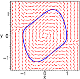
(a)  (b)
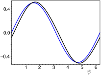
(c)
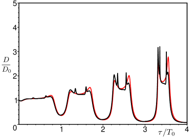
(d)

Figure 1: Van der Pol oscillator (7) with $\mu=0.7$ subject to the recursive delay feedback control. (a): The phase portrait of the system without noise and control. (b): The function of susceptibility to feedback $h_{22}(\psi)$ (black curve) and its harmonic part (blue curve). (c): The analytical dependence of the phase diffusion constant on the delay time $\tau$ (black curve) and the harmonic-approximation version of this dependence (red curve) for $R=0.5$ and $a=0.1$ ($D_{0}$ and $T_{0}\approx 2\pi/0.97$ are the diffusion constant and the mean oscillation period of the control-free system, respectively). (d): Results of a direct numerical simulation with $R=0.5$, $a=0.1$, noise strength $\varepsilon=0.02$.

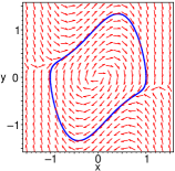
(a)  (b)
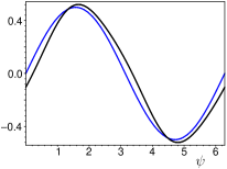
(c)
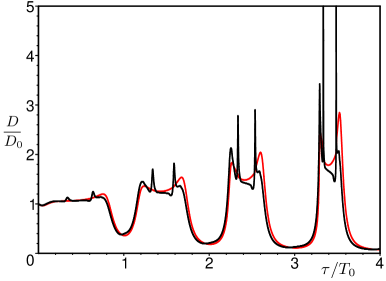
(d)

Figure 2: Van der Pol oscillator (7) with $\mu=1.0$ subject to the recursive delay feedback control. (a): The phase portrait of the control-free noiseless system. (b): $h_{22}(\psi)$. (c): Analytical dependence $D(\tau)$ ($T_{0}\approx 2\pi/0.94$). (d): Numerical simulation. For detail see caption to Fig. 1.

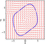
(a)  (b)

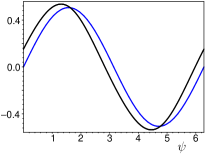
(c)

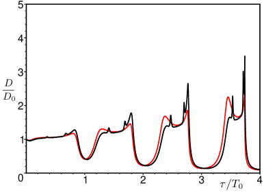
Figure 3: Van der Pol–Duffing oscillator (14) with $\mu=0.7$ and $b=0.5$ subject to the recursive delay feedback control. (a): The phase portrait of the control-free noiseless system. (b): $h_{22}(\psi)$. (c): Analytical dependence $D(\tau)$ ($T_{0}\approx 2\pi/1.14$). For detail see caption to Fig. 1.

3 Recursive delay feedback control for harmonic and anharmonic oscillators

3.1 Harmonic oscillator

Previous analytical considerations were focused on the case of a nearly harmonic oscillators [3, 7, 15, 24], such as the van der Pol one;

$$\dot{x}=y,\quad\dot{y}=\mu(1-4x^{2})y-x+az(t)+\varepsilon\,\xi(t)$$ (7)

with $\mu\ll 1$ ($\mu$ characterizes closeness to the Hopf bifurcation point). For $\mu\ll 1$, the phase $\varphi=-\arctan(y/x)$ and the limit cycle is: $x_{0}=\cos\varphi$, $y_{0}=-\sin\varphi$; therefore, the equations for $H_{ij}(\psi,\varphi)$ and $f(\varphi)$ yield

$${\bf\hat{h}}(\psi)=\left[\begin{array}[]{cc}\frac{1}{2}\sin\psi&\frac{1}{2}\cos\psi\\[5.0pt] -\frac{1}{2}\cos\psi&\frac{1}{2}\sin\psi\end{array}\right]\,,\quad f(\varphi)=-\sin\varphi\,.$$

The recursive delay feedback $az(t)$ is typically implemented in the form

$$z(t)=2\sum_{n=0}^{+\infty}R^{n}\big{(}y(t-(n+1)\tau)-y(t-n\tau)\big{)}\,,$$ (8)

which means

$${\bf\hat{S}}=\left[\begin{array}[]{cc}0&0\\ 0&1\end{array}\right],$$

as we have only the $y$-variable acting on $\dot{y}$ (compare Eq. (7) and Eqs. (1), (2)), and with $h_{22}(\psi)=(1/2)\sin\psi$ one obtains for a harmonic oscillator (cf [15])

$$\Omega=\Omega_{0}-a\frac{(1-R)\sin{\Omega\tau}}{1+R^{2}-2R\cos{\Omega\tau}}\,,$$ (9)

$$D=\frac{D_{0}}{\left(\displaystyle 1+a\tau(1-R)\frac{(1+R^{2})\cos{\Omega\tau}-2R}{(1+R^{2}-2R\cos{\Omega\tau})^{2}}\right)^{2}}\,,$$ (10)

where $D_{0}=2\varepsilon^{2}\langle{f^{2}}\rangle_{\varphi}$ is the phase diffusion constant of the control-free system.

3.2 Anharmonic oscillator

Generally, oscillators are anharmonic and $h_{22}(\psi)$ has additional terms, not only $\sin\psi$. Let us consider $h_{22}(\psi)$ in the form of a Fourier series;

$$h_{22}(\psi)=\sum_{m=1}^{\infty}(\alpha_{m}\sin{m\psi}+\beta_{m}\cos{m\psi})\,.$$ (11)

Notice, the term $\beta_{1}\cos\psi$ belongs to the first harmonic of the series as well as $\alpha_{1}\sin\psi$, but it is owed to anharmonicity; for harmonic oscillations $h_{22}(\psi)$ is purely proportional to $\sin\psi$.

With Eq. (11), Eqs. (4) and (5) take the form

$$\Omega=\Omega_{0}$$

$$-2a\sum_{m=1}^{\infty}\frac{\alpha_{m}(1-R)\sin{m\Omega\tau}+\beta_{m}(1+R)(1-\cos{m\Omega\tau})}{1+R^{2}-2R\cos{m\Omega\tau}},$$ (12)

$$D=D_{0}\Bigg{[}1+2a\,m\,\tau\,(1-R)$$

$$\times\sum_{m=1}^{\infty}\frac{\alpha_{m}[(1+R^{2})\cos{m\Omega\tau}-2R]+\beta_{m}(1-R^{2})\sin{m\Omega\tau}}{(1+R^{2}-2R\cos{m\Omega\tau})^{2}}\Bigg{]}^{-2}\!\!.$$

(13)

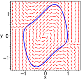
(a)  (b)

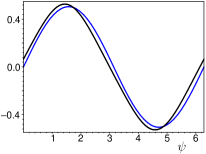
(c)

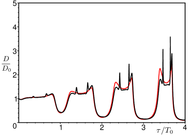
Figure 4: Van der Pol–Duffing oscillator (14) with $\mu=1.0$ and $b=0.5$ subject to the recursive delay feedback control. (a): The phase portrait of the control-free noiseless system. (b): $h_{22}(\psi)$. (c): Analytical dependence $D(\tau)$ ($T_{0}\approx 2\pi/1.12$). For detail see caption to Fig. 1.

Table 1: Fourier coefficients of $h_{22}(\varphi)$, Eq. (11), for a van der Pol–Duffing oscillator (14) ($b=0$ corresponds to a van der Pol oscillator).

	$b=0$,  $\mu=0.7$		$b=0$,  $\mu=1.0$		$b=0.5$,  $\mu=0.7$		$b=0.5$,  $\mu=1.0$
	$\alpha_{m}$	$\beta_{m}$	$\alpha_{m}$	$\beta_{m}$	$\alpha_{m}$	$\beta_{m}$	$\alpha_{m}$	$\beta_{m}$
$m=1$	$+0.501700$	$-0.076145$	$+0.499449$	$-0.093296$	$+0.506334$	$+0.153265$	$+0.505712$	$+0.070064$
$m=2$	$0$	$0$	$0$	$0$	$0$	$0$	$0$	$0$
$m=3$	$-0.010249$	$-0.003886$	$-0.018180$	$-0.010697$	$-0.009246$	$-0.001205$	$-0.015938$	$-0.005048$
$m=4$	$0$	$0$	$0$	$0$	$0$	$0$	$0$	$0$
$m=5$	$+0.000044$	$+0.000084$	$+0.000035$	$+0.000422$	$+0.000050$	$-0.000003$	$+0.000149$	$+0.000107$

3.3 Anharmonic resonances

Denominators in the sums in Eqs. (12) and (13) have extreme values for $\cos{m\Omega\tau}=\pm 1$. For a single delay, $R=0$, they equals $1$, while even for moderate values of $R$ the minima of the denominator can be close to zero. Remarkably, at points of these resonances ($\cos{m\Omega\tau}=\pm 1$) contribution of the $m$th harmonic can be large even when $\alpha_{m}$ and $\beta_{m}$ are relatively small. For instance, next to $\tau$ such that $|\cos{3\Omega\tau}|=1$, but $|\cos{\Omega\tau}|\neq 1$, one can expect resonantly strong or weak phase diffusion, due to anharmonicity.

For the demonstration and invigoration of the analytical findings, we have considered a van der Pol–Duffing oscillator:

$$\dot{x}=y,\quad\dot{y}=\mu(1-4x^{2})y-x-bx^{3}+az(t)+\varepsilon\,\xi(t)\,,$$ (14)

where $b$ is the Duffing parameter, $b=0$ corresponds to a van der Pol oscillator (7); feedback term $az(t)$ is given by Eq. (8).

For this oscillator, $h_{22}(\psi)$ and its Fourier transform (11) were calculated. Figs. 1–4 present samples of limit cycles (a) and functions $h_{22}(\psi)$ (b); the corresponding Fourier coefficients $\alpha_{m}$ and $\beta_{m}$ are provided in Tab. 1. (Interested readers can find a Maple program with comprehensive calculations in the supplementary material.) One can see in the table, that typical values of higher harmonics are small: $\alpha_{3}$ and $\beta_{3}$ are only a few percent of $\alpha_{1}\approx 1/2$. Nevertheless, the dependence $D(\tau)$ exhibits large peaks related to the $m=3$ resonances (in Figs. 1–4 these dependencies are plotted for $R=0.5$). The results of calculations without higher harmonics are plotted with red curves and can be compared to the one of the “all-harmonics” calculation; resonant discrepancies can be clearly seen. In particular, the $m=3$ resonances are even stronger than the harmonic ones related to $m=1$. The results of a direct numerical simulation show these peaks as well (Figs. 1d and 2d) and are in a good agreement with the analytical dependencies.

4 Conclusion

We have considered limit-cycle oscillators subject to weak white Gaussian noise and recursive delay feedback control. In this way, we have derived the phase reduction equation and calculated analytically the mean frequency, the phase diffusion constant, and the Lyapunov exponent (Eqs. (4)–(6)) for the case of a general linear feedback (“single” and recursive delay feedback, linear frequency filter, etc.) and a general limit-cycle oscillator.

It has been found that even a small anharmonicity leads to additional resonances and resonantly strong or weak coherence (measured by the phase diffusion constant). For instance, for van der Pol and van der Pol–Duffing oscillators, the anharmonic resonances due to the harmonic $h_{22}^{(3)}(\psi)=\alpha_{3}\sin{3\psi}+\beta_{3}\cos{3\psi}$ are even stronger than the harmonic resonances due to $h_{22}^{(\mathrm{harm})}(\psi)=(1/2)\sin\psi$ (Fig. 1–4). Hence, for application of the recursive delay feedback control, anharmonic resonances are not to be neglected even for nearly harmonic oscillators.

Appendix A Derivation of Eqs. (4), (5), and (6)

The derivation presented here is performed in the same way as in Refs. [3] for the diffusion constant and in Ref. [7] for the Lyapunov exponent. Eq. (3) can be rewritten in terms of $\dot{\varphi}=\Omega+v(t)$, where $\Omega$ is the mean frequency and $\langle{v(t)}\rangle=0$;

$$\Omega+v(t)=\Omega_{0}+a\int_{0}^{+\infty}dt_{1}\sum_{i,j}G_{ij}(t_{1})$$

$${}\times H_{ij}\Big{(}\Omega(t-t_{1})+\int^{t-t_{1}}v(t_{2})\,dt_{2},\>\Omega t+\int^{t}v(t_{2})\,dt_{2}\Big{)}$$

$$\qquad{}+\varepsilon f\Big{(}\Omega t+\int^{t}v(t_{2})\,dt_{2}\Big{)}\circ\xi(t)\,.\quad$$ (15)

The mean frequency and robustness quantifiers are related to long-term behavior of $v(t)$ and, therefore, we can perform averaging with respect to “fast” variable $\Omega t$ (rigorous multiscale analysis yields the same final expressions but in a very lengthy way and is not presented here). Eq. (15) turns into

$$\Omega+v(t)=\Omega_{0}+a\int_{0}^{+\infty}dt_{1}\sum_{i,j}G_{ij}(t_{1})$$

$${}\times h_{ij}\Big{(}-\Omega t_{1}-\int_{t-t_{1}}^{t}v(t_{2})\,dt_{2}\Big{)}$$

$$\qquad{}+\varepsilon f\Big{(}\Omega t+\int^{t}v(t_{2})\,dt_{2}\Big{)}\circ\xi(t)\,,\quad$$ (16)

where $h_{ij}(\psi):=\langle H_{ij}(\varphi+\psi,\varphi)\rangle_{\varphi}$, $\langle...\rangle_{\varphi}\equiv(2\pi)^{-1}\int_{0}^{2\pi}...\,d\varphi$. Linear in $v$ approximation reads

$$\Omega+v(t)=\Omega_{0}+a\int_{0}^{+\infty}dt_{1}\sum_{i,j}G_{ij}(t_{1})$$

$${}\times\Big{[}h_{ij}(-\Omega t_{1})-h_{ij}^{\prime}(-\Omega t_{1})\int_{t-t_{1}}^{t}v(t_{2})\,dt_{2}\Big{]}$$

$$\qquad{}+\varepsilon\Big{[}f(\Omega t)+f^{\prime}(\Omega t)\int^{t}v(t_{2})\,dt_{2}\Big{]}\circ\xi(t)\,.\quad$$ (17)

Averaging Eq. (17) yields

$$\Omega=\Omega_{0}+a\int_{0}^{+\infty}\sum_{i,j}G_{ij}(t)\,h_{ij}(-\Omega t)\,dt+O(\varepsilon^{2})\,.$$ (18)

Further, multiplying Eq. (17) by $\xi(t+s)$ and averaging, we can evaluate $\langle\xi(t+s)\,v(t)\rangle$ from known $\langle\xi(t+s)\,\xi(t)\rangle$. Multiplying the same equation by $v(t+s)$ and integrating, we evaluate $\langle{v(t+s)\,v(t)}\rangle$ from $\langle{v(t+s)\,\xi(t)}\rangle$. The integral of the autocorrelation function, $\int_{-\infty}^{+\infty}\langle{v(t+s)\,v(t)}\rangle\,ds$, yields the phase diffusion constant $D$;

$$D=\frac{2\varepsilon^{2}\langle{f^{2}}\rangle_{\varphi}\,\big{(}1+O(\varepsilon^{2})\big{)}}{\Big{(}1+a\int_{0}^{+\infty}t\sum\limits_{i,j}G_{ij}(t)\,h^{\prime}_{ij}(-\Omega t)\,dt\Big{)}^{2}}\,.$$ (19)

Similarly to Ref. [7] we find that the leading Lyapunov exponent

$$\lambda=-\frac{\varepsilon^{2}\langle(f^{\prime})^{2}\rangle_{\varphi}\,\big{(}1+O(\varepsilon^{2})\big{)}}{\Big{(}1+a\int_{0}^{+\infty}t\sum\limits_{i,j}G_{ij}(t)\,h^{\prime}_{ij}(-\Omega t)\,dt\Big{)}^{2}}\,.$$ (20)

Eqs. (18)–(20) with $\varepsilon\ll 1$ turn into Eqs. (4)–(6). Remarkably, the ratio $\lambda/D$ is constant only in the leading order with respect to $\varepsilon$; the proportionality between $\lambda$ and $D$ does not hold for higher order corrections.

References

- [1] K. Pyragas, Continuous control of chaos by self-controlling feedback, Phys. Lett. A 170(1992) 421.
- [2] W. Just, H. Benner, E. Schöll, Control of chaos by time-delayed feedback: A survey of theoretical and experimental aspects, in: B. Kramer (Ed.), Advances in Solid State Physics, vol. 43, Springer, Berlin, 2003, pp. 589–603.
- [3] D. Goldobin, M. Rosenblum, A. Pikovsky, Controlling oscillator coherence by delayed feedback, Phys. Rev. E 67 (2003) 061119.
- [4] S. Boccaletti, E. Allaria, R. Meucci, Experimental control of coherence of a chaotic oscillator, Phys. Rev. E 69 (2004) 066211.
- [5] N. B. Janson, A. G. Balanov, E. Schöll, Delayed Feedback as a Means of Control of Noise-Induced Motion, Phys. Rev. Lett. 93 (2004) 010601.
- [6] J. Pomplun, A. Amann, E. Schöll, Mean-field approximation of time-delayed feedback control of noise-induced oscillations in the Van der Pol system, Europhys. Lett. 71 (2005) 366.
- [7] D. S. Goldobin, Coherence vs. Reliability of Stochastic Oscillators with Delayed Feedback, Phys. Rev. E 78 (2008) 060104(R).
- [8] M. G. Rosenblum, A. S. Pikovsky, Controlling synchronization in an ensemble of globally coupled oscillators, Phys. Rev. Lett. 92 (2004) 114102.
- [9] M. Rosenblum, A. Pikovsky Delayed feedback control of collective synchrony: An approach to suppression of pathological brain rhythms, Phys. Rev. E 70 (2004) 041904.
- [10] O. V. Popovych, C. Hauptmann, P. A. Tass, Control of neuronal synchrony by nonlinear delayed feedback, Biol. Cybern. 95 (2006) 69.
- [11] D. S. Goldobin, A. Pikovsky, Effects of Delaed Feedback on Kuramoto Transition, Prog. Theor. Phys. Suppl. 161 (2006) 43.
- [12] J. E. S. Socolar, D. W. Sukow, D. J. Gauthier, Stabilizing unstable periodic orbits in fast dynamical systems, Phys. Rev. E 50 (1994) 3245.
- [13] K. Pyragas, Control of chaos via extended delay feedback, Phys. Lett. A 206 (1995) 323.
- [14] A. Ahlborn, U. Parlitz, Stabilizing Unstable Steady States Using Multiple Delay Feedback Control, Phys. Rev. Lett. 93 (2004) 264101.
- [15] A. H. Pawlik, A. Pikovsky, Control of oscillators coherence by multiple delayed feedback, Phys. Lett. A 358 (2006) 181.
- [16] N. M. Ryskin, V. N. Titov, S. T. Han, J. K. So, K. H. Jang, Y. B. Kang, G. S. Park, Nonstationary behavior in a delayed feedback traveling wave tube folded waveguide oscillator, Phys. Plasmas 11 (2004) 1194.
- [17] A. Pikovsky, M. Rosenblum, J. Kurths, Synchronization: A Universal Concept in Nonlinear Sciences, Cambridge Univ. Press, Cambridge, 2001.
- [18] Z. F. Mainen, T. J. Sejnowski, Reliability of Spike Timing in Neocortical Neurons, Science 268 (1995) 1503.
- [19] A. S. Pikovsky, Synchronization and stochastization of the ensemble of autogenerators by external noise, Radiophys. Quantum Electron. 27 (1984) 576.
- [20] J. Ritt, Evaluation of entrainment of a nonlinear neural oscillator to white noise, Phys. Rev. E 68 (2003) 041915.
- [21] J. N. Teramae, D. Tanaka, Robustness of the Noise-Induced Phase Synchronization in a General Class of Limit Cycle Oscillators, Phys. Rev. Lett. 93 (2004) 204103.
- [22] D. S. Goldobin, A. S. Pikovsky, Synchronization of self-sustained oscillators by common white noise, Physica A 351 (2005) 126.
- [23] D. S. Goldobin, A. Pikovsky, Synchronization and desynchronization of self-sustained oscillators by common noise, Phys. Rev. E 71 (2005) 045201(R).
- [24] N. Tukhlina, M. Rosenblum, A. Pikovsky, Controlling coherence of noisy and chaotic oscillators by a linear feedback, Physica A 387 (2008) 6045.
- [25] D. S. Goldobin, Uncertainty principle for ensembles of oscillators driven by common noise, unpublished (2011), E-print: arXiv:1105.0829.
- [26] A. T. Winfree, Biological Rhythms and the Behavior of Populations of Coupled Oscillators, J. Theoret. Biol. 16 (1967) 15.
- [27] Y. Kuramoto, Chemical Oscillations, Waves and Turbulence, Dover, New York, 2003.
- [28] K. Yoshimura, K. Arai, Phase Reduction of Stochastic Limit Cycle Oscillators, Phys. Rev. Lett. 101 (2008) 154101.
- [29] J. Teramae, H. Nakao, G. B. Ermentrout, Stochastic Phase Reduction for a General Class of Noisy Limit Cycle Oscillators, Phys. Rev. Lett. 102 (2009) 194102.
- [30] D. S. Goldobin, J.-N. Teramae, H. Nakao, G. B. Ermentrout, Dynamics of Limit-Cycle Oscillator Subject to General Noise, Phys. Rev. Lett. 105 (2010) 154101.