Coronal Loop Oscillations Observed with AIA - Kink-Mode with Cross-Sectional and Density Oscillations

Abstract

A detailed analysis of a coronal loop oscillation event is presented, using data from the Atmospheric Imaging Assembly (AIA) onboard the Solar Dynamics Observatory (SDO) for the first time. The loop oscillation event occurred on 2010 Oct 16, 19:05-19:35 UT, was triggered by an M2.9 GOES-class flare, located inside a highly inclined cone of a narrow-angle CME. This oscillation event had a number of unusual features: (i) Excitation of kink-mode oscillations in vertical polarization (in the loop plane); (ii) Coupled cross-sectional and density oscillations with identical periods; (iii) no detectable kink amplitude damping over the observed duration of four kink-mode periods ($P=6.3$ min); (iv) multi-loop oscillations with slightly ($\approx 10\%$) different periods; and (v) a relatively cool loop temperature of $T\approx 0.5$ MK. We employ a novel method of deriving the electron density ratio external and internal to the oscillating loop from the ratio of Alfvénic speeds deduced from the flare trigger delay and the kink-mode period, i.e., $n_{e}/n_{i}=(v_{A}/v_{Ae})^{2}=0.08\pm 0.01$. The coupling of the kink mode and cross-sectional oscillations can be explained as a consequence of the loop length variation in the vertical polarization mode. We determine the exact footpoint locations and loop length with stereoscopic triangulation using STEREO/EUVI-A data. We model the magnetic field in the oscillating loop using HMI/SDO magnetogram data and a potential field model and find agreement with the seismological value of the magnetic field, $B_{kink}=4.0\pm 0.7$ G, within a factor of two.

1 INTRODUCTION

Propagating waves and standing waves (eigen-modes) in coronal plasma structures became an important tool to probe the physical parameters, the dynamics, and the magnetic field in the corona, in flare sites, and in coronal mass ejections (CMEs). Recent reviews on the theory and observations of coronal seismology can be found in Roberts and Nakariakov (2003), Erdelyi et al. (2003), Roberts (2004), Aschwanden (2004, 2006), Wang (2004), Nakariakov and Verwichte (2005), Banerjee et al. (2007), Andries et al. (2009), Ruderman and Erdelyi (2009), and Taroyan and Erdelyi (2009). Substantial progress was accomplished in applying MHD wave theory to coronal observations with previous instruments, such as the discovery of global waves with EIT/SOHO (Thompson et al. 1998, 1999), fast kink-mode loop oscillations with TRACE (Aschwanden et al. 1999; Nakariakov et al. 1999), fast sausage mode oscillations in radio wavelengths (Roberts et al. 1984; Asai et al. 2001; Melnikov et al. 2002; Aschwanden et al. 2004), slow (acoustic) mode oscillations with SUMER/SOHO (Wang et al. 2002; Kliem et al. 2002), slow (acoustic) propagating waves with UVCS/SOHO (Ofman et al. 1997) and Hinode (Erdelyi and Taroyan 2008), EIT/SOHO (DeForest and Gurman 1998), and TRACE (De Moortel et al. 2002a,b), fast Alfvénic waves with SECIS (Williams et al. 2001; Katsiyannis et al. 2003), or fast kink waves with TRACE (Verwichte et al. 2004; Tomczyk et al. 2007). Sausage oscillations observed and identified directly in cross-sectional area change of a solar magnetic flux tube are reported by Morton et al. (2001). However, temporal cadence of space-borne EUV imagers (such as EIT/SOHO, TRACE, STEREO) was mostly in the order of 1-2 minutes, which is just at the limit to resolve fast MHD mode oscillations (with typical periods of 3-5 minutes) and is definitely too slow to resolve or even detect fast MHD waves that propagate with Alfvénic speed. An Alfvén wave with a typical coronal speed of $v_{A}\approx 1000$ km s^-1 traverses an active region in about 1 minute. With the advent of the Atmospheric Imaging Assembly (AIA) onboard the Solar Dynamics Observatory (SDO), which provides a permanent cadence of 12 s, we have an unprecedented opportunity to study the exact timing of the excitation mechanisms of coronal MHD waves and oscillations, which often involve an initial impulsive pressure perturbation in a flare and CME source site, that launches various MHD waves and oscillations in surrounding resonant coronal structures (loops, fans, CME cones, and cavities).

Here we conduct a first AIA study on a coronal loop oscillation event, observed on 2010 October 16, which exhibits a favorable geometry, unobstructed view, prominent undamped oscillations, an unusual coupling of kink-mode and cross-sectional (and density) oscillations (not noticed earlier), and a rare case of vertical kink-mode polarization. In Section 2 we present various aspects of the data analysis and modeling, while theoretical and interpretational aspects are discussed in Section 3, with the major findings and conclusions summarized in Section 4.

2 DATA ANALYSIS

2.1 Instrument

The Atmospheric Imaging Assembly (AIA) instrument onboard the Solar Dynamics Observatory (SDO) started observations on 2010 March 29 and produced since then continuous data of the full Sun with four $4096\times 4096$ detectors with a pixel size of $0.6\hbox{${}^{\prime\prime}$}$, corresponding to an effective spatial resolution of $\approx 1.6\hbox{${}^{\prime\prime}$}$. AIA contains 10 different wavelength channels, three in white light and UV, and seven EUV channels, whereof six wavelengths (131, 171, 193, 211, 335, 94 Å) are centered on strong iron lines (Fe VIII, IX, XII, XIV, XVI, XVIII), covering the coronal range from $T\approx 0.6$ MK to $\lower 1.72218pt\hbox{$\;\buildrel>\over{\scriptstyle\sim}\;$}16$ MK. AIA records a full set of near-simultaneous images in each temperature filter with a fixed cadence of 12 s. Instrumental descriptions can be found in Lemen et al. (2011) and Boerner et al. (2011).

2.2 Observations and Location

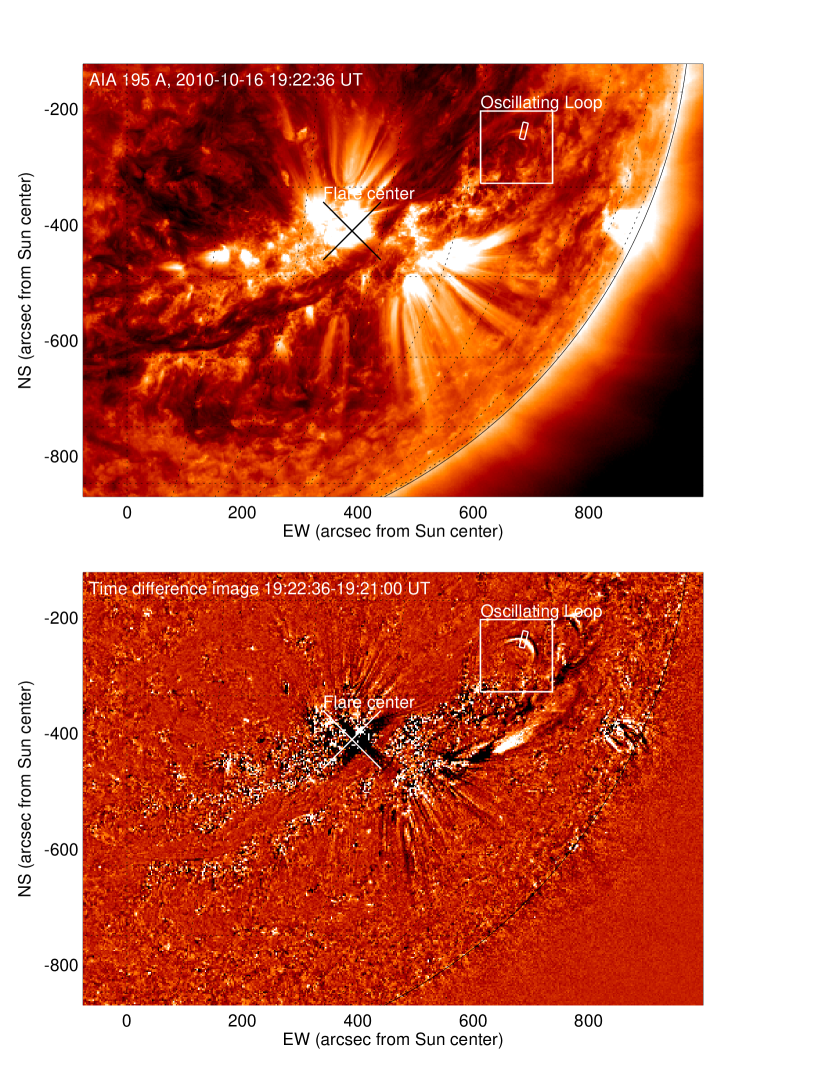
Figure 1: AIA 171 A image of flare observed on 2010-Oct-16 19:22:36 UT shown with the flux on a logarithmic flux scale (top panel) and as difference image with respect to 19:21:00 UT (bottom panel). The flare location is marked with a cross (in the center of the diffraction pattern) and a box indicates the location of the oscillating loop. [See also movies in 171 Å intensity and running-difference format that are available as supplementary data in the electronic version of this journal].

A major flare of GOES class M2.9 occurred on 2010 Oct 16, 19:07-19:12 UT at location W26/S20 ($+390\hbox{${}^{\prime\prime}$}$ west and $-410\hbox{${}^{\prime\prime}$}$ south of Sun center), which triggered a number of loop oscillations in the westward direction of the active region (NOAA 1112). In this study we focus on the detailed analysis of a loop at the loop apex position $+698\hbox{${}^{\prime\prime}$}$ west and $-243\hbox{${}^{\prime\prime}$}$ south of Sun center, which displays prominent oscillations. The location of this loop with respect to the flare center, is shown in Fig. 1. The oscillating loop is discernible as a faint semi-circular structure in the logarithmically-scaled intensity image in 171 Å (Fig. 1, top panel), or even clearer in the difference image (19:22:36 UT - 19:21:00 UT) in Fig. 1 (bottom panel), where the times were chosen at the maximum and subsequent minimum of an oscillation period. The 171 Å intensity image (Fig. 1) shows also irregular moss-like structure in the background of the oscillating loop of similar brightness, which poses some challenge for exact measurements of the loop oscillation parameters, because the background is time-variable, even on the time scale of the oscillation period.

2.3 Transverse Loop Oscillations

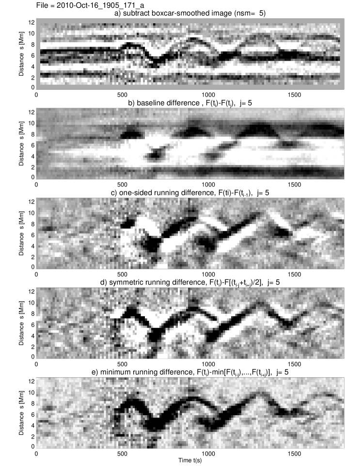
Figure 2: Five different enhancement algorithms to visualize the loop oscillation in a time-slice plot with the time running along the x-axis (time range is 2010-Oct-16 19:05 — 19:35 UT) and the spatial coordinate (defined in Fig. 1 along the stripe perpendicular to the loop through the loop apex): (a) highpass filtering by subtraction of a boxcar-smoothed image (top panel); (b) baseline difference by subtraction of the first time slice (second panel); (c) one-sided running time difference (third panel); (d) symmetric running time difference (fourth panel); and (e) minimum running time difference (bottom panel; $\Delta t=\pm 5$ frames). There appear some “echoes” or “multiple periods”, e.g., around $t\approx 1000$.

Loop oscillations are traditionally investigated most easily in time-difference movies. [Movies of this oscillation event in 171 Å intensity and running-difference format are available as supplementary data in the electronic version of this journal]. However, a variety of time-differencing schemes can be applied in order to enhance the best contrast. We explore a variety of time-differencing schemes in Fig. 2, for a data stripe oriented perpendicular to the loop axis at its apex with a length of 30 pixels and a width of 10 pixels (indicated with a small rectangle in Fig. 1). We construct time-slice plots with $n_{t}=150$ time frames on the x-axis (covering the time interval from 19:05 UT to 19:35 UT with a cadence of $\Delta t=12$ s) and a spatial dimension in direction transverse to the loop on the y-axis (with $n_{y}=30$ pixels), averaged over the $n_{w}=10$ pixels of the stripe width (parallel to the loop). We show 5 different differencing schemes of this time slice in Fig. 2, using a high-pass filter (Fig. 2 top panel), a baseline difference (Fig. 2, second panel), and a one-sided (Fig. 2, third panel), a symmetric (Fig. 2, fourth panel), and a running-minimum difference scheme (Fig. 2, bottom panel), which is defined as

$$\Delta F(t_{i},y_{j})=F(t_{i},y_{j})-min[F(t_{i-k},y_{j}),...,F(t_{i+k},y_{j})],\$$ (1)

so it subtracts a running minimum evaluated within a time interval with a length of $2k$ pixels symmetrically placed around every time slice. Each method has its merits and disadvantages, as it can be seen in Fig. 2. The biggest challenge is the non-uniformity and time variability of the background. An additional complication is the presence of fainter secondary oscillating loops, which appear like “echoes” in the time-slice plots. For further analysis we adopt the running-minimum differencing scheme (Fig. 2, bottom), which appears to have the best signal-to-noise ratio of the oscillating features.

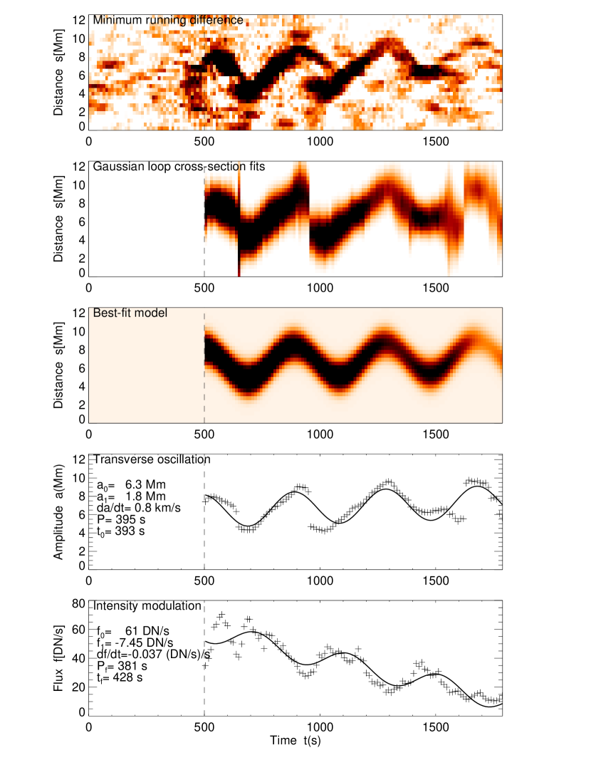
Figure 3: Time-slice diagram of 171 Å flux of oscillating loop with the running-minimum difference method (top panel; $\Delta t=\pm 10$ frames), with Gaussian cross-sectional fits (second panel) and best-fit model (third panel), based on a fit of the transverse oscillation amplitude $a(t)$ with a sine function plus linear motion (fourth panel), and anti-correlated flux modulation $f(t)$ at the oscillating loop apex (bottom panel). The data points are indicated with crosses, while the fit of the theoretical function is outlined with thick solid linestyle. The time axis is given in units of seconds after the start of the time slice at 19:05 UT.

The measurement of the loop oscillation amplitude variation $a(t)$ as a function of time $t$ can be done (i) by localizing the cross-sectional flux maxima in running-difference time-slice plots, (ii) by cross-correlation of subsequent time slices, or (iii) by fitting a Gaussian profile to the cross-sectional flux profiles. We find that the first and the latter method are most robust. From the running-minimum time-slice plot (Fig. 3 top frame) we perform fits of Gaussian profiles $F_{fit}(s,t)$ to the observed cross-sectional flux profiles $F(s,t)$ in each time slice $t$ (using the standard GAUSSFIT.PRO routine in the IDL software),

$$F_{fit}(s,t)=f(t)\exp{\left(-{[s-a(t)]^{2}\over 2\sigma_{s}^{2}(t)}\right)}+b(t)\ ,$$ (2)

which yields the four coefficients of the peak flux $f(t)$, the oscillation amplitude $a(t)$, Gaussian width $\sigma_{s}(t)$, and mean background flux $b(t)$ for each time $t$. The 4-parameter fits The cross-sectional flux profiles $F(s,t)$ and the Gaussian fits $F_{fit}(s,t)$ are shown in Fig. 4 for each time in the interval between $t_{1}$=19:05 UT and $t_{150}$=19:35 UT, while a corresponding time-slice with Gaussian fits is rendered in color scale in Fig. 3 (second panel). The average Gaussian loop width during the oscillation period is $\sigma_{s}=2.1$ Mm, which corresponds to a FWHM loop width of $w=\sigma_{s}2\sqrt{2\ln 2}=4.9\pm 0.6$ Mm.

We are fitting now a sinusoidal function with a linear drift to the location of the oscillation amplitudes $a(t)$ (crosses in Fig. 3, fourth panel), using the Powell optimization routine (Press et al. 1986) from the IDL software,

$$a_{fit}(t)=a_{0}+a_{1}\sin{\left({2\pi(t-t_{0})\over P}\right)}+a_{2}{(t-t_{0})\over P}\ ,$$ (3)

for which we find a midpoint position $a_{0}=6.3$ Mm, a drift velocity $a_{2}/P=0.8$ km/s, an oscillation period of $P=395$ s (6.4 min), an oscillation amplitude $a_{1}=1.8$ Mm, and a sinusoidal onset time of $t_{0}=393$ s after the start of the time slice at 19:05:00 UT, i.e., at 19:11:33 UT. The onset time of the oscillation will be important to measure the exciter speed of the trigger. The fit of the sinusoidal amplitude function $a_{fit}(t)$ to the measured amplitude $a(t)$ is shown in Fig. 3 (fourth panel). The fitted function with a constant amplitude $a_{1}$ appears to be appropriate for the duration of $N_{pulse}=(t_{150}-t_{33})/P=1407/395=3.6$ oscillation periods, since we do not observe any significant damping of the amplitude during this time interval.

2.4 3D Loop Geometry

The projected loop shape is close to a semi-circular geometry (Fig. 1, bottom), and thus we can assume that the loop plane is near the plane-of-sky or nearly perpendicular to the line-of-sight. The location of the loop curvature center is at a distance of $\approx 740\hbox{${}^{\prime\prime}$}$ from Sun center or 0.77 solar radii, which corresponds to a heliographic angle of $\alpha=50^{\circ}$ from disk center.

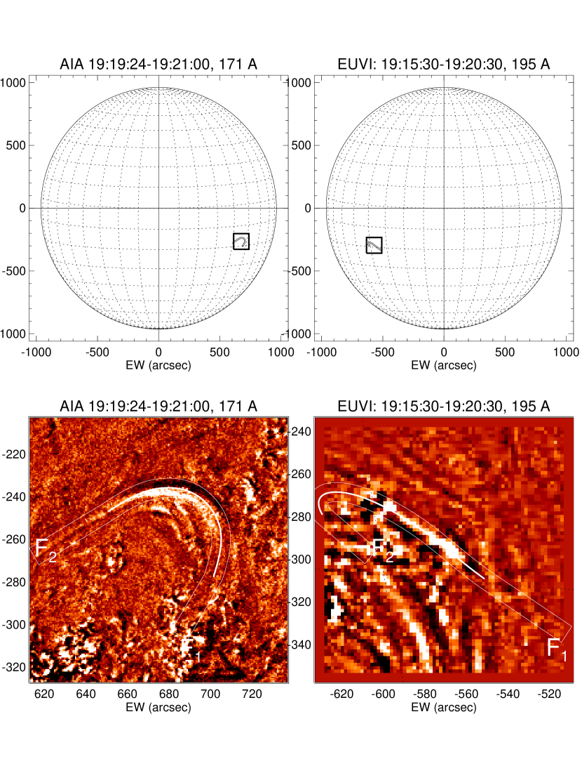
Figure 5: SDO and STEREO observations of oscillating loop: An AIA 171 Å difference image (19:19:24-19:21:00 UT) is shown at the bottom left, and a near-simultaneous STEREO/EUVI/A 195 Å difference image (19:15:30-19:20:30 UT) with additional highpass filtering is shown at the bottom right. The corresponding field-of-views and loop outlines are shown for both instruments in the top panels. The thick solid curve in the AIA image indicates the tracing of the oscillating loop segment, which is fitted to the corresponding loop segment in EUVI/A by 3D coordinate transformations with variable altitudes and inclination angle of the loop plane, which constrains also the extrapolated footpoint locations ($F_{1},F_{2}$) at the solar surface.

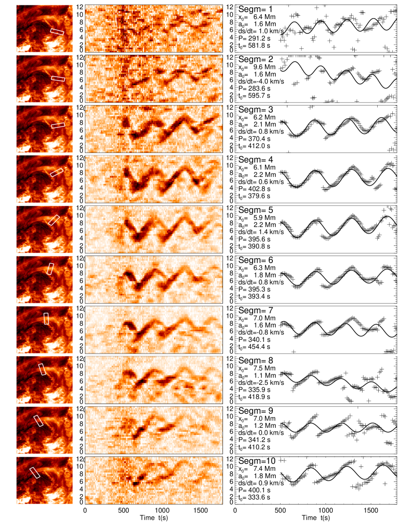
Figure 6: Ten different stripes perpendicular to the loop spine (left panels), used to extract a running-minimum difference plot (middle panels), and sinusoidal fits of the loop oscillation amplitude as a function of the loop position (right panels), from loop segment 1 (near footpoint $F_{1}$) to loop segment 10 (near footpoint $F_{2}$).

The full 3D geometry of the loop can be obtained from the combination of the EUVI instrument onboard STEREO and AIA observations, a procedure that we carry out for the first time here. The loop was in the field-of-view of STEREO/A(head) at this time, but was occulted for STEREO/B. The STEREO/A spacecraft was located on 2010 Oct 16 at a separation angle of $\alpha_{A}=83.583^{\circ}$ to the east of Earth, at a latitude of $\beta_{A}=-0.119^{\circ}$ from the Earth ecliptic plane. In Fig. 5 we show nearly contemporaneous AIA and EUVI/A difference images of the loop, which clearly show the oscillatory motion of the loop, after highpass-filtering of the EUVI/A image. Unfortunately, EUVI/A observed only in a different wavelength of 195 Å at this time, while the oscillation is best visible in the 171 Å channel in AIA. EUVI/A had also a lower cadence ($\approx 5$ min vs. 12 s in AIA) and the spatial resolution of EUVI ($1.6\hbox{${}^{\prime\prime}$}$ pixels) is about three times coarser than AIA ($0.6\hbox{${}^{\prime\prime}$}$ pixels). Nevertheless, the image quality is sufficient to approximately determine the 3D loop geometry. We subtracted the earlier image from the later image, and thus a density increase in the difference images (white in Fig. 5) indicates an inward loop motion (in the AIA image) and a correlated density compression (in the EUVI/A image). We rotate the 2D-coordinates of the loop traced in AIA (Fig. 5 left) into the coordinate system of EUVI/A with variable heights and inclination angle of the loop plane. By matching the position and direction of the loop ridge in EUVI/A we obtain the absolute height range of the traced loop segment, i.e., $21.7<h_{segm}<37.4$ Mm. In order to locate the positions of the footpoints we extrapolate the traced loop segment in both directions and define the positions of the loop footpoints where the coplanar extrapolation intersects with a height $h=0$ above the solar surface. The so-defined extrapolated footpoint positions are found at $F_{1}=(685\hbox{${}^{\prime\prime}$},-305\hbox{${}^{\prime\prime}$})$ (south of traced loop) and $F_{2}=(615\hbox{${}^{\prime\prime}$},-268\hbox{${}^{\prime\prime}$})$ (east of trace loop) with respect to Sun center (Fig. 5). The apex or midpoint of the traced loop segment (at $s=L_{loop}/2$) is located at position $(x_{apex},y_{apex})=(698\hbox{${}^{\prime\prime}$},-243\hbox{${}^{\prime\prime}$})$, for which we show time-slice plots of the oscillation in Figs. 2-4 (i.e., segment #6 in Fig. 6). The apex location will also be used to define the arrival time of the exciting wave and starting time of the loop oscillation in Section 2.11. The inclination angle of the loop plane to the local vertical is found to be $\vartheta\approx 20^{\circ}\pm 20^{\circ}$, but cannot be determined more accurately because of the short loop segment detectable in EUVI/A.

From the absolute 3D coordinates $(x_{i},y_{i},z_{i}),i=1,...,n$ of the stereoscopically triangulated loop we can calculate the full loop length $L_{loop}$,

$$L_{loop}=\sum_{i=0}^{n-1}\sqrt{\left[(x_{i+1}-x_{i})^{2}+(y_{i+1}-y_{i})^{2}+(z_{i+1}-z_{i})^{2}\right]}\ ,$$ (4)

for which we find $L_{loop}=163$ Mm. The traced loop segment over which amplitude oscillations are clearly visible covers the fraction from $s_{1}/L=0.23$ to $s_{2}/L=0.78$ of the total loop length and has only a length of $L_{segm}=123$ Mm. If we approximate the 3D loop geometry with a coplanar semi-circular shape, the loop curvature radius is estimated to be $r_{loop}\approx L_{loop}/\pi=52$ Mm.

The plane of transverse loop oscillations with respect to the average loop plane cannot accurately be determined with the existing STEREO data, but they are roughly coplanar, based on the centroid motion constrained by AIA that is absent in EUVI/A from a near-perpendicular view (Fig. 5). Coplanar kink mode oscillations corresponds to a vertical polarization.

2.5 Spatial Variation of Loop Oscillation

In a next step we analyze the spatial variation of the transverse kink-mode oscillation $a(t)$ as a function of the spatial loop position, which we specify with a segment number running from segment #1 at the loop length coordinate $s_{1}/L=0.23$ (near the first footpoint $F_{1}$) to segment #10 at $s_{2}/L=0.78$ (near the second loop footpoint). This analysis serves a two-fold purpose: (1) to detect possible asymmetries of the kink mode, and (2) to detect possible propagating waves.

In Fig. 6 we show the analysis of the loop oscillation of 10 different loop segments, numbered consecutively (# 1-10) from the southern loop footpoint $F_{1}$ to the north-eastern footpoint $F_{2}$ along the loop axis with loop length coordinate $s$. The location and orientation of the time-slice stripes is indicated in the left panels of Fig. 6, the running-minimum difference time slices are shown in the middle panels of Fig. 6, and the sinusoidal fits $a_{fit}(t)$ to the loop amplitudes in the right-hand panels of Fig. 6, which also contains the best-fit parameters. If we discard the the two noisiest segments near footpoint $F_{1}$ (Segment #1 and #2 in Fig. 6), we obtain for the others a mean amplitude of $\langle a_{1}(s)\rangle=1.8\pm 0.4$ Mm, a mean period of $\langle P(s)\rangle=373\pm 30$ s (6.2$\pm$0.5 min), and a mean starting time of $\langle t_{0}(s)\rangle=399\pm 35$ s. Thus the variation of best-fit periods and starting times is only $\approx 8\%$, and thus we conclude that there is no significant phase shift of the oscillation amplitude along the loop that could be considered as a propagating wave. Thus, we deal with a pure standing wave of the fast MHD kink-mode.

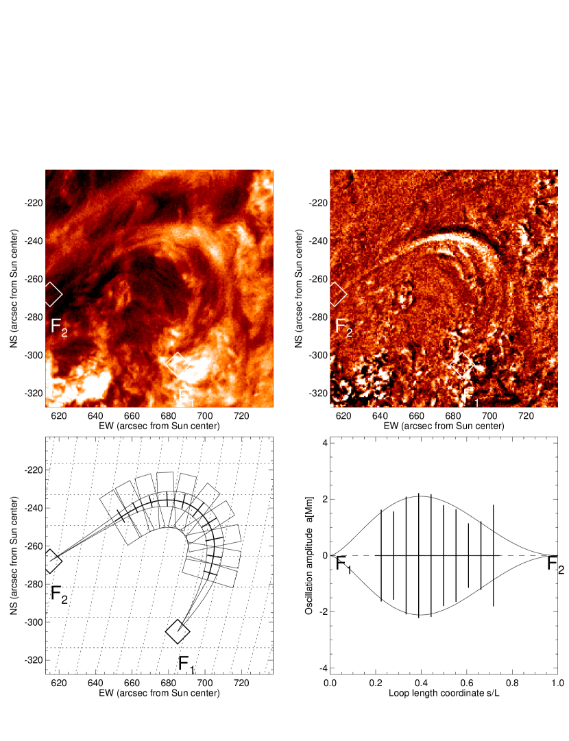
Figure 7: Location of stereoscopically triangulated loop footpoints (marked with diamonds and labeled with $F_{1}$ and $F_{2}$) and 10 loop segments with the rectangular subimages over which the 10 time slices (shown in Fig. 6) were extracted (bottom left panel). The corresponding AIA 171 Å image (top left) and difference image 19:21:00-19:19:24 UT (top right) are also shown. The magnitude of the transverse kink-mode oscillation amplitude is indicated with thick bars (bottom panels), which fit a stretched sine function (Eq. 5).

In Fig. 7 we show the spatial variation of the oscillation amplitude $a_{1}(s)$ in the context of an intensity image (Fig. 7, top left) and a running-minimum difference image (Fig. 7, top right). The locations of the 10 azimuthal time-slice stripes are shown in Fig. 7 (bottom left), over which the amplitude oscillation were measured in Fig. 6. The dependence of the oscillation amplitude $a_{1}(s)$ along the loop shows a maximum amplitude of $a_{1}^{max}=2.0$ Mm near the loop apex. A sinusoidal displacement along the loop axis is ideally expected for a kink eigen-mode with fixed nodes (compare with the analogy of a violin string). Our measurements, however, rather show a slightly distorted and asymmetric function, which can be approximated by a squared sine function (to account for the curvature of the loop) and a nonlinear dependence $a(s^{0.75})$ on the loop length (to account for the asymmetry of the loop, as evident from the stereoscopic triangulation of the footpoints, see Fig. 7 bottom right panel),

$$a_{1}(s)=a_{1}^{max}\sin^{2}{\left[\pi\left({s\over L}\right)^{0.75}\right]}\ ,$$ (5)

where $s=0$ and $s=L$ mark the nodes at the true footpoints $F_{1}$ and $F_{2}$. The observed oscillation amplitudes $a(s)$ follow the squared sine function closely in the range of $s/L\lower 1.72218pt\hbox{$\;\buildrel<\over{\scriptstyle\sim}\;$}0.6$, but deviate in the range of $0.6\lower 1.72218pt\hbox{$\;\buildrel<\over{\scriptstyle\sim}\;$}s/L\lower 1.72218pt\hbox{$\;\buildrel<\over{\scriptstyle\sim}\;$}0.75$, probably because of the interference of a secondary oscillating loop.

2.6 Multiple-Loop Oscillations

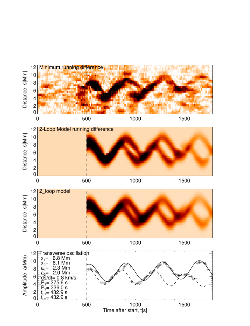
Figure 8: Two-loop oscillation model fitted to the same oscillation amplitudes $a(t)$ as measured in Segment #6 shown in Figs. 3 and 4. The amplitudes of the two oscillating loops are indicated with solid and dashed curves (bottom panel). The two-loop solution is also visualized as time-slice plots for the absolute flux (third panel) and running-minimum difference representation (second panel).

From watching the AIA 171 Å movies (see electronic supplementary data to this paper) and from the time-slice plots shown in Figs. 2, 3, and 6 it appears that multiple loops are involved in kink-mode oscillations. The previous analysis has determined the average dynamic parameters of the collective ensemble of individual loop strands. In Figure 8 we are fitting a 2-loop model to the time-slice plots obtained near the loop apex, which yields slightly different periods ($P_{1}=375$ s and $P_{2}=336$ s), oscillation amplitudes ($a_{1}=2.3$ Mm and $a_{2}=2.0$ Mm), and loop centroid positions ($x_{1}=6.8$ Mm and $x_{2}=6.1$ Mm), but a common start time $t_{0}=423$ s (i.e., 19:12:03 UT). Thus the loops are excited in phase, but the secondary loop has an oscillation period that is about 10% shorter. The secondary loop seems also to have a shorter lifetime and is only visible in the 171 Å filter for about 2 oscillation periods (compared with 3.6 periods of the primary loop.)

2.7 Intensity Modulation During Loop Oscillations

The 171 Å intensity of the background-subtracted loop intensity exhibits strong modulations, being strongest near the beginning, but fading out gradually at the end of the time interval of oscillations. We show in Fig. 3 (bottom panel) the background-subtracted intensity flux profile $f(t)$ as measured near the loop apex from the Gaussian cross-sectional profile fits (Eq. 2). Amazingly, the intensity flux modulation appears to be in synchronization with the oscillation amplitude, which is a very interesting property that we have not noticed in previous observations of loop oscillations (e.g., in the 26 cases observed with TRACE; Aschwanden et al. 1999, 2002). In fact, the loop flux modulation $f(t)$ (Fig. 3, bottom panel) occurs in anti-phase to the amplitude modulation $a(t)$ that is measured in upward direction away from the loop curvature center. In addition to the oscillation-modulated variation, the flux decays as a function of time, which can be described with a linear decay rate $df/dt$, similar as found for 8 loops with kink-mode oscillations during the 2001 Apr 15, 21:58 UT, flare (Aschwanden and Terradas 2008). Thus, we fit a sinusoidal function with a linear decay rate $f_{2}/P_{f}$,

$$f_{fit}(t)=f_{0}+f_{1}\sin{\left({2\pi(t-t_{f})\over P_{f}}\right)}+f_{2}{(t-t_{f})\over P_{f}}\ .$$ (6)

We find a peak flux of $f_{0}=61$ DN s^-1, a flux modulation of $f_{1}=7.5$ DN/s, a linear decay rate of $f_{2}/P_{f}=-0.037$ (DN s^-2), which defines a loop lifetime of $t_{life}=P_{f}(f_{0}/f_{2})=1649$ s (27 min) and is compatible to the loop cooling times $\tau_{cool}=17\pm 7$ min found in Aschwanden and Terradas (2008), modeled also in Morton and Erdelyi (2009, 2010). It is therefore suggestive to interpret the observed lifetime of the oscillating loop as the detection time of a loop that cools through the AIA 171 Å passband. For the flux modulation that is anti-correlated with the amplitude oscillation we suggest an interpretation in terms of density compression by cross-sectional loop width oscillations, similar to a sausage mode, which is modeled in the next section.

2.8 Density Modulation During Loop Oscillations

In the previous Sections we established that the vertical oscillation amplitude amounts to $a_{1}^{max}/r_{loop}=2/52=4\%$. If we assume that the loop is embedded in a magnetic field with a constant pressure across the loop cross-section (to first order) in a low plasma $\beta$-parameter environment, the ambient magnetic field lines are expected to oscillate in synchronization with a displacement that is proportional to the loop amplitude. A consequence of this scenario is that the loop cross-sectional radius $r(t)-r0$ varies proportionally to the loop amplitude $a(t)$,

$$r(t)=r_{0}\left(1+{a(t)\over r_{loop}}\right)\ ,$$ (7)

leading to a modulation of the loop cross-sectional area $A(t)=\pi r^{2}(t)$ that scales quadratically to the loop radius $r(t)$,

$$A(t)=A_{0}\left(1+{a(t)\over r_{loop}}\right)^{2}\ .$$ (8)

Since the loop footpoints are anchored at fixed positions in the photosphere, we can characterize the oscillating loop shape with an elliptical geometry to first order, which oscillates around the semi-circular geometry of the loop at rest, as depicted in Fig. 7. The loop length of a half ellipse is mathematically (to first order),

$$L=\pi{r_{minor}+r_{major}\over 2}+...\ ,$$ (9)

where $r_{minor}$ is the minor semi-axis and $r_{major}$ is the major semi-axis of the ellipse. For the semi-circular limit the radii are equal, $r_{minor}=r_{major}=r_{loop}$, and the half loop length is $L=\pi r_{loop}$. Assigning the minor axis to the half footpoint separation, $r_{minor}=r_{loop}$, and the major axis to the vertical radius with a small oscillation amplitude, $r_{major}=r_{loop}+a(t)$, the elliptical loop length varies (to first order) as,

$$L(t)=\pi\left(r_{loop}+{a(t)\over 2}+...\right)=\pi r_{loop}\left(1+{a(t)\over 2r_{loop}}+...\right)\ .$$ (10)

The volume of the loop, $V(t)$, varies then consequently with the 5/2-power of the amplitude variation (to first order),

$$V(t)=A(t)L(t)=V_{0}\left(1+{a(t)\over r_{loop}}+...\right)^{5/2}\ .$$ (11)

The electron density inside the loop, assuming particle conservation in adiabatic compression and expansion processes, varies then reciprocally to the loop volume,

$$n_{e}(t)\propto V(t)^{-1}=n_{0}\left(1+{a(t)\over r_{loop}}+...\right)^{-5/2}\ .$$ (12)

For optically thin emission, as it is the case in EUV and soft X-rays for coronal conditions, the flux intensity scales with the square of the electron density times the column depth $dz$ (which is here assumed to be proportional to the loop diameter $dz\propto\sqrt{A(t)}$), yielding an anti-correlation of the flux with the 4-th power of the amplitude oscillation,

$$F(t)\propto n_{e}^{2}(t)\ dz(t)=F_{0}\left(1+{a(t)\over r_{loop}}+...\right)^{-4}\ .$$ (13)

Thus, the small-amplitude variation of $a_{1}^{max}/r_{loop}=2.2/52=0.042$ is amplified with the 4-th power,

$$F_{max}=F_{0}\left(1-4{a_{1}^{max}\over r_{loop}}+...\right)\approx 1.18^{-1}\ ,$$ (14)

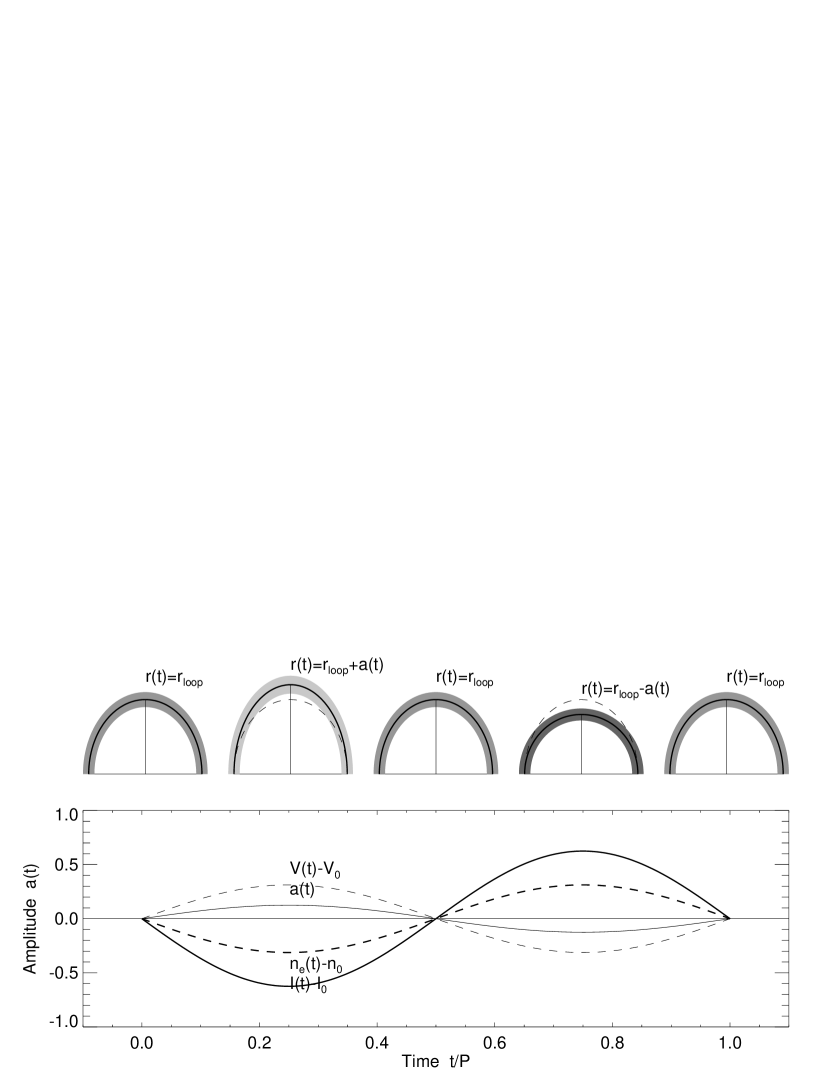
Figure 9: Schematic of sinusoidal modulation of the loop vertical radius $r(t)=r_{loop}+a(t)$, volume $V(t)-V_{0}$, density $n_{e}(t)-n_{0}$, and flux intensity $I(t)-I_{0}$ during one full oscillation period. Note that the density and intensity vary in anti-correlation to the loop amplitude, indicated with the grey-scale shading of the loops.

which yields a flux modulation of 18% with respect to the mean value $f_{0}$. In Fig. 3 (bottom panel) we fitted the flux variation and found indeed an average mean modulation factor of $q_{f}=f_{1}/\langle f_{0}(t)\rangle\approx 7.45/30)\approx 24\%$, for the average of the total flux $\langle f_{0}(t)\rangle\approx(61+10)/2\approx 30$ DN s^-1 during the oscillatory episode. Thus our model predicts the correct time phase and approximate amount of oscillatory intensity flux modulation, which is anti-correlated to the sinusoidal loop amplitude oscillation (Fig. 9). The MHD wave mode that is associated with cross-sectional variation is called sausage mode or symmetric $m=0$ mode of fast MHD waves (e.g., Roberts 1984), which has a distinctly different eigen-mode period than the kink mode. The cross-sectional and density variation that were found in synchronization with the kink mode here (which has the same geometric and density properties as the sausage mode, but a different period than predicted by the MHD dispersion relation), is a novel result of this study. This characteristic seems to be a particular property of oscillations in the loop plane (Fig. 7), also called “vertical polarization of kink mode” (Wang and Solanki 2004; Verwichte et al. 2006a,b), which would not occur (to first order) for transverse oscillations in perpendicular direction to the loop plane.

2.9 Density and Temperature Analysis of Oscillating Loop

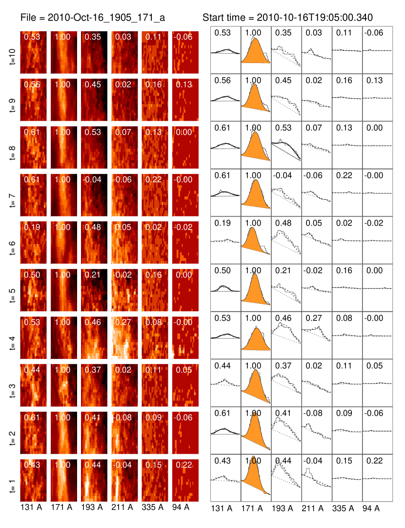
Figure 10: Cross-sectional loop profiles in 6 AIA filters and at 10 different times during the oscillation episode from 19:05 to 19:35 UT. The wavelength of the primary loop detection is 171 Å, with which the subimages are cross-scorrelated (with the cross-correlation coefficients given in each panel).

Having the 6 coronal AIA filters available that cover a temperature range of $T\approx 0.6-16$ MK for the entire oscillation episode with the same cadence of 12 s we are in an unprecedented position to conduct an accurate diagnostics of the electron temperature and density of the oscillating loop. For this purpose we extract loop-aligned subimages in all 6 coronal wavelengths in 10 spatial segments ($s_{i},i=1,...,10$) at the loop locations as indicated in Fig. 7 (bottom left) and at 10 consecutive times ($t_{j},j=1,...,10$) during the time interval of 19:05-19:35 UT. We show the $6\times 10$ subimages for the 10 different times for loop segment # 6 near the loop apex in Fig. 10 (left half), as well as the averaged cross-sectional loop profiles resulting from these subimages in Fig. 10 (right half). We calculate also the cross-correlation coefficients of these subimages with the simultaneous subimage in the detected wavelength of 171 Å (indicated by the numbers in each subpanel in Fig. 10). From this information shown in Fig. 10 it is very clear that the oscillating loop exhibits a near-Gaussian cross-sectional profile only in the 171 Å filter, while the 131 and 193 Å filters show only a mild correlation ($CCC\approx 0.4-0.5$) and the remaining filters (211, 335, and 94 Å) are absolutely uncorrelated ($CCC\approx 0.0-0.1$), which already narrows down the loop temperature to peak response temperature of the 171 Å filter at $T\approx 10^{5.9}\approx 0.8$ MK.

In Fig. 11 (left side) we show the AIA temperature response functions, where the low-temperature response of the 94 A filter is corrected by an empirical factor of $q_{94}=6.7\pm 1.7$ (Aschwanden and Boerner 2011). The total fluxes $f^{tot}(t)$ (histograms with error bars in Fig. 11 middle panels) and background fluxes $f^{back}(t)$ (hatched areas in Fig. 11 middle panels) are also shown, where the background is evaluated based on the Gaussian cross-sectional fits (Fig. 10). The difference $f^{loop}(t)=f^{tot}(t)-f^{back}(t)$ is attributed to the EUV flux of the oscillating loops and is modeled with a single-Gaussian differential emission measure (DEM) distribution by forward-fitting (according to the method described in Aschwanden and Boerner 2011),

$$EM(T)=EM_{0}\ \exp{\left(-{(T-T_{0})^{2}\over 2\sigma_{T}^{2}}\right)}\ ,$$ (15)

with the best-fit DEM solutions shown in Fig. 11 (top right panel) for the 10 consecutive time steps. The single-Gaussian DEM fits yield an average peak temperature of $T_{0}=0.57\pm 0.14$ MK and a Gaussian temperature width of $\sigma_{log(T)}=0.18\pm 0.10$ (Fig. 11, right side), which corresponds to a near-isothermal temperature distribution at the limit of the temperature resolution $\Delta log(T)\approx 0.3$ of the AIA filters, similarly as found for a statistical set of other loops analyzed from TRACE (Aschwanden and Nightingale 2005) or AIA (Aschwanden and Boerner 2011). The goodness-of-fit of the best-fit DEM solutions is found to be $\chi^{2}_{red}=1.10\pm 0.05$. The average agreement of the observed and modeled fluxes is found to be $\lower 1.72218pt\hbox{$\;\buildrel<\over{\scriptstyle\sim}\;$}3\%$ in the three filters with the highest fluxes (Fig. 11, middle column). The largest relative deviation occurs in the 94 Å filter, which are known to have an incomplete temperature response function due to missing lines of Fe X transition (Aschwanden and Boerner 2011). Also we have to keep in mind that the largest flux deviations in the fits are only in the order of $\approx 0.2-0.5$ DN/s in the 94, 131, and 335 Å channels, which results mostly from uncertainties in the (time-variable) background evaluation rather than from the statistical photon noise.

Assuming a filling factor of unity, we can estimate the mean electron density in the oscillating loop,

$$n_{0}=\sqrt{EM_{0}\over w}\ ,$$ (16)

for which we obtain a mean value of $n_{0}=(1.9\pm 0.3)\times 10^{8}$ cm^-3, based on average loop widths of $w=4.9\pm 0.6$ Mm (Fig. 11, right side), which is measured near the apex of the loop for the segment # 6 shown as cross-sectional loop profiles in Fig. 10.

2.10 Radiative Cooling Time Scale

Since the issue has been raised that the lifetime of oscillating loops (defined by the detection time in a given temperature filter) is commensurable with the duration of an observed oscillation event (Aschwanden and Terradas 2008; Morton and Erdelyi 2009), let us explore whether the theoretically predicted time scales are consistent with the observed flux decay. At the relatively low coronal temperatures of $T_{e}\lower 1.72218pt\hbox{$\;\buildrel<\over{\scriptstyle\sim}\;$}1.0$ MK observed in EUV, radiative cooling is the dominant time scale, while conductive cooling is only relevant at much hotter plasma temperatures in soft X-rays. Assuming an impulsive heating episode with subsequent cooling we can approximate the temperature evolution with an exponentially decaying function over some temperature range,

$$T_{e}(t-t_{1})=T_{e}(t_{1})\ \ \exp{\left[-{(t-t_{1})\over\tau_{cool}}\right]}\ ,$$ (17)

where the temperature cooling time $\tau_{cool}$ corresponds to the radiative cooling time $\tau_{rad}$,

$$\tau_{rad}(n_{0},T_{0})={9\over 5}{k_{B}T_{0}^{5/3}\over n_{0}\Lambda_{0}}\ ,$$ (18)

with $\Lambda_{0}\approx 10^{-17.73}$ erg cm³ s^-1 being the radiative loss rate at EUV temperatures ($T\approx 1.0$ MK). For our measured values of $T_{0}=0.57$ MK and $n_{0}=1.9\times 10^{8}$ cm^-3 at the loop apex we estimate $\tau_{rad}\approx 2750$ s (46 min). The loop lifetime $\tau_{171}$ in the 171 Å filter, which has a FWHM temperature range of $T_{171}=0.53-1.17$ MK, is then $\tau_{171}=2200$ s (37 min) according to Eq. 17, which if fully consistent with the observed flux decay time $\tau_{life}=P_{f}(f_{0}/f_{2})=1650$ s (27 min) based on the fitted time profile (Eq. 6) to the measurement shown in Fig. 3 (bottom panel). Therefore, we can interpret the observed flux decay seen in the 171 Å as a consequence of the radiative cooling time. Based on this cooling scenario we would predict an initial temperature of $T_{e}(t=t_{1})\approx 0.8$ MK at the beginning of the oscillation event and a temperature of $T_{e}(t=t_{2})\approx 0.4$ MK at the end of the oscillation episode. The predicted temperature drop $T_{e}(t)$ for a single loop cannot be retrieved by the DEM modeling (Fig. 11, left second panel), because the two nearly cospatial oscillating loops cannot be separated and thus we can only measure the combined emission measure-weighted temperature evolution of near-cospatial loops. Considering the analysis of the temperature evolution in other channels, only the 131 Å channel has a temperature response to slightly lower values than the 171 Å channel, but is about two orders of magnitude less sensitive and thus is unsuitable for a quantitative analysis.

2.11 Excitation of Loop Oscillations

The exciter or trigger of the loop oscillations is very likely the associated flare event to the east of the oscillating loop. If we calculate the projected distance between the flare site $(x_{flare}=+390\hbox{${}^{\prime\prime}$},y_{flare}=-410\hbox{${}^{\prime\prime}$})$ (section 2.2) and the apex of the oscillating loop $(x_{apex}=+698\hbox{${}^{\prime\prime}$},y_{apex}=-243\hbox{${}^{\prime\prime}$},h_{apex}\approx 50\hbox{${}^{\prime\prime}$})$ (section 2.4), taking the stereoscopically triangulated 3D loop position into account, we obtain and Euclidian distance of $L_{exc}=353\hbox{${}^{\prime\prime}$}$ (256 Mm). Given the time delay between the start of the loop oscillation at the apex (19:12:12 UT) and the flare start (19:10:00 UT; $\pm 6$ s), we obtain the following 3D propagation speed of the exciter,

$$v_{exc}={L_{exc}\over T_{exc}}={256,000\ {\rm km}\over 132\pm 6{\ \rm s}}=1940\pm 125\ {\rm km\ s}^{-1}\ ,$$ (19)

which is a typical Alfvénic (magneto-acoustic) speed in the solar corona. Thus, we can conclude that the loop oscillation is initially triggered by a fast MHD wave with Alfvénic speed. Moreover, the direction of the initial excitation in west-ward direction is in the same direction as the propagation direction of the fast MHD wave that propagates with Alfvénic speed concentrically away from the flare site. Although the angle between the Alfvénic wave direction and the loop oscillation amplitude cannot be determined with high accuracy, it is closer to parallel than perpendicular, as would be expected in a vortex-shedding scenario (Nakariakov et al. 2009), where the kink-mode oscillation occurs in perpendicular direction to the local plasma flow direction. In the case analyzed here, it appears that the plasma volume in the westward direction is stretched out in the same direction, probably following a narrow-angle cone of open magnetic field where the CME escapes. An associated CME on the south-west side of the Sun is visible in SOHO/LASCO and EIT movies. Generally, excitation of kink-mode oscillations with vertical polarization are rare, because they need special circumstances with an exciter near the curvature center of the loop (Selwa et al. 2011).

2.12 External/Internal Density Ratio of Oscillating Loop

Coronal seismology allows us to determine the mean magnetic field in a loop in the kink-mode oscillation mode based on the internal Alfvén speed $v_{A}$ inside the oscillating loop,

$$v_{A}={B_{i}\over\sqrt{4\pi\rho_{i}}}\ .$$ (20)

which can be related to the (fundamental) kink-mode period $P_{kink}$ using the phase speed $c_{k}$ inside the flux tube (Roberts et al. 1984),

$$P_{kink}={2L_{osc}\over c_{k}}={2L_{osc}\over v_{A}}\sqrt{{1+\rho_{e}/\rho_{i}}\over 2}\ ,$$ (21)

which depends on the total length $L_{osc}$ of the oscillating loop and the densities externally ($n_{e}$) and internally ($n_{i}$) of the loop.

On the other hand, we can estimate the external Alfvén speed $v_{Ae}$, which depends on the external magnetic field $B_{e}$ and density $n_{e}$,

$$v_{Ae}={B_{e}\over\sqrt{4\pi\rho_{e}}}\ .$$ (22)

If we interpret the exciter speed $v_{exc}$ between the flare site and the (apex) location of the oscillating loop (Eq. 19) as an Alfvénic wave, we obtain a direct measurement of the external Alfvén speed (supposed the wave is not super-Alfvénic),

$$v_{Ae}=v_{exc}={L_{exc}\over T_{exc}}\ .$$ (23)

Moreover, since the magnetic pressure is generally dominant over thermal pressure in the solar corona, the magnetic field $B_{i}$ internally and $B_{e}$ externally to the loop boundary have to match for a self-consistent magnetic field model of a loop embedded into an external plasma. Based on the definitions of the Alfvén speeds (Eqs. 20, 22), the ratio of the Alfvén speeds depends then only on the density ratio,

$$B_{e}=B_{i}\mapsto{v_{Ae}\over v_{A}}=\sqrt{n_{i}\over n_{e}}\ ,$$ (24)

which can be directly determined from the kink-mode period, loop length, and exciter speed with Eqs. (21) and (23),

$${n_{i}\over n_{e}}={1\over 2}\left({L_{exc}\over L_{osc}}{P_{kink}\over T_{exc}}\right)^{2}-1\ .$$ (25)

Some uncertainty arises from the unknown positions of the actual nodes of the kink mode. Since the oscillation has only been observed over a loop segment of $L_{seg}=123$ Mm, which is a lower limit of the node separation, while the stereoscopically triangulated full loop length $L_{loop}$ down to the solar surface represent an upper limit, we might estimate a realistic value with uncertainty from the arithmetic mean of the two limits, i.e., $L_{osc}\approx(L_{loop}+L_{seg})/2=143\pm 20$ Mm. Thus, for the physical parameters determined above ($L_{exc}=256$ Mm, $T_{exc}=132\pm 10$ s), and the best-fit values of the primary oscillating loop (Fig. 8: $L_{osc}\lower 1.72218pt\hbox{$\;\buildrel<\over{\scriptstyle\sim}\;$}(L_{loop}+L_{seg})/2=143\pm 20$ Mm, $P_{kink}=375.6$ s), we obtain a value of ${n_{i}/n_{e}}\approx 12.0\pm 1.8$, or an inverse ratio of ${n_{e}/n_{i}}\approx 0.08\pm 0.01$. This value is commensurable with alternative methods, using stratified hydrostatic density models of the background corona, for which a statistical average of ${n_{e}/n_{i}}=0.30\pm 0.16$ was found. (Aschwanden et al. 2003). Consequently, for a density ratio of $n_{e}/n_{i}\approx 1/12$, the ratio of the Alfvén speeds is then expected to be $(v_{Ae}/v_{A})=\sqrt{n_{i}/n_{e}}\approx\sqrt{12}\approx 3.4$. In our case, the external Alfvén speed is $v_{Ae}\approx 1940\pm 100$ km s^-1, and the internal Alfvén speed is $v_{A}\approx 560\pm 100$ km s^-1.

2.13 Magnetic Field Modeling

With this novel method of measuring the density ratio ${n_{e}/n_{i}}$ from Alfvénic propagation speeds external and internal to the fluxtube, the magnetic field in the oscillating flux tube and immediate surroundings is then fully constrained with Eqs. 20 and 21 (Nakariakov et al. 1999),

$$B={L_{osc}\over P_{kink}}\sqrt{8\pi\mu m_{p}n_{i}(1+n_{e}/n_{i})}\ ,$$ (26)

for which we obtain $B=4.0\pm 0.7$ G, based on the measurements of $L_{osc}=(143\pm 20)\times 10^{8}$ cm, $P_{kink}=375.6$ s, $n_{i}=(1.9\pm 0.3)\times 10^{8}$ cm^-3, and the density ratio $(n_{e}/n_{i})\approx 0.08\pm 0.01$.

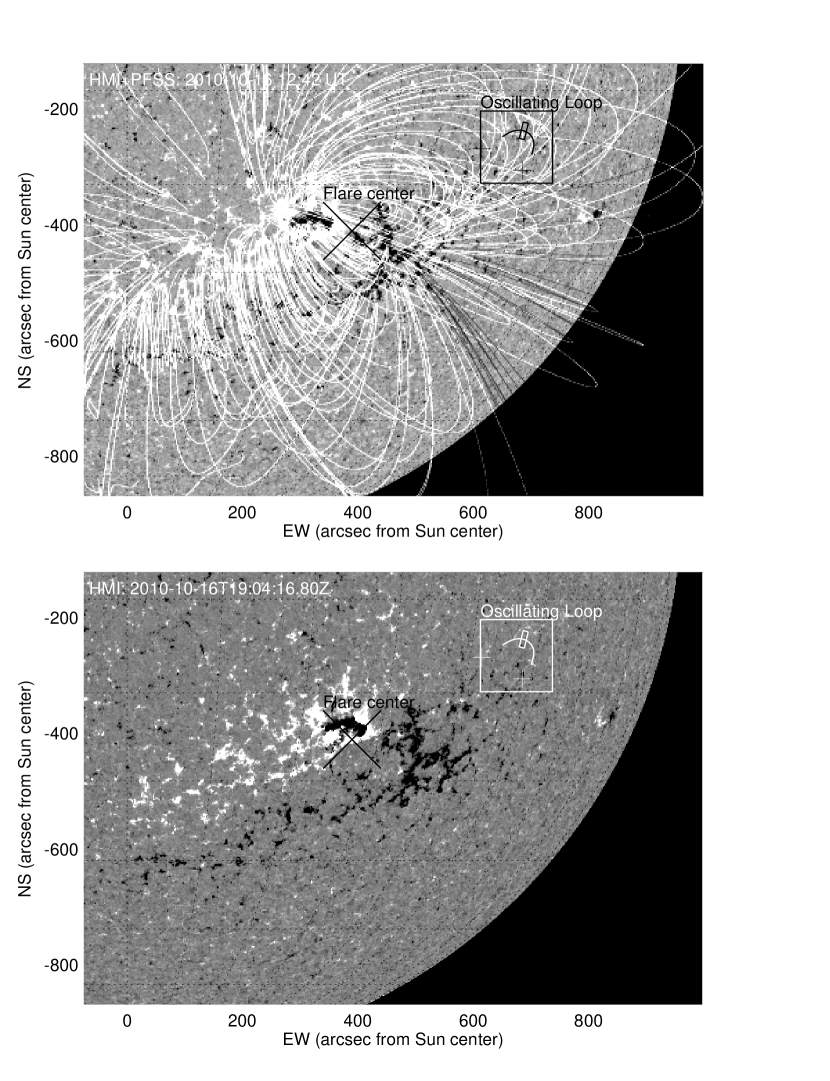
Figure 12: HMI magnetogram of same field-of-view as shown in Fig. 1, with potential field source surface (PFSS) model field lines (top) and locations of flare (diagonal cross), oscillating loop segment (curve), and stereoscopically triangulated footpoints (crosses) indicated.

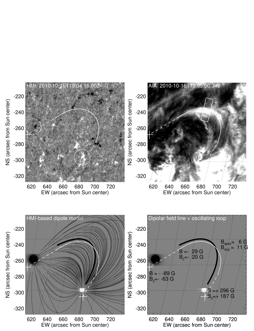
Figure 13: Enlarged field-of-view (identical to Figs. 5 and 7) of the HMI magnetogram (top left), AIA 171 Å image (top right), and HMI-based dipolar potential field model (bottom right) of oscillating loop (white curves). A field line that closely coincides with the oscillating loop is shown separately (bottom right; black curves), constrained by the longitudinal magnetic field observed in the HMI magnetograms with $B_{\parallel 1}=187$ G and $B_{\parallel 2}=-63$ G.

This magnetic field scenario can be tested with observed magnetic field data from the Helioseismic and Magnetic Imager (HMI) on SDO. In Fig. 12 (bottom) we show a HMI magnetogram recorded at 19:04:16 UT, at the beginning of the analyzed time interval. The flare location is situated in the core of the AR, right at the neutral line with the largest magnetic flux gradient, while the oscillating loop is located beyond the western boundary of the active region in a low magnetic-field region that is governed by a “salt-and-pepper pattern” of positive and negative magnetic pores (see enlargement in Fig. 13 top left). A potential-field source surface (PFSS) model calculation is shown in Fig. 12 (top panel), which is dominated by a bipolar arcade above the neutral line in east-west direction.

The magnetic field in the environment of the oscillating loop can be modeled with potential-field or non-potential field models, but both are known to show misalignments with the 3D geometry of stereoscopically triangulated loops of the order of $\alpha_{mis}\approx 20^{\circ}-40^{\circ}$ (DeRosa et al. 2009; Sandman et al. 2009), while simple potential field models calculated from a small set of unipolar magnetic charges (Aschwanden and Sandman 2010) or magnetic dipoles (Sandman and Aschwanden 2010) achieved a reduced misalignment of $\alpha_{mis}=13^{\circ}-20^{\circ}$. For a simple plausibility test of the magnetic field strength inferred from coronal seismology, we model the 3D field at the location of the oscillating loop with an analytical model of two unipolar charges with opposite magnetic polarities that are buried in depths $z_{1}$ and $z_{2}$ and have maximum longitudinal magnetic field strengths of $B_{\parallel 1}=+187$ G and $B_{\parallel 2}=-63$ G at the observed positions $(x_{1},y_{1})$ and $(x_{2},y_{2})$ of the nearest magnetic pores in the HMI magnetogram (marked with circles in Fig. 13, top left panel), where $(x,y,z)$ is a cartesian coordinate system with the xy-plane parallel to the solar surface. The corresponding absolute field strengths vertically above the buried charges are $B_{1}=B_{\parallel 1}/\cos(\vartheta_{1})=296$ G and $B_{2}=B_{\parallel 2}/\cos(\vartheta_{2})=-89$ G, where $\vartheta_{j}$ are the line-of-sight angles. Thus, in this model we have only the two free variables of the depths $z_{1}$ and $z_{2}$ to fit the model of resulting magnetic field lines to the observed loop. The magnetic field resulting from the superposition of two unipolar magnetic charges is then given by (Aschwanden and Sandman 2010),

$${\bf B}({\bf x})=\sum_{j=1}^{N}{\bf B}_{j}({\bf x})=\sum_{j=1}^{N}B_{j}\left({z_{j}\over r_{j}}\right)^{2}{{\bf r}_{j}\over r_{j}}\ ,$$ (27)

in terms of the vector ${\bf r}_{j}=[(x-x_{j}),(y-y_{j}),(z-z_{j})]$, with ${\bf x}_{j}=(x_{j},y_{j},z_{j})$ being the locations of the buried unipolar magnetic charges and $B_{j}$ the magnetic field strength at the solar surface above the magnetic charges. The ratio of the two free variables $z_{1}$ and $z_{2}$ determine the asymmetry of the field lines. For the observed oscillating loop we find values of $z_{1}=0.5\hbox{${}^{\prime\prime}$}$ and $z_{2}=1.5\hbox{${}^{\prime\prime}$}$ to reproduce approximately the observed shape (Fig. 13, bottom left). The field line that closest fits the projected location of the oscillating loops has magnetic field strenghts of $B_{1}=296$ G and $B_{2}=29$ G at the photospheric field line footpoints and $B=6$ G at the apex, which compares favorably with the magnetic field strength of $B_{kink}=4.0\pm 0.7$ G deduced from coronal seismology.

However, since the magnetic field $B(s)$ varies along the loop, the Alfvén speed varies proportionally and the Alfvénic transit time during one oscillation period is given by

$$P=\int_{0}^{P}dt=\int_{0}^{2L}{1\over v_{A}(s)}ds\ ,$$ (28)

which defines an average magnetic field $\langle B\rangle$ that is equivalent to a fluxtube with the same kink-mode period $P$ and a constant magnetic field value $\langle B\rangle$ by

$$\langle B\rangle=\left[\int B(s)^{-1}ds\right]^{-1}\ ,$$ (29)

for which we obtain $\langle B\rangle=11$ G, which is a factor of 1.8 higher than the minimum value at the apex, $B_{apex}=6$ G, or a factor of 2.8 higher than inferred from seismology, $B_{kink}=4.0\pm 0.7$ G. This difference between the seismological and magnetogram-constrained magnetic field value, derived for the first time for an oscillating loop here to our knowledge, is perhaps not too surprising, given the ambiguity of potential-field models, non-potential field models, and uncertainties of the footpoint locations (which require stereoscopic information).

3 DISCUSSION

In this well-observed loop oscillation event, which we analyzed with AIA/SDO, HMI/SDO, and EUVI/ STEREO, we derived a comprehensive number of physical parameters (listed in Table 1) that could not be determined to such a degree in previous observations. In the following discussion we compare the observational results with theoretical models, predictions, and discuss interpretational issues.

3.1 Coupled Kink-Mode and Cross-Sectional Oscillations

The basic theory for fast magneto-acoustic waves, which predicts kink and sausage eigen-modes for slow (acoustic) and fast (Alfénic) MHD waves, has been derived for a straight (slender) cylindrical fluxtube (e.g., Edwin and Roberts 1983). For such an idealized geometry, the periods of the fast kink and sausage mode have quite different regimes, and the sausage mode has a wavenumber cutoff with no solution of the dispersion relation for $ka\lower 1.72218pt\hbox{$\;\buildrel<\over{\scriptstyle\sim}\;$}1$ (with $k$ the wave number and $a$ the fluxtube radius), which corresponds to a cutoff at a phase speed of $v_{ph}=v_{Ae}$. From this theory, no sausage eigen-mode is predicted for periods that correspond to kink-mode oscillations, $P_{kink}=2L/v_{A}$. In contrast, our analysis clearly demonstrates the presence of a kink-mode with coupled sausage-like behavior, as measured by the cross-sectional loop width variations and anti-correlated density variations. The question arises why this dynamical behavior is not predicted by existing theory? One possible explanation is that the loop length is not constant but changes as a function of time in synchronization with the transverse oscillation amplitude. This is most plausibly seen in Fig. 1, where the excitation direction originating from the flare location propagates in approximately the same direction as the loop plane, and thus excites a significant component of the “vertical” polarization mode (i.e., the loop plane and the oscillation plane are near-parallel), as inferred for one case in Wang and Solanki (2004) and analytically studied in Verwichte et al. (2006a,b). Most kink-mode oscillations have a horizontal polarization, as determined with STEREO (e.g., Verwichte et al. 2009), but density oscillations have alse been noted in previous kink-mode oscillations (e.g., Verwichte et al. 2009, 2010). If the loop oscillates in vertical polarization, the length of the loop can vary during the kink-mode oscillations, with a linear dependence on the oscillation amplitude to first order (in the elliptical approximation, see Eqs. 9 and 10). Thus, the periodic shrinking and stretching of the fluxtube is likely to cause a bulging and thinning of the central loop cross-section, which is exactly what a sausage mode does. A consequence of the length variation $L(t)$ is also a magnetic field variation $B(t)$, which scales reciprocally to the cross-sectional area of the sausage mode, i.e., $B(t)\propto A^{-1}(t)$, due to the conservation of the magnetic flux, i.e., $B(t)A(t)$=constant.

The coupling of kink-mode and (sausage-like) cross-section and density oscillations thus might be a special case that occurs only when the loop length is varied, which most likely occurs for vertical polarization and requires an initial excitation in direction of the loop plane. It would be interesting to investigate this prediction of coupled cross-section and density oscillations as a function of the exciter direction or kink-mode polarization, which depends on the location and orientation of the loop plane with respect to the propagation direction of a flare or CME-related disturbance. Since CME bubbles and erupting flux ropes get stretched out during the initial expansion, it is natural that ambient magnetic field lines become stretched too, which applies also to oscillating loops. Statistics on different polarization types of kink-mode oscillations is still small and their identification based on difference images is often ambiguous (Wang et al. 2008).

An alternative interpretation of the amplitude-correlated flux variation is an aspect-angle change of the oscillating loop, which causes a variable line-of-sight column depth of the loop diameter $w(t)=w_{0}\cos[\vartheta(t)]$ (Cooper et al. 2003), and hence would introduce a variation of the optically-thin EUV flux $f(t)\propto n_{e}^{2}(t)w(t)$. However, the observed flux variation with a mean of $\approx 24\%$ would require an aspect angle change of $\Delta\vartheta\approx 40^{\circ}$, which is inconsistent with the observed stationarity of the loop shape during the entire oscillation episode.

3.2 Multi-Loop Oscillations

Evidence that multiple loops or strands are involved in this oscillation event is shown in Fig. 8, where we found slightly different periods (by $\approx 10\%$), amplitudes, centroid positions, and possibly different lengths (although not directly measured). The eigen-modes in a two-slab system was studied in Arregui et al. (2008) and it was found that the kink-mode periods may differ from a single loop when the distance between the loops is less than a few loop diameters. In our case, the projected centroid position is displaced by $\Delta x=0.7$ Mm, while the loop diameters are $w\approx 4.9\pm 0.6$ Mm, so they could be close to each other. Luna et al. (2008) simulated numerically the MHD behavior of two parallel loops and found four collective modes, kink (asymmetric) and sausage (symmetric) modes in both parallel and perpendicular direction to the plane that contains the axis of both loops, with four different frequencies, which is a generalization of the two modes of a single-loop oscillation. However, analytical solutions of a two-loop system yields only two different frequencies (Van Doorsselaere et al. 2008), which might differ from the numerical results of four different frequencies (Luna et al. 2008) due to the neglect of higher-order terms (Ruderman and Erdelyi 2009).

A multi-threaded model with four loop threads was modeled with a 3D MHD code (Ofman 2009). For parallel threads, the evolution of the ensemble exhibits the same period and damping rate as a single loop, but for twisted threads, the periods become irregular and the damping much stronger, which seems not to apply to our case here. Either the multiple loops are near-parallel or sufficiently distant to each other.

Resonant absorption in complicated multi-strand loops was investigated by Terradas et al. (2008) and it was found that the damping behavior is not compromised by the complicated geometry of composite loops. One theoretical prediction of multi-loop oscillations is that the collective width $w(t)$ increases with time due to a shear instability (Terradas 2009), but we do not observe such an effect (Fig. 11, bottom right panel), either because the two oscillating loops are not in sufficiently close spatial proximity or because the lifetime of the oscillating loops in the detected wavelength is too short.

3.3 Damping by Resonant Absorption

An unusual property of this oscillation event is that we do not observe any significant damping of the kink-mode amplitude over the duration of the oscillatory episode, so the ratio of the damping time to the period must be much longer than the observed number of periods, i.e., $\tau_{D}/P\gg 4$. This is in contrast to a statistical sample of 11 well-observed events with TRACE, where strong damping was found to be the rule, i.e., with $\tau_{D}/P\approx 1.8\pm 0.8$ (Aschwanden et al. 2002).

Resonant absorption as a damping mechanism for kink-mode oscillations was considered in Goossens et al. (2002). The ratio of the damping time to the period was calculated for resonant absorption by Ruderman and Roberts (2002) for a thin-boundary layer and by Van Doorsselaere et al. (2004) for thick boundaries,

$$\left({\tau_{D}\over P}_{thin}\right)=q_{TB}{2\over\pi}\left({r_{loop}\over l_{skin}}\right){(1+q_{n})\over(1-q_{n})}\ ,$$ (30)

where $q_{TB}\approx 0.75$ is the correction factor for the thick-boundary layer, $l_{skin}$ is the skin depth or thickness of the loop boundary that contains a density gradient, and $q_{n}=n_{e}/n_{i}$ is the ratio of the external to the internal electron density in the loop. This density ratio was previously measured to $q_{n}=0.30\pm 0.16$, based on loop flux intensities and hydrostatic models of the background corona (Aschwanden et al. 2003), and a skin depth ratio of $r_{loop}/l_{skin}=1.5\pm 0.2$ was inferred, and hence the typical ratio of the damping time to the oscillation period was found to be $\tau_{D}/P\approx 1.3$.

In our case, a similar density ratio of $q_{n}\approx 0.08$ was measured. We can reconcile the observed long damping time ratio of $\tau_{D}/P\gg 4$ only with a very small skin depth of $l_{skin}/r_{loop}\ll 1/4$. While previously analyzed kink-mode oscillations with TRACE exhibited typical temperatures of $T_{e}\approx 1.0-1.5$ MK, we deal here with a significantly cooler loop with a temperature of $T_{e}\approx 0.5$ MK. It appears that such cooler loops have either a smaller skin depth or larger loop diameters than the warmer coronal loops, but no hydrodynamic model is known that predicts such an effect.

3.4 Magnetic Field Comparisons

Coronal seismology determines the magnetic field strength by setting the kink-mode period $P_{kink}$ equal to the Alfvénic crossing time $2L/v_{A}$ forth and back along the loop length $L$, which yields a relationship for the magnetic field $B_{kink}$ as a function of the loop length $L$, period $P_{kink}$, internal $n_{i}$ and external density $n_{e}$ (Eqs. 21 and 26). This method is one of the foundations of coronal seismology, initially applied by Roberts et al. (1984), Aschwanden et al. (1999), and Nakariakov and Ofman (2001). In principle, this analytical relationship can be put to the test by 3D MHD simulations of kink-mode oscillations of a plasma fluxtube by comparing the theoretical with the experimental values of the kink-mode oscillation periods $P_{kink}$ or magnetic fields $B$. Such a test was conducted by DeMoortel and Pascoe (2009), but surprisingly the coronal seismology formula predicted a field strength ($B_{kink}=15-30$ G) that was about a factor of 1.5 higher than the input values of $B=10-20$ G of the MHD simulation.

Here we attempted to validate the seismological magnetic field value ($B_{kink}=4.0\pm 0.7$ G) by a potential-field model that consists of two unipolar magnetic charges with opposite polarities that are buried near the footpoints of the oscillating loop and are constrained by the longitudinal magnetic field strengths observed in HMI magnetograms. The best-fit field line yielded a magnetic field value of $B_{apex}=6$ G, which is a factor 1.4 higher than the seismological value. If we correct for the variable Alfvén speed along the loop, we predict a seismological value of $B_{avg}=11$ G, which is a factor of 2.8 higher than the theoretical value. We note that the discrepancy of the our best-fit potential field model is in opposite direction to the discrepancy found from 3D MHD simulations by DeMoortel and Pascoe (2009). We believe that the discrepancy from magnetic field modeling methods mostly stems from the uncertainty of the footpoint locations, the spatial resolution of magnetograms, and the ambiguity of potential and non-potential field models. Stereoscopically triangulated loop oscillations hold the promise for obtaining more accurate measurements of the loop length and footpoint location. The most powerful self-consistency test needs to employ a combination of stereoscopy, numerical 3D MHD simulations, coronal seismology theory, and analytical magnetic field models.

4 CONCLUSIONS

Here we present the first analysis of a loop oscillation event observed with AIA/SDO, which occurred on 2010-Oct-16, 19:05-19:30 UT. The capabilities of AIA enable us for the first time to study such an event with sufficiently high cadence, spatial resolution, and comprehensive temperature coverage, which enables us to derive all important physical parameters. In addition, magnetic modeling with HMI data can validate the magnetic field measurements based on coronal seismology. The major observational findings, interpretations, and conclusions are:

1. A flare with an associated CME that escapes the Sun along a narrow cone (in westward direction) excites kink-mode oscillations with a period of $P=6.3$ min in a loop at a distance of $L_{exc}=256$ Mm away from the flare site, after a time delay of $T_{exc}=132$ s, which yields an exciter speed of $v_{exc}=L_{exc}/T_{exc}\approx 1900$ km s^-1, which we interpret as a magneto-acoustic wave with Alfvénic speed and can be used as a direct measurement of the average external Alfvén speed $v_{Ae}=v_{exc}$ outside the oscillating loop.

2. The direction of the excitation and kink-mode oscillation amplitude is about in the same direction as the loop plane, which corresponds to a vertical polarization of the kink mode, causing a periodic stretching of the loop length and coupled cross-section and density oscillations, evident from the compression and rarefaction of the density, which produces an intensity variation that is amplified with the fourth power of the amplitude displacement. This behavior of kink modes with coupled cross-sectional and density variations are unusual and perhaps occur only in vertical polarization. They are not predicted by theory, which needs to be generalized for temporal variations of the loop length $L(t)$.

3. There is evidence for a multi-loop system that is involved in the coupled kink and cross-sectional oscillations, consisting of at least two loop strands that have slightly different periods ($\approx 10\%$) but are excited in phase at the beginning. The fact that the two major oscillating loop strands are not synchronized to the same period indicates a spatial separation of more than a few loop diameters.

4. A full DEM analysis with all 6 coronal AIA temperature filters yields a temperature of $T\approx 0.5$ MK and a density of $n_{e}\approx 2\times 10^{8}$ cm^-3. Consequently, the loop oscillations are primarily observable in the 171 Å filter, very faint in the 131 and 193 Å filter, and essentially undetectable in the other filters. From this temperature and density measurement we estimate a radiative cooling time of $\tau_{rad}=46$ min, which explains the loop lifetime of $\tau_{life}=27$ min in the 171 Å filter.

5. The measurement of the external Alfvén speed $v_{Ae}\approx 1900$ km s^-1 from the exciter speed and the internal Alfvén speed $v_{A}=560$ km s^-1 from the kink-mode period provides a direct measurement of the density ratio external and internal to the loop, $n_{e}/n_{i}=0.08\pm 0.01$, which is commensurable with earlier hydrostatic models of the background corona ($n_{e}/n_{i}=0.30\pm 0.16$; Aschwanden et al. 2003). This value provides a fully constrained magnetic field measurement of the oscillating loop by coronal seismology, $B_{kink}=4.0\pm 0.7$ G.

6. For an independent estimate of the magnetic field in the oscillating loop we used a potential-field model with two unipolar magnetic charges, constrained by the photospheric magnetic field strengths ($B_{1}=+296$ G, $B_{2}=-89$ G) obtained from HMI/SDO magnetograms near the footpoints of the oscillating loop, which were localized by stereoscopic triangulation from STEREO/EUVI-A images. A best-fit model yields a magnetic field strength of $B_{apex}=6$ G at the loop apex, or $B_{avg}=11$ G when averaged along the loop. This independent test validates the coronal seismological value within a factor of $\approx 2$.

7. The oscillating loop exhibits no detectable damping over the observed four periods, which is unusual, compared with the statistical values of $\tau_{D}/P=1.8\pm 0.8$ found from previous measurements. Damping by resonant absorption can only be reconciled with this observation if the skin layer (of the density gradient at the loop boundary) is much smaller than the loop radius. It is not clear if this property is a consequence of the unusual low loop temperature of $T\approx 0.5$ MK.

The excellent quality of the AIA data have provided more physical parameters of a coronal loop oscillation event than it was possible to determine in previous TRACE observations, especially due to the much better cadence of 12 s, which allows us also to resolve multi-loop oscillations, spatially and temporally. The measurements of more physical parameters provide stronger constraints on the theory and raise new problems that need to be addressed by analytical theory or MHD simulations: (1) What is the 3D geometry and timing of the exciter mechanism and how does it affect the polarization of kink-mode oscillations? (2) Can we explain the coupling of kink mode and (sausage-like) cross-sectional and density oscillations? (3) Can we explain kink-mode oscillations with no damping? (4) How do multi-loop oscillations interact with each other and how do the MHD wave modes couple? (5) How accurate are magnetic field measurements based on coronal seismology and how can they be validated with magnetic field models? Progress in these questions calls for modeling that combines stereoscopy, numerical 3D MHD simulations, coronal seismology theory, and analytical magnetic field models.

REFERENCES

Andries, J., van Doorsselaere, T., Robedrts, B., Verth, G., Verwichte, E., and Erdelyi, R. 2009, Space Science Rev. 149, 3.

Arregui, I., Terradas, J., Oliver, R., and Ballester, J.L. 2008, Astrophys. J. 674, 1179.

Asai, A., Shimojo, M., Isobe, H., Morimoto, T., Yokoyama, T., Shibasaki, K., and Nakajima, H. 2001, Astrophys. J. 562, L103.

Aschwanden, M.J., Fletcher, L., Schrijver, C., and Alexander, D. 1999, Astrophys. J. 520, 880.

Aschwanden, M.J., DePontieu, B., Schrijver, C.J., and Title, A. 2002, Solar Phys. 206, 99.

Aschwanden, M.J., Nightingale, R.W., Andries, J., Goossens, M., and Van Doorsselaere, T. 2003, Astrophys. J. 598, 1375.

Aschwanden, M.J. 2004, Physics of the Solar Corona - An Introduction, Springer and Praxis, New York, 892p.

Aschwanden, M.J., Nakariakov, V.M., and Melnikov, V.F. 2004, ApJ 600, 458.

Aschwanden, M.J. and Nightingale, R.W. 2005, Astrophys. J. 633, 499.

Aschwanden, M.J. 2006, Phil. Trans. Royal Society, in ”MHD Waves and Oscillations in the Solar Plasma”, (eds. R. Erdelyi, and J.M.T. Thompson), Vol. 364, p.417.

Aschwanden, M.J. and Terradas, J. 2008, Astrophys. J. 686, L127.

Aschwanden, M.J. and Sandman, A.W. 2010, Astron. J. 140, 723.

Aschwanden, M.J. and Boerner, P. 2011, Astrophys. J. (subm).

Banerjee, D., Erdelyi, R., Oliver, R., O’Shea, E. 2007, Solar Phys. 246, 3.

Boerner, P., Edwards, C., Lemen, J., Rausch, A., Schrijver, C., Shine, R., Shing, L., Stern, R., Tarbell, T., Title, A., and Wolfson, C.J. 2011, Initial calibration of the Atmospheric Imaging Assembly Instrument, (in preparation).

Cooper, F.C., Nakariakov, V.M., and Tsiklauri, D. 2003, Astron. Astrophys. 397, 765.

DeForest, C.E., and Gurman,J.B. 1998, ApJ 501, L217.

DeMoortel, I., Ireland, J., Walsh, R.W., and Hood, A.W. 2002a, Solar Phys. 209, 61.

DeMoortel, I., Hood, A.W., Ireland, J., and Walsh, R.W. 2002b, Solar Phys. 209, 89.

DeMoortel, I. and Pascoe, D.J. 2009, Astrophys. J. 699, L72.

DeRosa, M.L., Schrijver, C.J., Barnes, G., Leka, K.D., Lites, B.W., Aschwanden, M.J., Amari, T., Canou, A., McTiernan, J.M., Regnier, S., Thalmann, J., Valori, G., Wheatland, M.S., Wiegelmann, T., Cheung, M.C.M., Conlon, P.A., Fuhrmann, M., Inhester,B., and Tadesse,T. 2009, Astrophys. J. 696, 1780.

Edwin, P.M. and Roberts, B. 1983, Solar Phys. 88, 179.

Erdelyi, R., Petrovay, K., Roberts, B., and Aschwanden, M.J. (eds.) 2003, ”Turbulence, Waves and Instabilities in the Solar Plasma”, NATO Series II, Kluwer Academic Publishers, Dordrecht.

Erdelyi, R. and Taroyan, Y. 2008, Astron. Astrophys. 489, L49.

Goossens, M., Andries, J., and Aschwanden, M.J. 2002, Astron. Astrophys. 394, L39.

Katsiyannis, A.C., Williams, D. R., McAteer, R.T.J., Gallagher, P.T., Keenan, F.P., and Murtagh, F. 2003, Astron. Astrophys. 406, 709.

Kliem, B., Dammasch, I.E., Curdt, W., and Wilhelm, K. 2002, Astrophys. J. 568, L61.

Lemen, J. and AIA Team, 2011, Solar Phys. (in preparation).

Luna, M., Terradas, J., Oliver, R., and Ballester, J.L. 2008, Astron. Astrophys. 457, 1071.

Melnikov, V.F., Shibasaki, K., and Reznikova, V.E. 2002, Astrophys. J. 580, L185.

Morton, R.J. and Erdelyi, R. 2009, Astrophys. J. 707, 750.

Morton, R.J. and Erdelyi, R. 2010, Astron. Astrophys. 519, A43.

Morton, R.J., Erdelyi, R., Jess, D.B., and Mathioudakis, M. 2011, Astrophys. J. 728, L1.

Nakariakov, V.M., Ofman,L., DeLuca,E., Roberts,B., and Davila,J.M. 1999, Science 285, 862.

Nakariakov, V.M. and Ofman, L. 2001, Astron. Astrophys. 372, L53.

Nakariakov, V.M. and Verwichte, E. 2005, Living Reviews in Solar Physics, 2, 3.

Nakariakov, V.M., Aschwanden, M.J., and Van Doorsselaere, T. 2009, Astron. Astrophys. 502, 661.

Ofman, L., Romoli, M., Poletto, G., Noci, G., and Kohl, J.K. 1997, Astrophys. J. 491, L111.

Ofman, L. 2009, Astrophys. J. 694, 502.

Press, W.H., Flannery, B.P., Teukolsky, S.A., and Vetterling, W.T. 1986, Numerical recipes, The Art of Scientific Computing, Cambridge University Press: Cambridge.

Roberts, B., Edwin, P.M., and Benz, A.O. 1984, Astrophys. J. 279, 857.

Roberts, B. and Nakariakov, V.M. (2003), in ”Turbulence, Waves and Instabilities in the Solar Plasma”, (Eds. Erdelyi, R., Petrovay, K., Roberts, B., and Aschwanden, M.J.) NATO Series II, Kluwer Academic Publishers, Dordrecht, p. 167.

Roberts, B. 2004, in ”Waves, Oscillations, and small scale events in the solar atmosphere”, (ed. H. Lacoste)m ESA, ESTEC Noordwijk, ESA SP-547, 1.

Ruderman, M.S. and Roberts, B. 2002, Astrophys. J. 577, 475.

Ruderman, M.S. and Erdelyi, R. 2009, Space Science Rev. 149, 199.

Sandman, A., Aschwanden, M.J., DeRosa, M., Wuelser, J.P. and Alexander,D. 2009, Solar Phys. 259, 1.

Sandman, A.W. and Aschwanden, M.J. 2011, Solar Phys. (in press).

Selwa, M., Solanki, S.K., and Ofman, L. 2011, The role of active region loop geometry - II. Symmetry breaking in 3D active region: Why are vertical kink oscillations observed so rarely?, Astrophys. J. (in press).

Taroyan, Y. and Erdelyi, R. 2009, Space Science Rev. 149, 229.

Terradas, J., Arregui, I., Oliver, R., Ballester, J.L., Andries, J., and Goossens, M. 2008, Astrophys. J. 679, 1611.

Terradas, J. 2009, SSRv 149, 255.

Tomczyk, S., McIntosh, S.W., Keil, S.L., Judge, P.G., Schad, T., Seeley, D.H., and Edmondson, J. 2007, Nature 317, 1192.

Thompson, B.J., Plunkett, S.P., Gurman, J.B., Newmark, J.S., St.Cyr, O.C., and Michels, D.J. 1998, Geophys. Research Lett. 25, 2465.

Thompson, B.J., Gurman, J.B., Neupert, W.M., Newmark, J.S., Delaboudiniere, J.P. St.Cyr, O.C., Stezelberger, S., Dere,K.P., Howard,R.A., and Michels,D.J. 1999, ApJ 517, L151.

Van Doorsselaere, T., Andries, J., Poedts, S., and Goossens, M. 2004, Astrophys. J. 606, 1223.

Van Doorsselaere, T., Ruderman, M.S., and Roberstson, D. 2008, Astron. Astrophys. 485, 849.

Verwichte, E., Nakariakov, V.M., Ofman, L., and DeLuca, E.E. 2004, Solar Phys. 223, 77.

Verwichte, E., Foullon, C., and Nakariakov, V.M. 2006a, Astron. Astrophys. 446, 1139.

Verwichte, E., Foullon, C., and Nakariakov, V.M. 2006b, Astron. Astrophys. 449, 769.

Verwichte, E., Aschwanden, M.J., Van Doorsselaere, T., Foullon, C., and Nakariakov, V.M. 2009, Astrophys. J. 698, 397.

Verwichte, E., Foullon, C., and VanDoorsselaere, T. 2010, Astrophys. J. 717, 458.

Wang, T.J., Solanki, S.K., Curdt, W., Innes, D.E., and Dammasch, I.E. 2002, ApJ 574, L101.

Wang, T.J. and Solanki, S.K. 2004, Astron. Astrophys. 421, L33.

Wang, T.J. 2004, in ”Waves, Oscillations, and small scale events in the solar atmosphere”, (ed. H. Lacoste)m ESA, ESTEC Noordwijk, ESA SP-547, 417.

Wang, T.J., Solanki, S.K., and Selwa,M. 2008, Astron. Astrophys. 489, 1307.

Williams, D.R., Phillips, K.J.H., Rudawy, P., Mathioudakis, M., Gallagher, P.T., O’Shea, E., Keenan, F.P., Read, P., and Rompolt, B. 2001, MNRAS 326, 428.

Table 1: Observables and physical parameters of analyzed loop oscillation event

Parameter	Value
Date of observations	2010-Oct-16
Time interval of analyzed observations	19:05-19:35 UT
Time range of GOES flare	19:07-19:12 UT
Flare onset of impulsive phase	19:10:00 ($\pm 6$ s) UT
Start of loop oscillations	19:12:12 ($\pm 6$ s) UT
GOES flare class	M2.9
Active region number	NOAA 1112
Flare location	[390′′,-410′′], W26/S20
Location of oscillating loop footpoints	[685′′,-305′′], [615′′,-268′′]
Location of loop apex	[698′′,-243′′]
Distance of flare to loop apex $L_{exc}$	275 Mm
Delay of flare start to loop oscillation $T_{exc}$	$132\pm 10$ s
Exciter speed $v_{exc}=v_{Ae}$	$1940\pm 100$ km s-1
Height of loop apex $h_{apex}$	37 Mm
Distance from Sun center	$740\hbox{${}^{\prime\prime}$}$ ($0.77R_{\odot}$)
Full loop length $L_{loop}$	163 Mm
Length of oscillating loop segment $L_{seg}$	123 Mm
Loop curvature radius $r_{loop}$	52 Mm
Loop FWHM diameter $w$	$4.9\pm 0.6$ Mm
Loop inclination angle to vertical $\vartheta$	$20^{\circ}\pm 20^{\circ}$
Polarization angle of kink oscillation	$\approx$ vertical
Drift velocity of loop centroid $ds/dt$	0.8 km/s (towards west)
Oscillation period of loop $P$	$375.6$ s ($6.3$ min)
Oscillation amplitude of loop $a_{1}$	$1.7\pm 0.4$ Mm
Number of oscillation periods $N_{P}$	3.6
Loop lifetime $\tau_{life}=f_{0}/(df/dt)$	1650 s (27 min)
Ratio of loop amplitude to radius $a_{1}^{max}/r_{loop}$	0.042
Observed flux modulation $f_{1}/f_{0})$	0.24 (0.18 predicted)
Electron temperature $T_{e}$	$0.57\pm 0.14$ MK
Temperature width $\sigma_{log(T)}$	$0.18\pm 0.10$
Electron density $n_{e}$	$(1.9\pm 0.3)\times 10^{8}$ cm-3
External Alfvén speed $v_{exc}=v_{Ae}$	$1940\pm 100$ km s-1
Internal Alfvén speed $v_{A}$	$560\pm 100$ km s-1
External/internal density ratio $n_{e}/n_{i}$	$0.08\pm 0.01$
Magnetic field at loop apex $B_{apex}$	$4.0\pm 0.7$ G
Magnetic field at loop footpoints $B_{foot}$	$+296,-89$ G
Damping time ratio $\tau_{damp}/P$	$\gg 4$

Figure 4: Cross-sectional flux profiles $F(x,t)$ (blue) obtained from the running-minimum difference technique (Fig. 3, top panel) and Gaussian fits (red).

Figure 11: DEM modeling at 10 different times during the oscillation episode from 19:05 to 19:35 UT: AIA response functions (left), flux versus time (middle: histogram), with loop background (middle hatched) and best-fit fluxes (diamonds), DEM for 10 times (right top), temperature $T(t)$ (right second panel), temperature width $\sigma_{T}(t)$ (right third panel), electron density $n_{e}(t)$ (right fourth panel), and loop width $w(t)$ (right bottom panel).