SDSS DR7 superclusters

Abstract

Aims. We study the morphology of a set of superclusters drawn from the SDSS DR7.

Methods. We calculate the luminosity density field to determine superclusters from a flux-limited sample of galaxies from SDSS DR7, and select superclusters with 300 and more galaxies for our study. We characterise the morphology of superclusters using the fourth Minkowski functional $V_{3}$, the morphological signature (the curve in the shapefinder’s $K_{1}$-$K_{2}$ plane) and the shape parameter (the ratio of the shapefinders $K_{1}/K_{2}$). We investigate the supercluster sample using multidimensional normal mixture modelling. We use Abell clusters to identify our superclusters with known superclusters and to study the large-scale distribution of superclusters.

Results. The superclusters in our sample form three chains of superclusters; one of them is the Sloan Great Wall. Most superclusters have filament-like overall shapes. Superclusters can be divided into two sets; more elongated superclusters are more luminous, richer, have larger diameters, and a more complex fine structure than less elongated superclusters. The fine structure of superclusters can be divided into four main morphological types: spiders, multispiders, filaments, and multibranching filaments. We present the 2D and 3D distribution of galaxies and rich groups, the fourth Minkowski functional, and the morphological signature for all superclusters.

Conclusions. Widely different morphologies of superclusters show that their evolution has been dissimilar. A study of a larger sample of superclusters from observations and simulations is needed to understand the morphological variety of superclusters and the possible connection between the morphology of superclusters and their large-scale environment.

1 Introduction

The most remarkable feature of the megaparsec-scale matter distribution in the Universe is the presence of the cosmic web – the network of galaxies, groups, and clusters, connected by filaments (Joeveer et al. 1978; Gregory & Thompson 1978; Zeldovich et al. 1982; de Lapparent et al. 1986). The formation of a web of galaxies and systems of galaxies is predicted in any physically motivated theory of the formation of structure in the Universe (see, e.g., Bond et al. 1996). In this scenario galaxies and galaxy systems form because of initial density perturbations on different scales. Perturbations on a scale of about 100 $h^{-1}$ Mpc ($H_{0}=100h\mathrm{km\,s^{-1}Mpc^{-1}}$) give rise to the largest systems of galaxies – rich superclusters. At larger scales dynamical evolution proceeds at a slower rate and superclusters have retained the memory of the initial conditions of their formation and of the early evolution of structure (Einasto et al. 1980; Zeldovich et al. 1982; Kofman et al. 1987).

Numerical simulations show that high-density peaks in the density distribution (the seeds of supercluster cores) are seen already at very early stages of the formation and evolution of structure (Einasto 2010). These are the locations of the formation of the first objects in the Universe (e.g. Venemans et al. 2004; Mobasher et al. 2005; Ouchi et al. 2005). Observations have already found superclusters at high redshifts (Nakata et al. 2005; Swinbank et al. 2007; Gal et al. 2008; Tanaka et al. 2009). Recently, the XMM-Newton satellite follow-up for the validation of Planck cluster candidates led to the discovery of two massive, previously unknown superclusters of galaxies (Planck Collaboration et al. 2011). These are likely the first superclusters discovered through the Sunyaev-Zeldovich effect.

Superclusters are important tracers of dark and baryonic matter in the Universe (Zappacosta et al. 2005; Génova-Santos et al. 2005; Heymans et al. 2008; Buote et al. 2009; Padilla-Torres et al. 2009; Schirmer et al. 2011). Studies of superclusters and of the supercluster-void network have demonstrated the presence of a characteristic scale in the distribution of rich superclusters (Einasto et al. 1994, 1997a). This was probably an early hint of baryon acoustic oscillations (Hütsi 2010).

To search for superclusters and to understand their properties, we need to know how to identify them and how to quantify their properties (Bond et al. 2010). Several methods have been proposed to study the cosmic web (Bharadwaj et al. 2004; Stoica et al. 2010; Aragón-Calvo et al. 2010; Sousbie 2011; Sousbie et al. 2011, and references therein). One approach is to determine cosmic structures (in our study – superclusters of galaxies) using the density field and to study their morphology with Minkowski functionals and shapefinders (Schmalzing & Buchert 1997; Sathyaprakash et al. 1998; Basilakos 2003; Sheth et al. 2003; Shandarin et al. 2004; Einasto et al. 2007d, and references therein). Oort (1983) gave a review of the early studies of superclusters. Supercluster catalogues compiled based on data about clusters of galaxies were published by Zucca et al. (1993); Einasto et al. (1994); Kalinkov & Kuneva (1995); Einasto et al. (2001). Recent deep surveys of galaxies (as 2dFGRS and SDSS, see Colless et al. 2003; Abazajian et al. 2009) introduced a new era in the studies of the large-scale structure of the Universe, where systems of galaxies can be studied in unprecedended detail. A number of supercluster catalogues have been compiled with these data, (Basilakos 2003; Einasto et al. 2003a; Erdoğdu et al. 2004; Einasto et al. 2006, 2007b; Liivamägi et al. 2010; Luparello et al. 2011, and references therein).

The overall morphology of superclusters has been studied by several authors (Kolokotronis et al. 2002; Basilakos 2003; Costa-Duarte et al. 2011), we refer to Einasto et al. (2007a) for a review of the properties of superclusters. The shapes and sizes of superclusters can be used to compare the observed superclusters with those obtained from cosmological simulations (Kolokotronis et al. 2002; Einasto et al. 2007a). Nichol et al. (2006) showed that the higher order correlation functions of the 2dFGRS do not agree with those found in numerical simulations (but this fact can be explained by non-Gaussian initial density fields, Gaztanaga & Maehoenen 1996). This discrepancy may be caused by the unusual morphology of one of the richest superclusters in the 2dFGRS, the supercluster SCl 126 (Einasto et al. 2007d, 2008) from the catalogue of superclusters by Einasto et al. (2001, hereafter E01). The morphology of superclusters may be used to distinguish between different cosmological models (Kolokotronis et al. 2002).

Superclusters contain structures with a wide range of densities, from high-density cores of rich clusters to low-density filaments between clusters and groups. This makes them ideal laboratories to study processes that affect the evolution of galaxies, groups, and clusters of galaxies. A number of studies have already shown that the supercluster environment affects the properties of galaxies, groups, and clusters located there (Einasto et al. 2003b; Plionis 2004; Wolf et al. 2005; Haines et al. 2006; Einasto et al. 2007c; Porter et al. 2008; Tempel et al. 2009; Fleenor & Johnston-Hollitt 2010; Tempel et al. 2011; Einasto et al. 2011). Other evidence about the influence of the large-scale environment of galaxies on their properties comes from the study of the properties of galaxies in void walls (Ceccarelli et al. 2008) and from the study of the large-scale environment of quasars (Lietzen et al. 2009). A detailed information on the morphology of superclusters is needed to find out whether that may also be an important environmental factor in shaping the properties of galaxies and groups of galaxies in superclusters (see also Aragón-Calvo et al. 2010).

Einasto et al. (2007d) showed that the morphology of a typical poor supercluster can be described as a “spider” – a system of several filaments growing from one concentration centre (a rich cluster). The Local Supercluster is an example of a typical “spider’. Rich superclusters can be described as “multispiders”, where several high-density clumps are connected by lower-density filaments. One very rich supercluster (SCl 126) was described as a multibranching filament that consists of a rich filament of a quite uniform high density with poorer filaments for branches. This work concerned only a few of the richest supercluster while the present analysis enables us to test the classification of the morphology of superclusters.

The goal of the present paper is to study in detail the morphology of a large sample of superclusters drawn from the 7th data release of the Sloan Digital Sky Survey (SDSS). The superclusters are determined using the global luminosity field and their morphologies are quantified with the Minkowski functionals and shapefinders. The superclusters are divided into two sets using multidimensional normal mixture modelling, applying the Mclust package for clustering and classification (Fraley & Raftery 2006) from R, an open-source free statistical environment developed under the GNU GPL (Ihaka & Gentleman 1996, http://www.r- project.org). The cluster membership of superclusters and their large-scale distribution is analysed, and a short description of individual superclusters is given. The data are described in Sect. 2, the methods in Sect. 3, and the results in Sect. 4. In Sect. 5 the selection effects in our sample are discussed, and a comparison with other studies is given. The study is summarised in Sect. 6. Interactive 3D models of the richest superclusters in our sample can be found on our web page: http://www.aai.ee/$\sim$maret/SDSSsclmorph.html.

We assume the standard cosmological parameters: the Hubble parameter $H_{0}=100\leavevmode\nobreak\ h$ km s^-1 Mpc^-1, the matter density $\Omega_{\rm m}=0.27$, and the dark energy density $\Omega_{\Lambda}=0.73$.

2 Data

We selected the MAIN galaxy sample of the 7th data release of the Sloan Digital Sky Survey (Adelman-McCarthy et al. 2008; Abazajian et al. 2009) with the apparent $r$ magnitudes $12.5\leq r\leq 17.77$, excluding duplicate entries. The sample is described in detail in Tago et al. (2010), hereafter T10. We corrected the redshifts of galaxies for the motion relative to the CMB and computed the co-moving distances (Martínez & Saar 2002) of galaxies.

The absolute magnitudes of galaxies are determined in the $r$-band $M_{r}$ with $k$-correction for the SDSS galaxies calculated with the KCORRECT algorithm (Blanton et al. 2003a; Blanton & Roweis 2007). In addition, we applied the evolution corrections, using the luminosity evolution model of Blanton et al. (2003b). The magnitudes correspond to the rest-frame at the redshift $z=0$.

The first step is to determine groups and clusters of galaxies with the friends- of-friends algorithm, where a galaxy belongs to a group of galaxies if this galaxy has at least one group member galaxy closer than the selected linking length. The linking length along with the distance was increased, to take into account selection effects, when constructing a group catalogue for a flux- limited sample. As a result, the maximum sizes and velocity dispersions of groups are similar at all distances. For details and for the group catalogue we refer the reader to T10.

To determine the luminosities of groups and to calculate the luminosity density field we have also to correct for the luminosities of galaxies that lie outside of the survey magnitude range. The calculation of luminosities is described in Appendix A (details of this calculation are given also in Tempel et al. 2011).

In the final flux-limited group catalogue the richness of groups decreases rapidly at distances $D>320$ $h^{-1}$ Mpc because of selection effects. This effect is seen in Fig. 1. At small distances, $D<70$ $h^{-1}$ Mpc  luminosity weights are large owing to the absence of very bright galaxies. Therefore we chose for the present analysisa subsample of galaxies and galaxy systems in the distance interval 90 $h^{-1}$ Mpc $\leq D\leq$ 320 $h^{-1}$ Mpc  where the selection effects are small.

Figure 1: Richness of groups vs. their distance in the T10 group catalogue. Only the data for groups with at least six member galaxies are plotted. This plot shows that at distances larger than $\approx$ 320 $h^{-1}$ Mpc almost no rich group is visible.

Table 1: Data of the superclusters.

(1)	(2)	(3)	(4)	(5)	(6)	(7)	(8)	(9)	(10)	(11)	(12)	(13)	(14)
$SCl_{ID}$	$ID_{E01}$	ID	$N_{\mbox{gal}}$	$N_{\mbox{30}}$	$d_{\mbox{peak}}$	$L_{\mbox{tot}}$	$Diam.$	$R_{\mbox{magV}}$	$N_{\mbox{galV}}$	$V_{3,\mathrm{max}}$	$K_{1}$	$K_{2}$	$K_{1}$/$K_{2}$
					Mpc/$h$	$10^{10}h^{-2}L_{\sun}$	Mpc/$h$	mag
1	162	239+027+009	1038	4	264.5	1591.5	50.3	-19.70	916	2	0.077	0.163	0.48
10	160	239+016+003	1463	2	111.9	680.2	22.8	-17.50	1455	1	0.026	0.024	-
11	154	227+006+007	1222	5	235.0	1476.0	35.4	-19.30	1180	3	0.051	0.056	0.92
24	111	184+003+007	1469	4	230.4	1768.2	56.4	-19.25	1419	6	0.077	0.163	0.48
55	111	173+014+008	1306	4	242.0	1773.0	50.3	-19.55	1155	5	0.084	0.198	0.43
60	160	247+040+002	1335	3	92.0	527.4	21.2	-17.30	1275	1	0.010	0.020	-
61	126	202-001+008	3056	15	255.6	4315.3	107.0	-19.25	3048	13	0.130	0.460	0.28
94	158	230+027+006	1830	10	215.4	2263.4	54.6	-19.40	1632	9	0.110	0.399	0.28
336	109	172+054+007	1005	6	170.0	1003.6	53.3	-19.30	832	4	0.081	0.250	0.33
350	160	230+008+003	955	5	105.8	436.3	23.0	-17.50	947	2	0.029	0.045	0.65
38	95	167+040+007	586	5	224.4	660.7	22.5	-19.40	507	2	0.028	0.033	0.84
64	164	250+027+010	619	2	301.7	1305.4	55.7	-19.70	618	3	0.087	0.230	0.38
87	-	215+048+007	445	1	213.4	477.8	21.6	-19.00	445	2	0.036	0.033	1.09
136	271	189+017+007	504	5	212.1	523.2	20.7	-19.25	446	2	0.033	0.017	0.97
152	160	230+005+010	423	2	301.6	907.5	32.8	-19.75	422	3	0.068	0.081	0.84
189	-	126+017+009	433	1	267.2	771.0	43.7	-19.70	409	4	0.066	0.195	0.35
198	82	152-000+009	473	1	284.7	863.9	38.7	-19.80	454	4	0.056	0.086	0.65
223	111	187+008+008	462	2	268.3	703.7	34.0	-19.60	442	3	0.054	0.139	0.39
228	133	203+059+007	643	4	210.6	644.0	31.1	-19.10	612	2	0.043	0.050	0.86
317	-	156+010+010	351	1	321.6	846.7	36.0	-20.00	345	5	0.077	0.226	0.34
332	106	175+005+009	333	1	291.0	664.3	27.3	-19.90	309	3	0.058	0.083	0.69
349	138	207+026+006	893	5	188.0	768.8	42.6	-19.15	703	5	0.056	0.119	0.47
351	138	207+028+007	615	4	225.4	689.1	33.0	-19.15	611	4	0.058	0.088	0.65
362	158	232+029+006	306	2	195.2	284.5	15.1	-18.80	305	2	-0.004	-0.004	1.00
366	158	217+020+010	353	0	300.4	763.4	31.1	-19.90	339	4	0.063	0.165	0.38
376	167	255+033+008	437	2	258.7	658.0	27.9	-19.50	415	3	0.058	0.029	1.03
474	76	133+029+008	389	3	251.2	612.6	43.3	-19.50	377	5	0.069	0.221	0.31
512	91	168+002+007	371	2	227.7	410.7	26.7	-19.40	321	3	0.036	0.091	0.39
525	109	177+055+005	438	4	154.2	312.6	19.3	-18.50	409	3	0.017	0.020	0.84
530	-	192+062+010	333	0	306.8	790.3	40.4	-20.00	316	5	0.077	0.223	0.34
548	143	216+016+005	314	2	158.7	227.1	14.6	-18.50	294	1	0.014	0.002	-
549	-	214+001+005	322	1	162.5	225.8	16.8	-18.60	308	1	0.015	0.027	-
550	154	227+007+004	459	3	135.1	287.5	18.2	-18.10	447	1	0.004	0.041	-
779	-	146+054+004	353	1	139.7	209.5	20.4	-18.00	353	2	0.013	0.014	0.94
796	93	167+026+003	369	1	102.3	161.7	11.9	-17.70	336	1	-0.003	0.001	-
827	-	189+003+008	405	0	254.1	572.4	30.0	-19.50	384	4	0.045	0.128	0.35

We calculated the smoothed luminosity density field of galaxies and determined extended systems of galaxies (superclusters) using this density field. To determine superclusters, we created a set of density contours by choosing a series of density thresholds. We define connected volumes above a certain density threshold as superclusters. Different threshold densities correspond to different supercluster catalogues. In order to choose proper density levels to determine individual superclusters, we analysed the density field superclusters at a series of density levels. The mean luminosity density of our sample is $\ell_{\mathrm{mean}}$ = 1.526$\cdot 10^{-2}$ $\frac{10^{10}h^{-2}L_{\odot}}{(h^{-1}\mathrm{Mpc})^{3}}$. We chose the density level $D=5.0$ (in the units of mean density) to determine individual superclusters. At this density level superclusters in the richest chains of superclusters in the volume under study still form separate systems; at lower density levels they merge into huge percolating systems. At higher threshold density levels superclusters are smaller and their number decreases. Details of the calculation of the luminosity density field and of the supercluster catalogue are given in Appendix A and in Liivamägi et al. (2010).

Figure 2: Richness of superclusters vs. their distance (in Mpc/$h$). The line marks the value $N_{gal}=300$.

Figure 2 shows the richness of superclusters vs. their distance. At distances less than 200 $h^{-1}$ Mpc there are only a few superclusters with less than 300 member galaxies. This selection effect is owed to the sample geometry – it is a pyramid with the top at the location of the observer. At the distance of 100 $h^{-1}$ Mpc the size of the base is 220x140 $h^{-1}$ Mpc only, and it contains only a few superclusters. At distances between 100 and 200 $h^{-1}$ Mpc the number of superclusters is small – there is a void region between the nearby superclusters and those at distances larger than 200 $h^{-1}$ Mpc (we will describe the large-scale distribution of superclusters in Sect. 4). To avoid these selection effects and to be able to resolve the details of supercluster’s density distribution (their morphology), we chose all superclusters in our distance interval with at least 300 observed member galaxies; Fig. 2 shows that they are present at all distances. Data of these superclusters are given in Table 1. In this table superclusters are ordered as they are presented in the text below: first the data of the superclusters with at least 950 member galaxies, and then of the superclusters with less members. Throughout the paper we use the supercluster ID numbers from the L10 catalogue ($SCl_{ID}$ in Table 1).

To make the calculations of morphology insensitive to selection corrections, we work with volume-limited samples and the number density of galaxies instead of flux-limited samples and luminosity density. We recalculated the density field for each individual supercluster with a kernel estimator with a $B_{3}$ box spline as the smoothing kernel, with the radius of 8 $h^{-1}$ Mpc (for details we refer to Saar et al. 2007; Einasto et al. 2007d), and volume-limited samples of individual superclusters. The absolute magnitude limits and the numbers of galaxies in the volume-limited versions of superclusters are given in Table 1.

3 Methods

3.1 Minkowski functionals and shapefinders

The supercluster geometry (morphology) is defined by its outer (limiting) isodensity surface and its enclosed volume. The morphology of the isodensity contours is (in the sense of global geometry) completely characterised by the four Minkowski functionals $V_{0}$ – $V_{3}$ (we give the formulas in Appendix B). For a given surface the four Minkowski functionals (from the first to the fourth) are proportional to the enclosed volume $V$, the area of the surface $S$, the integrated mean curvature $C$, and the integrated Gaussian curvature $\chi$. The last of them, the fourth Minkowski functional $V_{3}$, describes the surface topology; it is a sum of the number of isolated clumps and the number of void bubbles minus the number of tunnels (voids open from both sides) in the region (see, e.g. Saar et al. 2007). High values of the fourth Minkowski functional $V_{3}$ suggest a complicated (clumpy) morphology of a supercluster.

For the argument labelling the isodensity surfaces, we use the (excluded) mass fraction $mf$ – the ratio of the mass in regions with lower density than at the surface, to the total mass of the supercluster. The value $mf=0$ corresponds to the whole supercluster, and $mf=1$ to its highest density peak.

With the fourth Minkowski functional $V_{3}$ we describe the clumpiness of the galaxy distribution inside superclusters – the fine structure of superclusters. When the density level is higher than the value used to determine a supercluster, the isodensity surfaces move from the outer regions of a supercluster into its central regions (the value of the mass fraction runs from 0 to 1). Therefore some galaxies in the outer regions of a supercluster do not contribute to the supercluster any more and this changes the inner morphology of the supercluster, which is reflected in the $V_{3}-mf$ relation (the number of isolated clumps changes, void bubbles, and tunnels may appear inside superclusters). We calculate $V_{3}$ for superclusters for a range of threshold densities (mass fractions), starting with the lowest density that determines superclusters ($mf=0$), up to the peak density in the supercluster core ($mf=1$ ). In Section 4.2 we present figures showing the fourth Minkowski functional $V_{3}$ for the whole threshold density interval for each supercluster and give the maximum value of $V_{3}$ for each supercluster.

Figure 3: The distribution of groups with at least twelve member galaxies in our superclusters in cartesian coordinates (see text), in units of $h^{-1}$ Mpc. To make projection effects less significant we plot in the right panel a slice with $y>140$$h^{-1}$ Mpc. The filled circles denote groups with at least 50 member galaxies, empty circles denote groups with 30–49 member galaxies and crosses denote groups with 12–29 member galaxies. The numbers are supercluster ID’s (Table 1, col. 1). Larger ID numbers show superclusters with at least 950 member galaxies, smaller ID numbers – superclusters with less than 950 member galaxies.

The first three Minkowski functionals have been used to calculate the dimensionless shapefinders $K_{1}$ (planarity) and $K_{2}$ (filamentarity) (Sahni et al. 1998; Shandarin et al. 2004; Saar 2009). The shapefinders are calculated in two steps. At first, specific combinations of Minkowski functionals are used to calculate the shapefinders, which describe the thickness, the width, and the length of a supercluster. With the thickness and the width we calculate the planarity $K_{1}$ of a supercluster, and with the width and the length we calculate the filamentarity $K_{2}$ of a supercluster. We give their formulae in Appendix B. Einasto et al. (2007d) showed that in the $(K_{1},K_{2})$ shapefinder plane the morphology of superclusters is described by a characteristic curve (morphological signature). When the mass fraction increases, the changes in the morphological signature accompany the changes of the fourth Minkowski functional. As the mass fraction increases, the planarity $K_{1}$ almost does not change for a wide range of mass fractions (up to $mf\approx 0.35$), while the filamentarity $K_{2}$ increases – higher density regions of a supercluster are more filamentary than the whole supercluster. At higher mass fractions the planarity of superclusters starts to decrease. In rich superclusters studied previously (Einasto et al. 2007d) at a mass fraction of about $mf=0.7$, the characteristic morphology of the supercluster changes rapidly. Both the planarity and filamentarity decrease – this is a crossover from the outskirts of the supercluster to the core of the supercluster. In high-density, clumpy cores of superclusters, where the isodensity surfaces have a complex shape, the planarity and filamentarity may even become negative (Sheth et al. 2003; Einasto et al. 2008). In Fig. 9 (Sect. 4.3) we plot the morphological signature with symbols of a size proportional to the value of the fourth Minkowski functional $V_{3}$ at a given mass fraction, to show how the clumpiness of the supercluster changes together with the change in the morphological signature.

The morphological signature characterises the morphology of superclusters in the whole threshold density interval (the fine structure of superclusters). The values of the shapefinders $K_{1}$ and $K_{2}$, and their ratio, $K_{1}$/$K_{2}$ (the shape parameter) for the whole supercluster quantify the overall shape of superclusters. The ratio of shapefinders has been used to characterise the shape of the whole supercluster, for example, by Kolokotronis et al. (2002); Basilakos (2003); Sheth et al. (2003); Costa-Duarte et al. (2011).

3.2 Multidimensional normal mixture modelling with Mclust

We employed multidimensional normal mixture modelling to search for possible subsets among superclusters according to their physical and morphological parameters. To find an optimal model for the collection of subsets, the Mclust package for classification and clustering was applied. This package searches for an optimal model for the clustering of the data among models with varying shape, orientation and volume, finds the optimal number of concentrations, and the corresponding classification (the membership of each concentration).

The Mclust package gives two statistical measures to estimate how well the superclusters are divided into the subsets. First, Mclust calculates the classification uncertainty of for each object in a dataset. This parameter is defined by the probabilities for each object to belong to a particular subset and is calculated as 1. minus the highest probability of a supercluster to belong to a given subset. The classification uncertainty can be used as a statistical estimate of how well objects are assigned to the subsets.

To measure how well the subsets are determined and to find the best model for a given dataset, Mclust uses the Bayes Information Criterion (BIC), which is based on the maximized log-likelihood for the model, the number of variables and the number of mixture components. The model with the lowest value of the BIC among all models calculated by Mclust is considered the best. For details we refer to Fraley & Raftery (2006). Below we calculate both the uncertainities of the classification of superclusters in the best model determined using Mclust, and the values of the BIC for different classifications of superclusters as found by Mclust.

4 Results

4.1 Large-scale distribution of superclusters

We start with the identification of Abell clusters among groups with at least 30 member galaxies in our superclusters. With these data we identify our superclusters with those determined earlier on the basis of Abell clusters (E01). This will help to analyse the large-scale distribution of superclusters and to compare it with earlier studies.

We present a list of the Abell clusters in superclusters in Table 2. Here the X-ray clusters are also marked; about 1/3 of the Abell clusters in Table 2 are X-ray sources. These data were used to compare superclusters with those determined in E01. We give the E01’s ID number if there is at least one Abell cluster in common between E01 and the present supercluster sample. A word of caution is needed – a common cluster does not always mean that superclusters can be fully identified with each other. A number of superclusters from E01 are split between several superclusters in our present catalogue. In these cases the identification of superclusters with the superclusters found on the basis of the Abell clusters is complicated and has to be taken as a suggestion only.

Table 1 and table 2 show that in our sample there are three superclusters without any group/cluster with at least 30 member galaxies, and seven superclusters that do not contain Abell clusters. Among the superclusters eight have one group/cluster with at least 30 member galaxies. All these systems are poor, comparable with the Local Supercluster, which has only one rich cluster. Two of the superclusters contain at least 10 groups/clusters with at least 30 member galaxies; these are the richest and most luminous superclusters in the sample: SCI 061 and the Corona Borealis.

Table 2: Abell clusters in superclusters.

(1)	(2)	(3)
$SCl_{ID}$	$ID_{E01}$	Abell ID
1	162	2142x, 2149x
10	160	2152
11	154	2040, 2028
24	111	1424, 1516
38	95	1173x, 1187
55	111	1358
60	160	2197
61	126, 136	1620, 1650x, 1658x, 1663x, 1692,
		1750x, 1773x, 1780, 1809x
64	164	2223, 2244
87		1904
94	158	2067, 2065x, 2089
136	271	1569
152	160	2048, 2055x
198	82	933
223	111	1541, 1552
228	133	1767x
332	106	1346
336	109	1279, 1436
349	138	1795x, 1827, 1831x
350	160	2052x, 2063x
351	138	1775x, 1800x, 1831x
362	158	2073, 2079, 2092
376	167	2249x
474	76	699
512	91	1205x, 1238
525	109	1291x, 1377
548	143	1913
550	154	2028, 2055
796	93	1185x

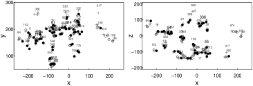
We show the large-scale distribution of rich clusters in superclusters in Fig. 3 in cartesian coordinates. These coordinates are defined as in Park et al. (2007); Liivamägi et al. (2010):

$$\begin{array}[]{l}x=-d\sin\lambda,\\[3.0pt] y=d\cos\lambda\cos\eta,\\[3.0pt] z=d\cos\lambda\sin\eta,\end{array}$$

where $d$ is the comoving distance, and $\lambda$ and $\eta$ are the SDSS survey coordinates. To complement this figure, we present in Appendix C a 3D version of Fig. 3, and the 3D distributions of groups in superclusters with the right ascensions, declinations, and distances of groups.

In Fig. 3 the superclusters SCl 060 and SCl 350 (Table 1) are seen close to us. They belong to the Hercules supercluster, which is split into several superclusters in our sample. These are the nearby rich systems seen in Fig. 2. A chain of poor superclusters connects the Hercules supercluster with rich superclusters at a distance of about 200 $h^{-1}$ Mpc  the superclusters SCl 349 and SCl 351 (the Bootes supercluster) among them. We mentioned in Sect. 2 that at small distances the size of the sample cross-section is only 220x140 $h^{-1}$ Mpc  and these superclusters may be broken up by the sample borders. Therefore the data on nearby superclusters are less reliable than the data on the more distant ones.

Rich superclusters at distances of about 210–260 $h^{-1}$ Mpc form three chains, separated by voids. A 3D figure on our web pages shows that actually only one of these supercluster systems ia a clear chain-like system. This is the Sloan Great Wall (SGW), the richest galaxy system in the nearby Universe (Vogeley et al. 2004; Gott et al. 2005; Nichol et al. 2006; Einasto et al. 2010; Luparello et al. 2011; Pimbblet et al. 2011; Einasto et al. 2011). The SGW consists of several superclusters of galaxies. The richest of them are the superclusters SCl 061 and SCl 024. The other two supercluster chains are much poorer and cannot really be called chains. One of them is separated from the SGW by a void; the Bootes supercluster is the richest supercluster in this system. The richest supercluster in the third system of superclusters is the Ursa Majoris supercluster (SCl 336).

The very rich Corona Borealis supercluster is located at the joint of these systems. This supercluster is a member of a huge system of rich superclusters located at the right angle with respect to the Local Supercluster, described by Einasto et al. (1997b) as the dominant supercluster plane.

At high positive values of the $x$ coordinate there are no rich clusters, and the superclusters in this region are also poor. There are some poor superclusters farther away, perhaps connecting superclusters in our sample volume with more distant superclusters. Thus the large-scale distribution of the superclusters is very inhomogeneous, as noted also in L10.

To make projection effects less significant, we do not show the chains of nearby superclusters in the right panel of Fig. 3. The superclusters SCl 548, SCl 549, SCl 550, SCl 350, and SCl 060 are superimposed on the superclusters SCl 351 and SCl 354, and the superclusters SCl 779 and SCl 796 on the superclusters SCl 038, SCl 336, and SCl 525.

4.2 Morphology of superclusters

The results on the morphology of superclusters are summarised in Table 1 where we list the following morphological characteristics for each supercluster: the maximum value of the fourth Minkowski functional $V_{3,\mathrm{max}}$ (clumpiness), the values of the shapefinders $K_{1}$ (planarity) and $K_{2}$ (filamentarity) for the whole supercluster, and the ratio of the shapefinders $K_{1}$/$K_{2}$ for the whole supercluster. This ratio is not given for the superclusters for which $V_{3}=1$ over the whole mass fraction interval, because the $K_{2}$ may become very small, making the ratio $K_{1}$/$K_{2}$ noisy.

We began the analysis of the structure of superclusters by searching for possible subsets defined by their physical and morphological characteristics. For this purpose we applied the Mclust package for classification and clustering, decribed shortly in Sect. 3.2. Initial data for Mclust was the number of groups with at least 30 member galaxies, the total weighted luminosity of galaxies in a supercluster, its diameter, and the morphological parameters given in Table 1. The results of this analysis show that superclusters can be divided into two main sets. The first set consists of superclusters with shape parameter $K_{1}/K_{2}<0.6$, and second set of those with shape parameter $K_{1}/K_{2}>0.6$ – these superclusters are less elongated than the superclusters in the first set. According to Mclust, the richest supercluster in our sample, the supercluster SCl 061, forms a separate subgroup owing to its very high luminosity. For simplicity, we include this supercluster in the following analysis in the set of more elongated superclusers.

We estimated how well superclusters are assigned to the two different sets using the uncertainity of classification calculated by Mclust (see Sect. 3.2). For our superclusters, the mean uncertainty of the classification is $1.9\cdot 10^{-2}$, showing that superclusters are well classified. To measure how well the sets are determined and to find the best model of a given dataset we use the BIC values given by Mclust. For our sets of superclusters the lowest value of the BIC corresponds to the division of superclusters into two main sets, with SCl 061 forming a separate class. The value of the BIC for the one-component model for superclusters is higher, showing that this model is less likely for our superclusters.

Table 3: Parameters of superclusters in sets according to their morphology.

(1)	(2)	(3)	(4)
	$K_{1}/K_{2}<0.6$		$K_{1}/K_{2}\geq 0.6$
	with SCl 061	without SCl 061
$N_{\mbox{scl}}$	16	15	20
$Distance$	254 $\pm$ 64	254 $\pm$ 66	200 $\pm$ 43
$L_{\mbox{tot}}$	820 $\pm$ 316	790 $\pm$ 274	525 $\pm$ 122
$N_{\mbox{gal}}$	530 $\pm$ 207	442 $\pm$ 176	445 $\pm$ 129
$N_{\mbox{30}}$	2.5 $\pm$ 0.92	2.0 $\pm$ 0.74	2.0 $\pm$ 0.63
$Diameter$	44 $\pm$ 12	43 $\pm$ 11	22 $\pm$ 5
$V_{3}$	4.5 $\pm$ 1.25	4.0 $\pm$ 1.15	2.0 $\pm$ 0.48
$K_{1}$	0.08$\pm$ 0.02	0.08 $\pm$ 0.02	0.03 $\pm$ 0.007
$K_{2}$	0.20$\pm$ 0.05	0.200 $\pm$ 0.05	0.031 $\pm$ 0.008

Figure 4: Shapefinders $K_{1}$ (planarity) and $K_{2}$ (filamentarity) for the superclusters with their clumpiness. The symbol sizes are proportional to the fourth Minkowski functional $V_{3,\mathrm{max}}$. Circles denote superclusters with the shapefinders ratio $K_{1}/K_{2}<0.6$ and squares denote the superclusters with the ratio $K_{1}/K_{2}\geq 0.6$.

Figure 5: Cumulative distributions of the physical characteristics of superclusters for the two sets of superclusters divided by the value of the shape parameter. From left to right: the distributions of luminosities, numbers of galaxies, numbers of rich groups with at least 30 member galaxies, and diameters of superclusters. The black lines correspond to the first set of superclusters with $K_{1}/K_{2}<0.6$, including the supercluster SCl 061, the grey lines to the first set of superclusters without SCl 061, and the dashed lines to the second set of superclusters with $K_{1}/K_{2}>0.6$.

Figure 6: Cumulative distributions of morphological parameters of superclusters for two sets of superclusters divided by the value of the shape parameter. From left to right: the distributions of the fourth Minkowski functional $V_{3}$, of planarities $K_{1}$, and filamentarities $K_{2}$ of superclusters. The black lines correspond to the first set of superclusters with $K_{1}/K_{2}<0.6$, including the supercluster SCl 061, the grey lines to the first set of superclusters without SCl 061, and the dashed lines to the second set of superclusters with $K_{1}/K_{2}>0.6$.

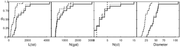
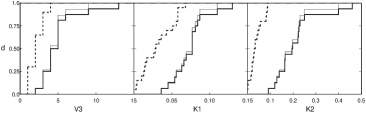
Fig. 4 presents the shapefinders $K_{1}$ (planarity) and $K_{2}$ (filamentarity) in the shapefinder’s plane for our supercluster sample. In this figure circles correspond to those superclusters for which the ratio of the shapefinders $K_{1}/K_{2}<0.6$, and squares to the superclusters with $K_{1}/K_{2}\geq 0.6$, i.e. to more elongated and to less elongated superclusters, respectively. The symbol sizes are proportional to the maximum value of the fourth Minkowski functional $V_{3,\mathrm{max}}$ (clumpiness). This figure reflects both the outer shape and the inner clumpiness (fine structure) of superclusters and summarises the morphological information about superclusters.

Table 1 and Fig. 4 demonstrate that almost all superclusters in our sample are elongated; they have large filamentarities with larger range of values than planarities. Two superclusters with the largest filamentarities and with the ratio of the shapefinders as small as $K_{1}/K_{2}=0.28$ are the most extreme cases of filamentary systems in our sample. These two superclusters are the richest in our sample: SCI 061 and the Corona Borealis. We do not have extremely planar superclusters in our sample ($K_{1}/K_{2}\gg 1.0$). Three superclusters in our sample have $K_{1}/K_{2}\approx 1.0$ (they are spherical), and all these have a small maximum clumpiness ($V_{3,\mathrm{max}}\leq 3$). More elongated superclusters typically have higher values of clumpiness $V_{3}$ than less elongated ones – they have a more complicated morphology (see Table 3).

Figure 7: Shapefinders $K_{1}$ (planarity) and $K_{2}$ (filamentarity), with the luminosities and richnesses of the superclusters. In the left panel symbol sizes are proportional to the total weighted luminosity of galaxies in the superclusters, and in the right panel to the number of galaxies in the superclusters. Circles and squares correspond to two sets of superclusters as in Fig. 4.

Figure 8: Diameters of superclusters (in Mpc/$h$) vs. their shape parameter. Symbol sizes are proportional to the value of the fourth Minkowski functional $V_{3}$ of a supercluster. Circles and squares correspond to the two sets of superclusters as in Fig. 4.

We present the median values of supercluster parameters in these sets in Table 3. In Fig. 5 we plot the cumulative distributions of the values of the physical characteristics of superclusters from the two sets, and in Fig. 6 the cumulative distributions of the morphological parameters. The scatter of the parameters is large, but the superclusters in the first set with the shape parameter $K_{1}/K_{2}<0.6$ (with and without the supercluster SCl 061) are richer, more luminous, and have larger diameters than those in the second set with shape parameter $K_{1}/K_{2}\geq 0.6$. Superclusters from the first set also have higher maximum values of the fourth Minkowski functional $V_{3}$, and higher values of planarities $K_{1}$ and filamentarities $K_{2}$. In Fig. 7 we show another presentation of these results – the shapefinder’s plane for superclusters of different total luminosity and the richness (the number of galaxies in a supercluster) as coded in the symbol sizes explained in figure captions. The two most elongated superclusters are the richest and the most luminous.

Figure 8 and Figure 5 show that more elongated superclusters also have larger diameters than less elongated ones, implying that the systems with larger diameters are not planar structures. Also, there are no compact, planar, and very luminous superclusters.

Table 1 shows that all superclusters with the ratio of shapefinders with $K_{1}/K_{2}\geq 0.6$ are relatively nearby, only four of them lie at distances larger than 250 $h^{-1}$ Mpc. The closest of them is located at about 90 $h^{-1}$ Mpc, and their median distance is about 200 $h^{-1}$ Mpc. As mentioned above, owing to the sample geometry, the nearby superclusters may not be fully included in the sample volume and their small clumpiness may be due to this selection effect. Some nearby poor superclusters are located in low-density filaments between us and more distant superclusters, and their shape and small clumpiness may be real (as noted also in Einasto et al. 1997b). The closest more elongated superclusters with the shape parameter $K_{1}/K_{2}<0.6$ are about 170 $h^{-1}$ Mpc away from us, their mean and median distances almost coincide and are about 254 $h^{-1}$ Mpc (this is approximately the distance to the rich superclusters in the SGW).

Figure 9: Left panels: the distribution of galaxies (grey dots) in the sky, for the two superclusters, SCl 061 (upper row) and SCl 094 (lower row). Circles mark the location of groups with at least 30 member galaxies, and the size of a circle is proportional to the size of a group in the sky. The numbers show Abell clusters. The middle panels show the fourth Minkowski functional $V_{3}$, and the right panels the shapefinders $K_{1}$ (planarity) and $K_{2}$ (filamentarity) for a supercluster. The morphological signature in the $K_{1}-K_{2}$ plane is parametrically defined as $K_{1}(mf)$ and $K_{2}(mf)$. The sizes of open circles are proportional to the value of $V_{3}$ at a given mass fraction $mf$. They show the change of the clumpiness with the mass fraction together with the changes in the morphological signature. The Abell clusters in the supercluster SCl 061 (upper row) are 1 – A1620, 2 – A1650, 3 – A1658, 4 – 1663, 5 – 1682, 6 – 1750, 7 – 1773, 8 – 1780, and 9 – 1809. The Abell clusters in the supercluster SCl 094 (lower row) are 1 – A2067, 2 – A2065, and 3 – A2089.

4.3 Notes on individual superclusters

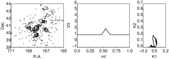
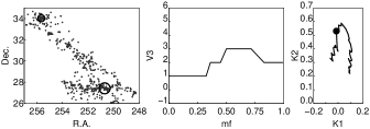
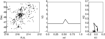
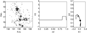
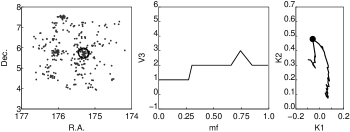
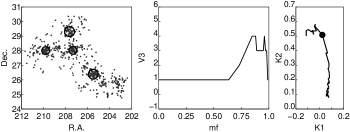
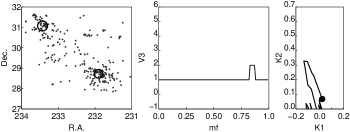
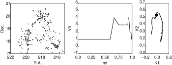
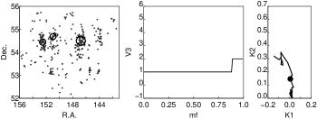
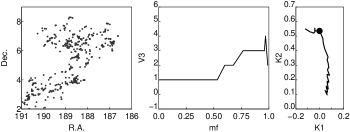
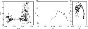
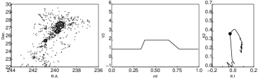
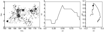
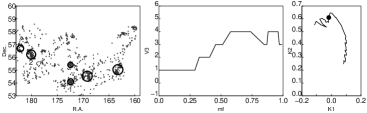
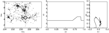
Below, we give a short description of individual superclusters in our sample. In the figures of this section and in Appendix D we show for each supercluster (except for those for which $V_{3}=1$ over the whole mass fraction interval) the sky distribution of supercluster members, the values of the fourth Minkowski functional $V_{3}$ vs. the mass fraction $mf$ and the morphological signature for each supercluster. Panels in these figures are as follows. The left panels show the sky distributions of galaxies in superclusters and the location of rich groups with at least 30 member galaxies. The middle panels show the clumpiness $V_{3}$ vs. the mass fraction $mf$ for a whole mass fraction interval from 0 to 1, and the right panels the shapefinder’s $(K_{1},K_{2})$ curve (the morphological signature) for a supercluster. The mass fraction increases anti-clockwise along the curves. In these panels the value of mass fraction $mf=0.7$ is marked – at this value the morphological signature of rich superclusters changes. We will classify our superclusters as spiders, multispiders, filaments, and multibranching filaments on the basis of their morphological information and visual appearance. Often superclusters are of intermediate type between these main types, hence for some superclusters our classification is a suggestion only.

We begin with the two richest superclusters from our sample (Fig. 9). For these two superclusters the morphological signature (Fig. 9, right panels) is plotted with symbols of the size proportional to the value of the fourth Minkowski functional $V_{3}$ at a given mass fraction, to show how the morphological signature changes together with the changes in clumpiness, as described in Sect. 3.1. Here we do not mark the value of mass fraction $mf=0.7$, for clarity.

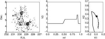
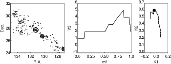
The supercluster SCl 061 at a distance of 256 $h^{-1}$ Mpc is the richest member of the SGW (Einasto et al. 2011; Luparello et al. 2011). This supercluster contains nine Abell clusters, the largest number in our sample. Five of these are also X-ray clusters (Böhringer et al. 2004). The richest of them, A1750, is a merging X-ray cluster (Belsole et al. 2004). The morphology of SCl 061 resembles a multibranching filament with the maximum value of the fourth Minkowski functional $V_{3,\mathrm{max}}=13$, and the ratio of the shapefinders $K_{1}$/$K_{2}=0.28$, one of the lowest in our catalogue (Fig. 9, upper row, and Table 1).

The supercluster SCl 094 (the Corona Borealis supercluster) at a distance of 215 $h^{-1}$ Mpc is the second in richness among our sample. This system contains three Abell clusters (A2067, A2065, and A2089), and is a member of the dominant supercluster plane (Einasto et al. 1997b). The distribution of galaxies in the sky in SCl 094 is plotted in Fig. 9 (lower row, left panel). The maximum value of the fourth Minkowski functional of the Corona Borealis supercluster $V_{3,\mathrm{max}}=10$, and the ratio of the shapefinders $K_{1}$/$K_{2}=0.28$ (Fig. 9, the middle and right panels of the lower row, and Table 1). Morphologically SCl 094 is a multispider with a number of clusters connected by low density filaments, with an overall very elongated shape that resembles a horse-shoe, with the merging X-ray cluster A2065 at the top (Chatzikos et al. 2006). SCl 094 has been studied by Small et al. (1998), who found that the core of this system probably has started to collapse. Numerical simulations show that such collapsing cores in superclusters are rare (Gramann & Suhhonenko 2002). Luparello et al. (2011) proposed that SCl 094 may merge with several surrounding superclusters in the future. In last years interest in the Corona Borealis supercluster region has grown because of the discovery of the CMB cold spot in it’s direction. This may be partly caused by the warm-hot diffuse gas in the supercluster filaments between the clusters, or by some undiscovered distant cluster (Génova-Santos et al. 2008; Padilla-Torres et al. 2009; Génova-Santos et al. 2010; Padilla-Torres et al. 2010, and references therein). The poor superclusters SCl 362 and SCl 366 are also members of the Corona Borealis supercluster. The morphology of SCl 362 resembles a simple spider with the ratio of the shapefinders $K_{1}$/$K_{2}=1.0$, while that of SCl 366 resembles a multibranching filament with the maximum value of the fourth Minkowski functional $V_{3,\mathrm{max}}=4$, and the ratio of the shapefinders $K_{1}$/$K_{2}=0.38$ (Fig. 17).

The supercluster SCl 001 contains two rich Abell clusters, A2142 and A2149, both of them are X-ray sources (Table 2). Chandra observations have revealed that A2142 is probably still merging (Markevitch et al. 2000). SCl 001 is located in a region with a dense concentration of superclusters, close to SCl 011 and SCl 094. All these systems form a part of the dominant supercluster plane. At the location of SCl 001 the luminosity density is the highest in the whole SDSS survey; this is probably at least partly because of the rich X-ray cluster A2142. The morphology of SCl 001 resembles a filament where clusters are located almost along a straight line (the 3D model on our web pages shows this best). The maximum value of the fourth Minkowski functional for SCl 001 $V_{3,\mathrm{max}}=2$ and the ratio of the shapefinders $K_{1}$/$K_{2}=0.48$ (Fig. 10 and Table 1).

Figure 10: Panels as in Fig. 9. Filled circles in the right panel mark the value of the mass fraction $mf=0.7$. Upper row: the supercluster SCl 001. The Abell clusters are 1 – A2142 and 2 – A2149. Middle row: the supercluster SCl 011. The Abell clusters are 1 – A2040 and 2 – A2028. Lower row: the supercluster SCl 024. The Abell clusters are 1 – A1424 and 2 – A1516.

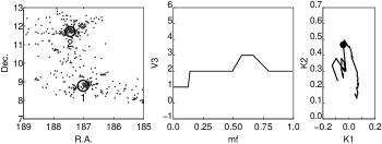
The supercluster SCl 011 at a distance of 234 $h^{-1}$ Mpc contains two Abell clusters, A2040 and A2028, which are members of different superclusters in E01. The maximum value of the fourth Minkowski functional $V_{3,\mathrm{max}}=3$ (Fig. 10, middle row), the ratio of the shapefinders $K_{1}$/$K_{2}=0.92$. The morphology of SCl 011 resembles a sparse multispider or multibranching filament with a quite uniform density (as suggested by the low values of the fourth Minkowski functional $V_{3}$ for a wide mass fraction interval). SCl 011 belongs to the same supercluster complex as SCl 001 (Fig. 3).

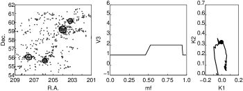
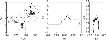
The supercluster SCl 024 at a distance of 230 $h^{-1}$ Mpc is the second richest member of the SGW. SCl 024 contains two Abell clusters, A1424 and A1516. Its morphology resembles a multispider with the maximum value of the fourth Minkowski functional $V_{3,\mathrm{max}}=5$ and the ratio of the shapefinders $K_{1}$/$K_{2}=0.48$ (Fig. 10, lower row). The values of the fourth Minkowski functional of SCl 024 at small mass fractions ($mf\approx 0.25$) $V_{3}=0$ suggest that SCl 024 has low-density tunnels inside (Einasto et al. 2011). The member of the supercluster SCl 111 in E01 to which SCl 024 also belong, the poor supercluster SCl 223, can be described as a multispider with two concentrations –the fourth Minkowski functional has a value of 2 for a wide mass fraction interval (Fig. 16). SCl 223 is separated from SCl 024 and SCl 055 by a small void, showing that clusters gathered together into one supercluster in the E01 catalogue sometimes do not belong to the same supercluster, when systems are determined using data on galaxies.

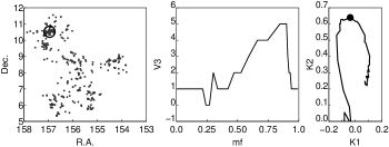
The supercluster SCl 055 at a distance of 242 $h^{-1}$ Mpc  is separated from the SGW by a void and is connected to it by a filament of galaxies (this is the reason why SCl 024 and SCl 055 both belong to the supercluster SCl 111 in the E01 catalogue). SCl 055 contains one Abell cluster, A1358. The morphology of SCl 055 resembles a multibranching filament or an elongated multispider with the maximum value of the fourth Minkowski functional $V_{3,\mathrm{max}}=5$ and the ratio of the shapefinders $K_{1}$/$K_{2}=0.43$ (Fig. 11).

Figure 11: Panels are the same as in Fig. 9. Upper row: the supercluster SCl 055. The Abell cluster is A1358. Middle row: the supercluster SCl 336. The Abell clusters are 1 – A1279, 2 – A1436. Lower row: the supercluster SCl 350. The Abell clusters are 1 – A2052, 2 – A2063.

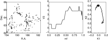
The supercluster SCl 336 contains two Abell clusters, A1279 and A1436, which are members of the Ursa Majoris supercluster (Fig. 11, middle row). SCl 336 belongs to a chain of superclusters that is separated by a void from SCl 349 and SCl 351 (the Bootes supercluster) (see also Kopylova & Kopylov 2009, and references therein). Luparello et al. (2011) found that several filamentary systems may be associated with this system. According to our calculations, the morphology of the Ursa Majoris supercluster resembles a sparse multibranching filament with the maximum value of the fourth Minkowski functional $V_{3,\mathrm{max}}=4$, and the ratio of the shapefinders $K_{1}$/$K_{2}=0.33$ (Fig. 11). The poor supercluster SCl 525 is also a member of the Ursa Majoris supercluster, morphologically SCl 525 can be described as a spider.

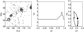
The superclusters SCl 010, SCl 060, and SCl 350 belong to the rich Hercules supercluster that is split between several systems in our present catalogue. They are located at a distance of about 100 $h^{-1}$ Mpc and contain clusters that are exceptionally rich in the T10 catalogue, owing to their small distance from us (A2152 in SCl 010 and A2197 in SCl 060). This is the reason why the value of the fourth Minkowski functional for SCl 010 and SCl 060 $V_{3}=1$ over the whole mass fraction interval, showing that they contain only one high density clump. SCl 350 contains five rich clusters, three of them correspond to the Abell cluster A2052. This suggests that A2052 has a substructure, with different components corresponding to different groups and clusters in the T10 catalogue. The maximum value of the fourth Minkowski functional for SCl 350, $V_{3,\mathrm{max}}=2$ (Fig. 11, lower row), and the ratio of the shapefinders $K_{1}$/$K_{2}=0.65$. At the farther end SCl 350 chain joins the dominant supercluster plane (Fig. 3).

We summarise the results of the morphological analysis of the superclusters in Table 4. For clarity we present the figures of the distribution of galaxies and rich groups/clusters in the sky for superclusters with less than 950 members galaxies, as well as their fourth Minkowski functionals and the morphological signatures in Appendix D.

Table 4: Data of the morphology of superclusters.

(1)	(2)	(3)	(4)	(5)	(6)	(7)	(8)	(9)
$SCl_{ID}$	$d_{\mbox{peak}}$	$N_{\mbox{gal}}$	$N_{\mbox{30}}$	$N_{\mbox{Abell}}$	$V_{3,\mathrm{max}}$	Set	$Morph.$	Notes
	Mpc/$h$
1	264.5	1038	4	2	2	1	F
10	111.9	1463	2	1	1	2	S
11	235.0	1222	5	2	3	2	mS(mF)
24	230.4	1469	4	2	6	1	mS	SGW
55	242.0	1306	4	1	5	1	mS(mF)
60	92.0	1335	3	1	1	2	S
61	255.6	3056	15	9	13	1	mF	SGW
94	215.4	1830	10	3	9	1	mS
336	170.0	1005	6	2	4	1	mF
350	105.8	955	5	2	2	2	mS
38	224.4	586	5	2	2	2	S
64	301.7	619	2	2	3	1	F
87	213.4	445	1	1	2	2	S
136	212.1	504	5	1	2	2	S
152	301.6	423	2	2	3	2	F
189	267.2	433	1	0	4	1	F
198	284.7	473	1	1	4	2	mF
223	268.3	462	2	2	3	1	mS
228	210.6	643	4	1	2	2	F
317	321.6	351	1	0	5	1	mS	T
332	291.0	333	1	1	3	2	mS
349	188.0	893	5	3	5	1	mS	F(L11)
351	225.4	615	4	3	4	2	mF
362	195.2	306	2	3	2	2	mS
366	300.4	353	0	0	4	1	mF
376	258.7	437	2	1	3	2	F	T
474	251.2	389	3	1	5	1	F
512	227.7	371	2	2	3	1	mF
525	154.2	438	4	2	3	2	mS
530	306.8	333	0	0	5	1	mS	T
548	158.7	314	2	1	1	2	S	Her-DSP
549	162.5	322	1	0	1	2	S	Her-DSP
550	135.1	459	3	2	1	2	S	Her-DSP
779	139.7	353	1	0	2	2	mS	SGW chain
796	102.3	369	1	1	1	2	S	SGW chain
827	254.1	405	0	0	4	1	F

In Table 4 we list for every supercluster their distance, the numbers of galaxies, the number of rich groups with at least 30 member galaxies, and the number of Abell clusters among them. From morphological parameters we list the maximum value of the fourth Minkowski functional and the number that shows whether the supercluster belongs to the set 1 (more elongated superclusters) or to the set 2 (less elongated superclusters). We also give morphological descriptions of superclusters and notes.

Table 4 shows that superclusters with a smaller number of galaxies also contain, as expected, a smaller number of rich groups and Abell clusters. Among them less elongated superclusters dominate over more elongated superclusters – there are 16 systems from set 2 and 10 from set 1 among them. The morphology of 14 of them can be described as simple spider or simple filament, and 12 of them are either multispiders or multibranching filaments. In contrast, of 10 superclusters with at least 950 member galaxies 7 can be described as multispiders of multibranching filaments, two of them are simple spiders and one is a simple filament.

5 Discussion

5.1 Selection effects

The main selection effect in our study comes from the use of the flux-limited sample of galaxies to determine the luminosity density field and superclusters. To keep the luminosity-dependent selection effects as small as possible, we used data on galaxies and galaxy systems for a distance interval 90–320 $h^{-1}$ Mpc. In this interval these effects are the smallest (we refer to T10 for details). We calculate Minkowski functionals of individual superclusters from volume limited samples. This approach makes the calculations of morphology insensitive to luminosity dependent selection effects.

Another selection effect comes from the choice of the density level used to determine superclusters. At the density level applied in the present paper ($D=5.0$), rich superclusters do not percolate yet. For example, in the SGW we see several individual rich superclusters. At a lower threshold density these superclusters join into a huge system. In the same time the Corona Borealis supercluster is split into several superclusters in our catalogue at the density level $D=5.0$ . Thus there is no unique density level, which would be the best choice for all superclusters. However, L10 show that superclusters are fairly well-defined systems and do not change much when changing the density level, if only this change is small and does not break them up into small systems or does not join them into huge percolating systems. When we move towards higher density levels, some galaxies and galaxy systems in the lower density outskirts of a supercluster do not belong to the supercluster any more; in that case the clumpiness of the supercluster at low mass fractions may decrease. Moving towards lower density levels, new galaxies and galaxy systems in the outskirts of a supercluster become supercluster members. This may increase the value of the clumpiness and change the morphological signature of a supercluster at low mass fractions. The possible change in morphology depends on the number of galaxies and on the richness of groups removed from or added to the supercluster and is individual for each supercluster.

At small distances our sample volume is small, which introduces another selection effect – nearby rich superclusters are split between several superclusters, some parts of these superclusters may be located outside of the sample volume. This makes the data about nearby superclusters less reliable.

The identification of Abell clusters may also be affected by selection effects. It is well known that some Abell clusters consist of several line-of-sight components. A good example of such a cluster is the cluster Abell 1386, recently studied by Pimbblet et al. (2011). Our search discarded Abell clusters affected by this projection effect.

5.2 Comparison with other studies

Recently Costa-Duarte et al. (2011) used volume-limited samples of galaxies from the SDSS DR7 to extract superclusters of galaxies and to study the morphology of whole superclusters with the shape parameter (the ratio of the shapefinders $K_{1}/K_{2}$). To determine superclusters the authors calculated the density field with an Epanechnikov kernel and found systems of galaxies with at least 10 member galaxies. In Einasto et al. (2007d), we compared the Epanechnikov and $B_{3}$ box spline kernels and found that both kernels are good to describe the overall shape of superclusters, while the $B_{3}$ box spline kernel better resolves the inner structure of superclusters. This is the reason why we used this kernel in the present study. The most important difference between our studies is that we used the data about the richer superclusters with at least 300 member galaxies. Costa-Duarte et al. (2011) showed that there are both planar and filament-like superclusters (pancakes and filaments) among the superclusters of their sample, while in our sample there are almost no superclusters for which planarity is larger than filamentarity. However, Costa-Duarte et al. (2011) found that very rich and luminous superclusters tend to be filaments, as we also found in our study.

The overall shapes of superclusters, described by the shape parameters or approximated by triaxial ellipses, have been analysed in Jaaniste et al. (1998); Kolokotronis et al. (2002); Basilakos (2003); Einasto et al. (2007a); Costa-Duarte et al. (2011); Luparello et al. (2011). These studies showed that elongated, prolate structures dominate among superclusters, as we also found in our study. In the analysis of the geometry of the structures around the galaxy clusters from simulations Noh & Cohn (2011) showed that these structures tend to lie on planes. Similarly, in our study and in the study by Costa-Duarte et al. (2011) poorer systems are more planar. Sheth et al. (2003) used the shapefinders plane $K_{1}$-$K_{2}$ (the morphological signature in our study) to study the morphology of superclusters in simulations. They found that richer and more massive superclusters tend to be more filamentary and have a more complicated inner structure (high values of the genus in their study).

Future evolution of the structure in the Universe has been addressed in simulations by several authors, we refer to Araya-Melo et al. (2009) for a review and references. Araya-Melo et al. (2009) studied the evolution of the shape and inner structure of superclusters in simulations from the present time to a distant future (from $a=1$ to $a=100$, $a$ is the expansion factor). In their study superclusters were defined as high-mass bound objects, and the supercluster shape was approximated by triaxial ellipses. To analyse the substructure of superclusters they used the multiplicity function of clusters in superclusters. Araya-Melo et al. (2009) showed that superclusters are elongated, prolate structures, there are no thin pancakes among them. Future superclusters are typically much more spherical than present-day superclusters. Presently, the superclusters contain a large number of clusters, which may merge into a single cluster in the far future, i.e., multispiders and multibranching filaments may evolve into simple spiders and filaments.

Comparisons of the properties of rich and poor superclusters have revealed several differences between them. The mean and maximum number densities of galaxies in rich superclusters are higher than in poor superclusters. Rich superclusters are more asymmetrical than poor superclusters (Einasto et al. 2007a). Rich superclusters contain high-density cores (Einasto et al. 2007c). The fraction of rich clusters and X-ray clusters in rich superclusters is larger than in poor superclusters (Einasto et al. 2001; Luparello et al. 2011), and the core regions of the richest superclusters may contain merging X-ray clusters (Bardelli et al. 2000; Rose et al. 2002). However, we still lack a detailed analysis of whether the differences between the properties of the galaxy and group content of rich and poor superclusters are related also to the differences in morphology of superclusters.

In Einasto et al. (2008) we compared the properties of the two richest superclusters from the 2dF Galaxy Redshift Survey, the superclusters SCl 126 (SCl 061 in the present study), and the Sculptor supercluster (SCl 9 in E01). We used Minkowski functionals to quantify the fine structure of these superclusters as traced by different galaxy populations. Our calculations showed that in the supercluster SCl 126 the population of red, early type galaxies is more clumpy than the population of blue, late type galaxies, especially in the outskirts of the supercluster. In contrast, in the supercluster SCl 9 the clumpiness of galaxies of different type is quite similar in its outskirts. In the core of the supercluster SCl 9 the clumpiness of blue, late type galaxies is larger than the clumpiness of red, early type galaxies. In the supercluster SCl 111 in the SGW the clumpiness of red galaxies is larger than that of blue galaxies (Einasto et al. 2011). Morphologically the supercluster SCl 126 resembles a multibranching filament, while the Sculptor supercluster and SCl 111 resemble a multispider. We need to study the morphology and galaxy populations of a larger sample of superclusters to find out whether the differences between galaxy populations in superclusters are also related to their different morphology.

Aragón-Calvo et al. (2010) recently studied the structure and morphologies of elements that define the cosmic web with the Multiscale Morphology Filter and data from $\Lambda$CDM simulations. The authors found several typical morphologies for filaments, which they describe as line, grid, star, and complex filaments. We can compare that with our classification of supercluster morphologies. Approximately, line filaments are comparable with our simple filaments. Star filaments can be compared with simple spiders. Grid and complex filaments may correspond either to multibranching filaments or to multispiders, although complex filaments are more similar to multispiders and grid filaments to multibranching filaments. This shows that the morphology of observed and simulated superclusters is, in general, similar, as we found earlier from much smaller samples of observed and simulated superclusters. The biggest exception is the supercluster SCl 061, a very rich and high-density multibranching filament. No other supercluster with such a morphology has been found yet either in simulations in observations (see also Gott et al. 2008). Another difference between the observed and simulated superclusters, as quantified by Minkowski functionals and shapefinders, is fine structure of superclusters, delineated by galaxies of different luminosity (Einasto et al. 2007d). The clumpiness of observed superclusters for galaxies of different luminosity has a much larger scatter than that of simulated superclusters. Simulations do not yet explain all the features of observed superclusters.

6 Summary and conclusions

We have presented an analysis of the large-scale distribution and morphology of superclusters from the SDSS DR7. While the overall shape of superclusters has been analysed earlier in several studies, our paper is the first in which the inner morphology of a large sample of observed superclusters is studied in detail. We used multidimensional normal mixture modelling to divide superclusters into two sets according to their physical and morphological properties. We present 2D and 3D distributions of galaxies and rich groups in superclusters, the clumpiness curve (the fourth Minkowski functional $V_{3}-mf$ relation), as well as the morphological signature $K_{1}$-$K_{2}$ for each supercluster in our sample .

The superclusters were selected to contain at least 300 observed galaxies. As we showed, this does not mean that all superclusters in our sample are rich – about 1/4 of our superclusters contain one rich cluster or group only (three superclusters do not contain any rich group or cluster).

Summarising, our study showed that:

• Most superclusters contain Abell clusters, about 1/3 of them are X-ray clusters.

• The large-scale distribution of the superclusters is very inhomogeneous. Rich superclusters in the sample form three chains, the Sloan Great Wall is the richest of them.

• Almost all superclusters under study are elongated and have filamentarities that are larger than than their planarities. More elongated superclusters are also more luminous, have larger diameters and contain a larger number of rich clusters. The values of the fourth Minkowski functional $V_{3}$ show that they also have a more complicated inner morphology than less elongated superclusters.

• The morphological analysis shows a large variety of morphologies among superclusters. The fine structure of superclusters can be described with four main types of morphology: spiders, multispiders, filaments, and multibranching filaments. Often a supercluster has an intermediate morphology between these main types. Superclusters with a similar shape parameter may have a different fine structure. Consequently neither the shape parameter or the number of rich clusters in a supercluster alone are sufficient to describe the morphology of superclusters.

Our results on the morphology of superclusters can be used to compare the properties of local and high-redshift superclusters. Few superclusters at very high redshifts have already been discovered in deep, wide-field imaging surveys (Nakata et al. 2005; Swinbank et al. 2007; Gal et al. 2008; Tanaka et al. 2009; Schirmer et al. 2011). Deep surveys like the ALHAMBRA project (Moles et al. 2008) will provide us with data about (possible) very distant superclusters; we can analyse their structure and compare that with the local superclusters, using morphological methods.

Our study does not give a definite answer to the question about the possible connection between the morphology of superclusters and their large-scale distribution. Also, there are superclusters in our sample that can be described as filaments or multibranching filaments, but none of them is as rich and has such an overall high density as the supercluster SCl 061. Even the richest supercluster with a multispider morphology in our sample, the supercluster SCl 094, is not as rich as the very rich Sculptor supercluster in Einasto et al. (2007d). This shows the need for a larger sample of superclusters to understand the morphological variety of superclusters, and to study the possible connection between the large-scale distribution of superclusters and their morphology.

Different morphologies of superclusters suggest that their evolution has been different. To understand the formation and evolution of superclusters of different morphology better, we need to study the properties and evolution of superclusters in simulations. The morphology of superclusters and its evolution may be one of the factors to distinguish between different cosmological models (Kolokotronis et al. 2002; Hoffman et al. 2007). Especially interesting is the supercluster SCl 061 in the Sloan Great Wall. Up to now simulations have not been able to model its morphology (Einasto et al. 2007d, and references therein). New simulations with larger volumes are needed to study the morphology of superclusters and the evolution of the morphology of simulated superclusters, to understand the reasons for the exceptional morphology of the supercluster SCl 061. In addition, very rich superclusters are rare; another reason to use simulations for large volumes comes from the demand to include as large a variety of superclusters in the simulation volume as possible.

Appendix A Luminosity density field and superclusters

To calculate the luminosity density field, we must first calculate the luminosities of groups. In flux-limited samples galaxies outside the observational window remain unobserved, and we have also to take into account the luminosities of these galaxies as well. For that, we multiply the observed galaxy luminosities by the luminosity weight $W_{d}$. The distance-dependent weight factor $W_{d}$ was calculated as follows:

$$W_{d}={\frac{\int_{0}^{\infty}L\,n(L)\mathrm{d}L}{\int_{L_{1}}^{L_{2}}L\,n(L)\mathrm{d}L}},$$ (1)

where $L_{1,2}=L_{\sun}10^{0.4(M_{\sun}-M_{1,2})}$ are the luminosity limits of the observational window at a distance $d$, corresponding to the absolute magnitude limits of the survey $M_{1}$ and $M_{2}$; we took $M_{\sun}=4.64$ mag in the $r$-band (Blanton & Roweis 2007). Owing to their peculiar velocities, the distances of galaxies are somewhat uncertain; if the galaxy belongs to a group, we used the group distance to determine the weight factor.

To calculate a luminosity density field, we converted the spatial positions of galaxies $\mathbf{r}_{i}$ and their luminosities $L_{i}$ into spatial (luminosity) densities. For that we use kernel densities (Silverman 1986):

$$\rho(\mathbf{r})=\sum_{i}K\left(\mathbf{r}-\mathbf{r}_{i};a\right)L_{i},$$ (2)

where the sum is over all galaxies, and $K\left(\mathbf{r};a\right)$ is a kernel function of a width $a$. Good kernels for calculating densities on a spatial grid are generated by box splines $B_{J}$. Box splines are local and they are interpolating on a grid:

$$\sum_{i}B_{J}\left(x-i\right)=1,$$ (3)

for any $x$ and a small number of indices that give non-zero values for $B_{J}(x)$. We used the popular $B_{3}$ spline function:

$$B_{3}(x)=\frac{1}{12}\left(|x-2|^{3}-4|x-1|^{3}+6|x|^{3}-4|x+1|^{3}+|x+2|^{3}\right).$$ (4)

We defined the (one-dimensional) $B_{3}$ box spline kernel $K_{B}^{(1)}$ of the width $a$ as

$$K_{B}^{(1)}(x;a,\delta)=B_{3}(x/a)(\delta/a),$$ (5)

where $\delta$ is the grid step. This kernel differs from zero only in the interval $x\in[-2a,2a]$; it is close to a Gaussian with $\sigma=1$ in the region $x\in[-a,a]$, so its effective width is $2a$ (see, e.g., Saar 2009). The kernel exactly preserves the interpolation property for all values of $a$ and $\delta$, where the ratio $a/\delta$ is an integer. (This kernel can be used also if this ratio is not an integer, and $a\gg\delta$; the kernel sums to 1 in this case, too, with a very small error). This means that if we apply this kernel to $N$ points on a one-dimensional grid, the sum of the densities over the grid is exactly $N$.

The three-dimensional kernel $K_{B}^{(3)}$ is given by the direct product of three one-dimensional kernels:

$$K_{B}^{(3)}(\mathbf{r};a,\delta)\equiv K_{3}^{(1)}(x;a,\delta)K_{3}^{(1)}(y;a,\delta)K_{3}^{(1)}(z;a,\delta),$$ (6)

where $\mathbf{r}\equiv\{x,y,z\}$. Although this is a direct product, it is isotropic to a good degree (Saar 2009).

The densities were calculated on a cartesian grid based on the SDSS $\eta$, $\lambda$ coordinate system, because it allowed the most efficient fit of the galaxy sample cone into a brick. Using the rms velocity $\sigma_{v}$, translated into distance, and the rms projected radius $\sigma_{r}$ from the group catalogue (T10), we suppressed the cluster finger redshift distortions. We divided the radial distances between the group galaxies and the group centre by the ratio of the rms sizes of the group finger:

$$d_{\mathrm{gal,f}}=d_{\mathrm{group}}+(d_{\mathrm{gal,i}}-d_{\mathrm{group}})\;\sigma_{\mathrm{r}}/\sigma_{\mathrm{v}}.$$ (7)

This removes the smudging effect the fingers have on the density field. We used an 1 $h^{-1}$ Mpc step grid and chose the kernel width $a=8$ $h^{-1}$ Mpc. This kernel differs from zero within the radius 16 $h^{-1}$ Mpc, but significantly so only inside the 8 $h^{-1}$ Mpc radius.

Before extracting superclusters we applied the DR7 mask constructed by P. Arnalte-Mur (Martínez et al. 2009; Liivamägi et al. 2010) to the density field and converted densities into units of mean density. The mean density is defined as the average over all pixel values inside the mask. The mask is designed to follow the edges of the survey and the galaxy distribution inside the mask is assumed to be homogeneous.

Appendix B Minkowski functionals and shapefinders

For a given surface the four Minkowski functionals (from the first to the fourth) are proportional to the enclosed volume $V$, the area of the surface $S$, the integrated mean curvature $C$, and the integrated Gaussian curvature $\chi$. Consider an excursion set $F_{\phi_{0}}$ of a field $\phi(\mathbf{x})$ (the set of all points where the density is higher than a given limit, $\phi(\mathbf{x}\geq\phi_{0}$)). Then, the first Minkowski functional (the volume functional) is the volume of this region (the excursion set):

$$V_{0}(\phi_{0})=\int_{F_{\phi_{0}}}\mathrm{d}^{3}x\;.$$ (8)

The second Minkowski functional is proportional to the surface area of the boundary $\delta F_{\phi}$ of the excursion set:

$$V_{1}(\phi_{0})=\frac{1}{6}\int_{\delta F_{\phi_{0}}}\mathrm{d}S(\mathbf{x})\;,$$ (9)

(but it is not the area itself, notice the constant). The third Minkowski functional is proportional to the integrated mean curvature $C$ of the boundary:

$$V_{2}(\phi_{0})=\frac{1}{6\pi}\int_{\delta F_{\phi_{0}}}\left(\frac{1}{R_{1}(\mathbf{x})}+\frac{1}{R_{2}(\mathbf{x})}\right)\mathrm{d}S(\mathbf{x})\;,$$ (10)

where $R_{1}(\mathbf{x})$ and $R_{2}(\mathbf{x})$ are the principal radii of curvature of the boundary. The fourth Minkowski functional is proportional to the integrated Gaussian curvature (the Euler characteristic) of the boundary:

$$V_{3}(\phi_{0})=\frac{1}{4\pi}\int_{\delta F_{\phi_{0}}}\frac{1}{R_{1}(\mathbf{x})R_{2}(\mathbf{x})}\mathrm{d}S(\mathbf{x})\;.$$ (11)

At high (low) densities this functional gives us the number of isolated clumps (void bubbles) in the sample (Martínez & Saar 2002; Saar et al. 2007):

$$V_{3}=N_{\mbox{clumps}}+N_{\mbox{bubbles}}-N_{\mbox{tunnels}}.$$ (12)

As the argument labelling the isodensity surfaces, we chose the (excluded) mass fraction $mf$ – the ratio of the mass in the regions with the density lower than the density at the surface, to the total mass of the supercluster. When this ratio runs from 0 to 1, the iso-surfaces move from the outer limiting boundary into the centre of the supercluster, i.e., the fraction $mf=0$ corresponds to the whole supercluster, and $mf=1$ – to its highest density peak.

We used directly only the fourth Minkowski functional in this paper; the other functionals were used to calculate the shapefinders (Sahni et al. 1998; Shandarin et al. 2004; Saar 2009). The shapefinders are defined as a set of combinations of Minkowski functionals: $H_{1}=3V/S$ (thickness), $H_{2}=S/C$ (width), and $H_{3}=C/4\pi$ (length). The shapefinders have dimensions of length and are normalized to give $H_{i}=R$ for a sphere of radius $R$. For smooth (ellipsoidal) surfaces, the shapefinders $H_{i}$ follow the inequalities $H_{1}\leq H_{2}\leq H_{3}$. Oblate ellipsoids (pancakes) are characterised by $H_{1}<<H_{2}\approx H_{3}$, while prolate ellipsoids (filaments) are described by $H_{1}\approx H_{2}<<H_{3}$.

Sahni et al. (1998) also defined two dimensionless shapefinders $K_{1}$ (planarity) and $K_{2}$ (filamentarity): $K_{1}=(H_{2}-H_{1})/(H_{2}+H_{1})$ and $K_{2}=(H_{3}-H_{2})/(H_{3}+H_{2})$.

In the $(K_{1},K_{2})$-plane filaments are located near the $K_{2}$-axis, pancakes near the $K_{1}$-axis, and ribbons along the diameter, connecting the spheres at the origin with the ideal ribbon at $(1,1)$. In Einasto et al. (2007d) we calculated typical morphological signatures of a series of empirical models that serve as morphological templates to compare with the characteristic curves for superclusters in the $(K_{1},K_{2})$-plane.

Appendix C 3D figures of superclusters

Here we show the 3D distribution of groups in our superclusters. Figure 12 is 3D presentation of Fig. 3 and shows the distribution of groups with at least twelve member galaxies in our superclusters in the cartesian coordinates defined in Section 4.1, in units of $h^{-1}$ Mpc. The filled circles denote groups with at least 50 member galaxies, empty circles denote groups with 30–49 member galaxies and crosses denote groups with 12–29 member galaxies. The numbers are ID numbers of superclusters with at least 950 member galaxies. Fig. 13,  15, and  15 show 3D distribution of groups in superclusters. In these figures we plot rich groups with at least 30 member galaxies with filled circles, groups with 2 – 29 member galaxies with empty circles. We do not show the figures for superclusters, for which the value of the fourth Minkowski functional $V_{3}=1$ over the whole mass fraction interval.

Figure 12: Distribution of groups with at least 12 member galaxies in our superclusters in the cartesian coordinates as in Fig. 3, in units of $h^{-1}$ Mpc. Filled circles denote the groups with at least 50 member galaxies, empty circles denote the groups with 30–49 member galaxies and crosses denote the groups with 12–29 member galaxies. The numbers show the ID’s (Table 1, column 1) of very rich superclusters from Sect. 4.3.

Figure 13: 3D figures of the very rich superclusters described in Sect. 4.3. Filled circles show the location of rich groups and clusters with at least 30 member galaxies, empty circles show poorer groups. We plot the right ascension (in degrees), declination (in degrees), and distance (in Mpc/$h$) of groups. Plots of superclusters are given in the same order as they are presented in the text. From top to bottom: left: the supercluster SCl 061, right: SCl 094, left: the supercluster SCl 001, right: SCl 011, left: the supercluster SCl 024, right: SCl 055, left: the supercluster SCl 336, right: SCl 350.

Figure 14: 3D figures of superclusters with less than 950 member galaxies. Panels and notations in this figure are the same as in Fig. 13. From top to bottom: left: the supercluster SCl 038, right: SCl 064, left: the supercluster SCl 087, right: SCl 136, left: the supercluster SCl 152, right: SCl 189, left: the supercluster SCl 198, right: SCl 223, left: the supercluster SCl 228, right: SCl 317, left: the supercluster SCl 332, right: SCl 349, left: the supercluster SCl 351, right: SCl 362, left: the supercluster SCl 366, right: SCl 376.

Figure 15: 3D figures of superclusters with less than 950 member galaxies (continued). Panels and notations in this figure are the same as in Fig. 13. From top to bottom: left: the supercluster SCl 474, right: SCl 512, left: the supercluster SCl 525, right: SCl 530, left: the supercluster SCl 779, right: SCl 827.

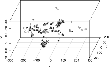
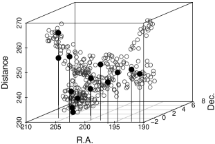
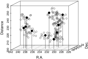
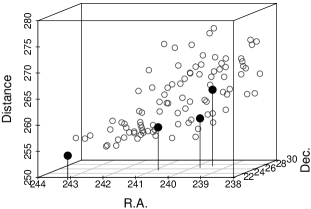
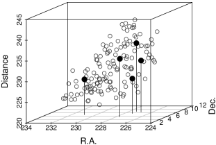
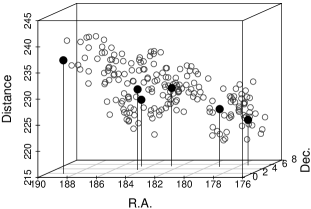
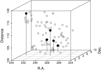
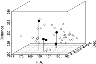
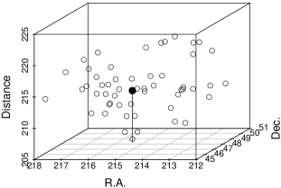
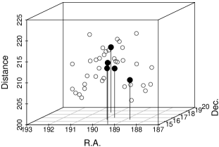
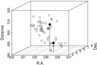
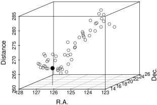
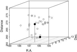
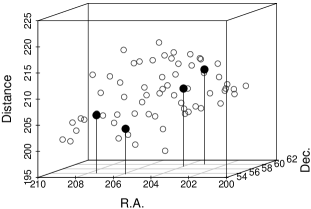
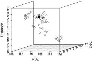
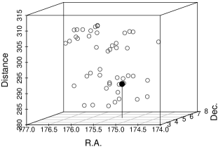
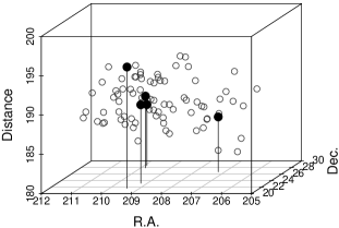
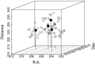
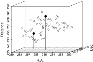
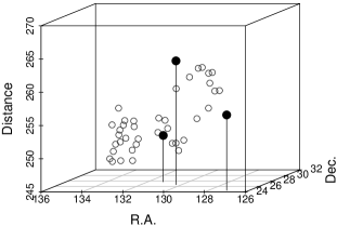
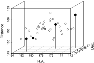
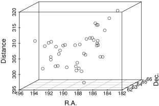
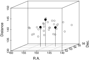
Appendix D The distribution of galaxies and rich groups in the sky and the fourth Minkowski functional and morphological signature for superclusters with less than 950 member galaxies

In this section we present the distribution of galaxies and rich groups/clusters in the sky as well as the fourth Minkowski functionals and morphological signatures for superclusters with less than 950 member galaxies (Fig. 16,  17, and  18). In all figures the left panels show the distribution of galaxies in the sky (dots). Circles in these panels mark the location of groups with at least 30 member galaxies. The size of a circle is proportional to the size of a group in the sky. The middle panels show the fourth Minkowski functional $V_{3}$ vs. the mass fraction $mf$, and the right panels show the shapefinders $K_{1}$ (planarity) and $K_{2}$ (filamentarity) for the supercluster (the morphological signature). Filled circles in the right panels mark the value of the mass fraction $mf=0.7$. In the right panels the mass fraction increases anti-clockwise along the curves. As in the previous section, we do not show the figures for superclusters, for which the value of the fourth Minkowski functional $V_{3}=1$ over the whole mass fraction interval.

Figure 16: Left panels show the distribution of galaxies (dots) in the sky. Circles mark the location of groups with at least 30 member galaxies, and the size of a circle is proportional to the size of a group in the sky. The middle panels show the fourth Minkowski functional $V_{3}$ vs. the mass fraction $mf$, and the right panels show the shapefinders $K_{1}$ (planarity) and $K_{2}$ (filamentarity) (the morphological signature). In the right panels filled circles mark the value of the mass fraction $mf=0.7$; the mass fraction increases anti-clockwise along the curves. From top to bottom: the superclusters SCl 038, SCl 064, SCl 087, SCl 136, SCl 152, SCl 189, SCl 198, and SCl 223.

Figure 17: Panels in this figure are the same as in Fig. 16. From top to bottom: the superclusters SCl 228, SCl 317, SCl 332, SCl 349, SCl 351, SCl 362, SCl 366, and SCl 376.

Figure 18: Panels in this figure are the same as in Fig. 16. From top to bottom: the superclusters SCl 474, SCl 512, SCl 525, SCl 530, SCl 779, and SCl 827.