Poisson Hail on a Hot Ground

Abstract

We consider a queue where the server is the Euclidean space, and the customers are random closed sets (RACS) of the Euclidean space. These RACS arrive according to a Poisson rain and each of them has a random service time (in the case of hail falling on the Euclidean plane, this is the height of the hailstone, whereas the RACS is its footprint). The Euclidean space serves customers at speed 1. The service discipline is a hard exclusion rule: no two intersecting RACS can be served simultaneously and service is in the First In First Out order: only the hailstones in contact with the ground melt at speed 1, whereas the other ones are queued; a tagged RACS waits until all RACS arrived before it and intersecting it have fully melted before starting its own melting. We give the evolution equations for this queue. We prove that it is stable for a sufficiently small arrival intensity, provided the typical diameter of the RACS and the typical service time have finite exponential moments. We also discuss the percolation properties of the stationary regime of the RACS in the queue.

Keywords:

Poisson point process, Poisson rain, random closed sets, Euclidean space, service, stability, backward scheme, monotonicity, branching process, percolation, hard core exclusion processes, queueing theory, stochastic geometry.

1 Introduction

Consider a Poisson rain on the $d$ dimensional Euclidean space $\mathbb{R}^{d}$ with intensity $\lambda$; by Poisson rain, we mean a Poisson point process of intensity $\lambda$ in $\mathbb{R}^{d+1}$ which gives the (random) number of arrivals in all time-space Borel sets. Each Poisson arrival, say at location $x$ and time $t$, brings a customer with two main characteristics:

• A grain $C$, which is a RACS of $\mathbb{R}^{d}$ [9] centered at the origin. If the RACS is a ball with random radius, its center is that of the ball. For more general cases, the center of a RACS could be defined as e.g. its gravity center.

• A random service time $\sigma$.

In the most general setting, these two characteristics will be assumed to be marks of the point process. In this paper, we will concentrate on the simplest case, which is that of an independent marking and independent and identically distributed (i.i.d.) marks: the mark $(C,\sigma)$ of point $(x,t)$ has some given distribution and is independent of everything else.

The customer arriving at time $t$ and location $x$ with mark $(C,\sigma)$ creates a hailstone, with footprint $x+C$ in $\mathbb{R}^{d}$ and with height $\sigma$.

These hailstones do not move: they are to be melted/served by the Euclidean plane at the location where they arrive in the FCFS order, respecting some hard exclusion rules: if the footprints of two hailstones have a non empty intersection, then the one arriving second has to wait for the end of the melting/service of the first to start its melting/service. Once the service of a customer is started, it proceeds uninterrupted at speed 1. Once a customer is served/hailstone fully melted, it leaves the Euclidean space.

Notice that the customers being served at any given time form a hard exclusion process as no two customers having intersecting footprints are ever served at the same time. For instance, if the grains are balls, the footprint balls concurrently served form a hard ball exclusion process. Here are a few basic questions on this model:

• Does there exist any positive $\lambda$ for which this model is (globally) stable? By stability, we mean that, for all $k$ and for all bounded Borel set $B_{1},\ldots,B_{k}$, the vector $N_{1}(t),\ldots,N_{k}(t)$, where $N_{j}(t)$ denotes the number of RACS which are queued or in service at time $t$ and intersect the Borel set $B_{j}$, converges in distribution to a finite random vector when $t$ tends to infinity.

• If so, does the stationary regime percolate? By this, we mean that the union of the RACS which are queued or in service in a snapshot of the stationary regime has an infinite connected component.

The paper is structured as follows. In section 3, we study pure growth models (the ground is cold and hailstones do not melt) and show that the heap formed by the customers grows with (at most) linear rate with time and that the growth rate tends to zero if the input rate tends to zero. We consider models with service (hot ground) in section 4. Discrete versions of the problems are studied in section 5.

2 Main Result

Our main result bears on the construction of the stationary regime of this system.

As we shall see below (see in particular Equations (1) and (16)), the Poisson Hail model falls in the category of infinite dimensional max plus linear systems. This model has nice monotonicity properties (see sections 3 and 4). However it does not satisfy the separability property of [2], which prevents the use of general sub-additive ergodic theory tools to assess stability, and makes the problem interesting.

Denote by $\xi$ the (random) diameter of the typical RACS (i.e. the maximal distance between its points) and by $\sigma$ the service time of that RAC. Assume that the system starts at time $t=0$ from the empty state and denote by $W^{x}_{t}$ the time to empty the system of all RACS that contain point $x$ and that arrive by time $t$.

Theorem 1

Assume that the Poisson hail starts at time $t=0$ and that the system is empty at that time. Assume further that the distributions of the random variables $\xi^{d}$ and $\sigma$ are light-tailed, i.e. there is a positive constant $c$ such that ${\mathbf{E}}e^{c\xi^{d}}$ and ${\mathbf{E}}e^{c\sigma}$ are finite. Then there exists a positive constant $\lambda_{0}$ (which depends on $d$ and on the joint distribution of $\xi$ and $\sigma$) such that, for any $\lambda<\lambda_{0}$, the model is globally stable. This means that, for any finite set $A$ in $\mathbb{R}^{d}$, as $t\to\infty$, the distribution of the random field $(W^{x}_{t},\ x\in A)$ converges weakly to the stationary one.

3 Growth Models

Let $\Phi$ be a marked Poisson point process in $\mathbb{R}^{d+1}$: for all Borel sets $B$ of $\mathbb{R}^{d}$ and $a\leq b$, a r.v. $\Phi(B,[a,b])$ denotes the number of RACS with center located in $B$ that arrive in the time interval $[a,b]$. The marks of this point process are i.i.d. pairs $(C_{n},\sigma_{n})$, where $C_{n}$ is a RACS of $\mathbb{R}^{d}$ and $\sigma_{n}$ is a height (in $\mathbb{R}+$, the positive real line).

The growth model is best defined by the following equations satisfied by $H_{t}^{x}$, the height at location $x\in\mathbb{R}^{d}$ of the heap made of all RACS arrived before time $t$ (i.e. in the $(0,t)$ interval): for all $t>u\geq 0$,

$$H_{t}^{x}=H_{u}^{x}+\int_{[u,t)}\left(\sigma_{v}^{x}+\sup_{y\in C_{v}^{x}}H^{y}_{v}-H_{v}^{x}\right)N^{x}(dv),$$ (1)

where $N^{x}$ denotes the Poisson point process on $\mathbb{R}^{+}$ of RACS arrivals intersecting location $x$:

$$N^{x}([a,b])=\int_{\mathbb{R}^{d}\times[a,b]}1_{C_{v}\cap\{x\}\neq\emptyset}\Phi(dv),$$

and $\sigma_{u}^{x}$ (resp. $C^{x}_{u}$) the canonical height (resp. RAC) mark process of $N^{x}$. That is, if the point process $N^{x}$ has points $T^{x}_{i}$, and if one denotes by $(\sigma_{i}^{x},C^{x}_{i})$ the mark of point $T^{x}_{i}$, then $\sigma_{u}^{x}$ (resp. $C^{x}_{u}$) is equal to $\sigma_{i}^{x}$ (resp. $C^{x}_{i})$) on $[T^{x}_{i},T^{x}_{i+1})$.

These equations lead to some measurability questions. Below, we will assume that the RACS are such that the last supremum actually bears on a subset of $\mathbb{Q}^{d}$, where $\mathbb{Q}$ denotes the set of rational numbers, so that these questions do not occur.

Of course, in order to specify the dynamics, one also needs some initial condition, namely some initial field $H^{x}_{0}$, with $H^{x}_{0}\in\mathbb{R}$ for all $x\in\mathbb{R}^{d}$.

If one denotes by $\tau^{x}(t)$ the last epoch of $N^{x}$ in $(-\infty,t)$, then this equation can be rewritten as the following recursion:

$$H_{t}^{x} = H_{0}^{x}+\int_{[0,\tau^{x}(t))}\left(\sigma_{v}^{x}+\sup_{y\in C_{v}^{x}}H^{y}_{v}-H_{v}^{x}\right)N^{x}(dv)+\sigma_{\tau^{x}(t)}^{x}+\sup_{y\in C^{x}_{\tau^{x}(t)}}H_{\tau^{x}(t)}^{y}-H_{\tau^{x}(t)}^{x}~{},$$

that is

$$H_{t}^{x}=\left(\sigma_{\tau^{x}(t)}^{x}+\sup_{y\in C^{x}_{\tau^{x}(t)}}H_{\tau^{x}(t)}^{y}\right)1_{\tau^{x}(t)\geq 0}+H_{0}^{x}1_{\tau^{x}(t)<0}.$$ (2)

These are the forward equations. We will also use the backward equations, which give the heights at time $0$ for an arrival point process which is the restriction of the Poisson hail to the interval $[-t,0]$ for $t>0$. Let $\mathbb{H}^{x}_{t}$ denote the height at locations $x$ and time $0$ for this point process. Assuming that the initial condition is 0, we have

$$\mathbb{H}_{t}^{x}=\left(\sigma_{\tau^{x}_{-}(t)}^{x}+\sup_{y\in C^{x}_{\tau^{x}_{-}(t)}}\mathbb{H}_{t+\tau^{x}_{-}(t)}^{y}\circ\theta_{\tau^{x}_{-}(t)}\right)1_{\tau^{x}_{-}(t)\geq-t},$$ (3)

with $\tau^{x}_{-}(t)$ the last arrival of the point process $N^{x}$ in the interval $[-t,0]$, $t>0$, and with $\{\theta_{u}\}$ the time shift on the point processes [1].

Remark 1

Here are a few important remarks on these Poisson hail equations:

• The last pathwise equations hold for all point processes and all RACS/heights (although one has to specify how to handle ties when RACS with non-empty intersection arrive at the same time - we postpone the discussion on this matter to section 5).

• These equations can be extended to the case where customers have a more general structure than the product of a RACS of $\mathbb{R}^{d}$ and an interval of the form $[0,\sigma]$. We will call as profile a function $s(y,x):\mathbb{R}^{d}\times\mathbb{R}^{d}\to\mathbb{R}\cup\{-\infty\}$, where $s(y,x)$ gives the height at $x$ relative to a point $y$; we will say that point $x$ is constrained by point $y$ in the profile if $s(y,x)\neq-\infty$. The equations for the case where random profiles (rather than product form RACS) arrive are

  $$H_{t}^{x}=\left(\sup_{y\in\mathbb{R}^{d}}\left(H_{\tau^{x}(t)}^{y}+s_{\tau^{x}(t)}(y,x)\right)\right)1_{\tau^{x}(t)\geq 0}+H_{0}^{x}1_{\tau^{x}(t)<0},$$ (4)

  where $\tau^{x}(t)$ is the last date of arrival of $N^{x}$ before time $t$, with $N^{x}$ the point process of arrivals of profiles having a point which constrains $x$. We assume here that this point process has a finite intensity. The case of product form RACS considered above is a special case with

  $$s_{\tau^{x}(t)}(y,x)=\begin{cases}\sigma_{\tau^{x}(t)}&\mbox{if}\ y\in C^{x}_{\tau^{x}(t)}\\ -\infty&\mbox{otherwise}\end{cases},$$

  with $N^{x}$ the point process of arrivals with RACS intersecting $x$.

Here are now some monotonicity properties of these equations:

1. The representation (2) shows that if we have two marked point processes $\{N^{x}\}_{x}$ and $\{\widetilde{N}^{x}\}_{x}$ such that for all $x$, $N^{x}\subset\widetilde{N}^{x}$ (in the sense that each point of $N^{x}$ is also a point of $\widetilde{N}^{x}$), and if the marks of the common points are unchanged, then $H_{t}^{x}\leq\widetilde{H}_{t}^{x}$ for all $t$ and $x$ whenever $H_{0}^{x}\leq\widetilde{H}_{0}^{x}$ for all $x$.

2. Similarly, if we have two marked point processes $\{N^{x}\}_{x}$ and $\{\widetilde{N}^{x}\}_{x}$ such that for all $x$, $N^{x}\leq\widetilde{N}^{x}$ (in the sense that for all $n$, the $n$-th point of $N^{x}$ is later than the $n$-th point of $\widetilde{N}^{x}$), and the marks are unchanged, then $H_{t}^{x}\leq\widetilde{H}_{t}^{x}$ for all $t$ and $x$ whenever $H_{0}^{x}\leq\widetilde{H}_{0}^{x}$ for all $x$.

3. Finally, if the marks of a point process are changed in such a way that $C\subset\widetilde{C}$ and $\sigma\leq\widetilde{\sigma}$, then $H_{t}^{x}\leq\widetilde{H}_{t}^{x}$ for all $t$ and $x$ whenever $H_{0}^{x}\leq\widetilde{H}_{0}^{x}$ for all $x$.

These monotonicity properties hold for the backward construction as well.

They are also easily extended to profiles. For instance, for the last monotonicity property, if profiles are changed in such a way that

$$s(y,x)\leq\widetilde{s}(y,x),\quad\forall x,y,$$

then $H_{t}^{x}\leq\widetilde{H}_{t}^{x}$ for all $t$ and $x$ whenever $H_{0}^{x}\leq\widetilde{H}_{0}^{x}$ for all $x$.

Below, we use these monotonicity properties to get upper-bounds on the $H^{x}_{t}$ and $\mathbb{H}^{x}_{t}$ variables.

3.1 Discretization of Space

Consider the lattice $\mathbb{Z}^{d}$, where $\mathbb{Z}$ denotes the set of integers. To each point in $x=(x_{1},\ldots,x_{d})\in\mathbb{R}^{d}$, we associate the point $z(x)=(z_{1}(x),\ldots,z_{d}(x))\in\mathbb{Z}^{d}$ with coordinates $z_{i}(x)=\lfloor x_{i}\rfloor$ where $\lfloor\cdot\rfloor$ denotes the integer-part. Then, with the RACS $A$ centered at point $x\in\mathbb{R}^{d}$ and having diameter $\xi$, we associate an auxiliary RACS $\breve{A}$ centered at point $z(x)$ and being the $d$-dimensional cube of side $2\lfloor\xi\rfloor+2$. Since $A\subseteq\breve{A}$, when replacing the RACS $A$ by the RACS $\breve{A}$ at each arrival, and keeping all other features unchanged, we get from the monotonicity property 3 that for all $t\in\mathbb{R}$ and $x\in\mathbb{R}^{d}$,

$$H_{t}^{x}\leq\breve{H}_{t}^{z(x)},$$

with $\breve{H}_{t}^{z}$ the solution of the discrete state space recursion

$$\breve{H}_{t}^{z}=\left(\sigma_{\breve{\tau}^{z}(t)}^{z}+\max_{y\in\mathbb{Z}^{d}\cap\breve{C}_{\breve{\tau}^{z}(t)}^{z}}\breve{H}_{\breve{\tau}^{z}(t)}^{y}\right)1_{\breve{\tau}^{z}(t)\geq 0}+\breve{H}_{0}^{z}1_{\breve{\tau}^{z}(t)<0},\quad z\in\mathbb{Z}^{d}~{},$$ (5)

with $\breve{\tau}^{z}(t)$ the last epoch of the point process

$$\breve{N}^{z}([a,b])=\int_{\mathbb{R}^{d}\times[a,b]}1_{\breve{C}_{v}\cap\{z\}\neq\emptyset}\Phi(dv)$$

in $(-\infty,t)$. The last model will be referred to as Model 2. We will denote by $R$ the typical half-side of the cubic RACS in this model. These sides are i.i.d. (w.r.t. RACS), and if $\xi^{d}$ has a light-tailed distribution, then $R^{d}$ has too.

3.2 Discretization of Time

The discretization of time is in three steps.

Step 1. Model 3 is defined as follows: all RACS centered on $z$ that arrive to Model 2 within time interval $[n-1,n)$, arrive to Model 3 at time instant $n-1$. The ties are then solved according to the initial continuous time ordering. In view of the monotonicity property 2, Model 3 is an upper bound to Model 2.

Notice that for each $n$, the arrival process at time $n$ forms a discrete Poisson field of parameter $\lambda$, i.e. the random number of RACS $M^{z}_{n}$ arriving at point $z\in\mathbb{Z}^{d}$ at time $n$ has a Poisson distribution with parameter $\lambda$, and these random variables are i.i.d. in $z$ and $n$.

Let $(R_{n,i}^{z},\sigma_{n,i}^{z})$, $i=1,2,\ldots,M_{n}^{z}$, be the i.i.d. radii and heights of the cubic RACS arriving at point $z$ and time $n$. Let further $M=M_{0}^{0}$, $R_{i}=R_{0,i}^{0}$, and $\sigma_{i}=\sigma_{0,i}^{0}$.

Step 2. Let $R^{z,max}_{n}$ be the maximal half-side of all RACS that arrive at point $z$ and time $n$ in Model 2, and $R^{max}=R^{z,max}_{n}$. The random variables $R^{z,max}_{n}$ are i.i.d. in $z$ and in $n$. We adopt the convention that $R^{z,max}_{n}=0$ if there is no arrival at this point and this time. If the random variable $\xi^{d}$ is light-tailed, the distribution of $R^{d}$ is also light-tailed, and so is that of $\left(R^{max}\right)^{d}$. Indeed,

$$\left(R^{max}\right)^{d}=\left(\max_{i=1}^{M}R_{i}\right)^{d}\leq\sum_{1}^{M}R_{i}^{d},$$

so, for $c>0$,

$${\mathbf{E}}e^{c\left(R^{max}\right)^{d}}\leq{\mathbf{E}}e^{c\sum_{1}^{M}R_{i}^{d}}=\exp\left(\lambda{\mathbf{E}}e^{cR^{d}}\right)<\infty$$

given ${\mathbf{E}}e^{cR^{d}}$ is finite. Let

$$\sigma_{n}^{z,sum}=\sum_{i=1}^{M_{n}^{z}}\sigma_{n,i}^{z}\quad\mbox{and}\quad\sigma^{sum}=\sigma_{0}^{0,sum}.$$

Then, by Similar arguments, $\sigma^{sum}$ has a light-tailed distribution if $\sigma_{i}$ do. By monotonicity property 3 (applied to the profile case), when replacing the heap of RACS arriving at $(z,n)$ in Model 3 by the cube of half-side $R^{z,max}_{n}$ and of height $\sigma^{z,sum}_{n}$, for all $z$ and $n$, one again gets an upper bound system which will be referred to as Model 4.

Step 3. The main new feature of the last discrete time Models (3 and 4) is that the RACS that arrive at some discrete time on different sites may overlap. Below, we consider the clump made by overlapping RACS as a profile and use monotonicity property 3 to get a new upper bound model, which will be referred to as Boolean Model 5.

Consider the following discrete Boolean model, associated with time $n$. We say that there is a ”ball” at $z$ at time $n$ if $M_{n}^{z}\geq 1$ and that there is no ball at $z$ at this time otherwise. By ball, we mean a $L_{\infty}$ ball with center $z$ and radius $R^{z,max}_{n}$. By decreasing $\lambda$, we can make the probability $p={\mathbf{P}}(M_{n}^{z}\geq 1)$ as small as we wish.

Let $\widehat{C}_{n}^{z}$ be the clump containing point $z$ at time $n$, which is formally defined as follows: if there is a ball at $(z,n)$, or another ball of time $n$ covering $z$, this clump is the largest union of connected balls (these balls are considered as subsets of $\mathbb{Z}^{d}$ here) which contains this ball at time $n$; otherwise, the clump is empty. For all sets $A$ of the Euclidean space, let $L(A)$ denote the number of points of the lattice $\mathbb{Z}^{d}$ contained in $A$. It is known from percolation theory that, for $p$ sufficiently small, this clump is a.s. finite [6] and, moreover, $L(\widehat{C}_{n}^{z})$ has a light-tailed distribution (since $\left(R^{max}\right)^{d}$ is light-tailed) [5]. Recall that the latter means that ${\mathbf{E}}\exp(cL(\widehat{C}_{0}^{z}))<\infty$, for some $c>0$.

Below, we will denote by $\lambda_{c}$ the critical value of $\lambda$ below which this clump is a.s. finite and light-tailed.

For each clump $\widehat{C}_{n}^{z}$, let $\widehat{\sigma}_{n}^{z}$ be the total height of all RACS in this clump:

$$\widehat{\sigma}_{n}^{z}=\sum_{x\in{\widehat{C}_{n}^{z}}}\sum_{j=1}^{M_{n}^{x}}\sigma_{n,j}^{x}=\sum_{x\in{\widehat{C}_{n}^{z}}}\sigma_{n}^{x,sum}.$$

The convention is again that the last quantity is 0 if $\widehat{C}_{n}^{z}=\emptyset$. We conclude also that $\widehat{\sigma}_{n}^{z}$ has a light-tailed distribution.

By using monotonicity property 3 (applied to the profile case), one gets that Boolean Model 5, which satisfies the equation

$$\widehat{H}^{z}_{n}=\widehat{\sigma}_{n}^{z}+\max_{y\in\widehat{C}_{n}^{z}\bigcup\{z\}}\widehat{H}^{y}_{n-1},$$ (6)

with the initial condition $\widehat{H}_{0}^{z}=0$ a.s., forms an upper bound to Model 4. Similarly,

$$\widehat{\mathbb{H}}^{z}_{n}=\widehat{\sigma}_{-1}^{z}+\max_{y\in\widehat{C}_{-1}^{z}\bigcup\{z\}}\widehat{\mathbb{H}}^{y}_{n-1}\circ\theta^{-1},$$ (7)

where $\theta$ is the discrete shift on the sequences $\{\widehat{\sigma}_{k}^{z},\widehat{C}_{k}^{z}\}$. By combining all the bounds constructed so far, we get:

$$H^{x}_{t}\leq\widehat{H}^{z(x)}_{\lceil t\rceil}\quad{\rm and}\quad\mathbb{H}^{x}_{t}\leq\widehat{\mathbb{H}}^{z(x)}_{\lceil t\rceil}\quad a.s.$$ (8)

for all $x$ and $t$.

The drawbacks of (6) are twofold:

• for all fixed $n$, the random variables $\{\widehat{C}_{n}^{z}\}_{z}$ are dependent. This is a major difficulty which will be taken care of by building a branching upper-bound in subsections 3.3.1 and 3.3.2 below.

• for all given $n$ and $z$, the random variables $\widehat{C}_{n}^{z}$ and $\widehat{\sigma}_{n}^{z}$ are dependent. We will take care of this by building a second upper bound model in subsection 3.3.3 below.

Each model will bound (6) from above and will hence provide an upper bound to the initial continuous time, continuous space Poisson hail model.

3.3 The Branching Upper-bounds

3.3.1 The Independent Set Version

Assume that the Boolean Model 5 (considered above) has no infinite clump. Let again $\widehat{C}_{n}^{x}$ be the clump containing $x\in\mathbb{Z}^{d}$ at time $n$. For $x\neq y\in\mathbb{Z}^{d}$, either $\widehat{C}_{n}^{x}=\widehat{C}_{n}^{y}$ or these two (random) sets are disjoint, which shows that these two sets are not independent. The aim of the following construction is to show that a certain independent version of these two sets is ”larger” (in a sense to be made precise below) than their dependent version.

Below, we call $(\Omega,{\cal F},{\mathbf{P}})$ the probability space that carries the i.i.d. variables

$$\{(\sigma^{z,sum}_{0},R^{z,max}_{0})\}_{z\in\mathbb{Z}^{d}},$$

from which the random variables $\{(\widehat{C}_{0}^{z},\widehat{\sigma}_{0}^{z})\}_{z\in\mathbb{Z}^{d}}$ are built.

Lemma 1

Assume that $\lambda<\lambda_{c}$. Let $x\neq y$ be two points in $\mathbb{Z}^{d}$. There exists an extension of the probability space $(\Omega,{\cal F},{\mathbf{P}})$, denoted by $(\underline{\Omega},\underline{\cal F},\underline{\mathbf{P}})$, which carries another i.i.d. family

$$\{({\underline{\sigma}}^{z,sum}_{0},{\underline{R}}^{z,max}_{0})\}_{z\in\mathbb{Z}^{d}}$$

and a random pair $(\widehat{\underline{C}}_{0}^{y},\widehat{\underline{\sigma}}_{0}^{y})$ built from the latter in the same way as the random variables $\{(\widehat{C}_{0}^{z},\widehat{\sigma}_{0}^{z})\}_{z\in\mathbb{Z}^{d}}$ are built from $\{(\sigma^{z,sum}_{0},R^{z,max}_{0})\}_{z\in\mathbb{Z}^{d}}$, and such that the following properties hold:

1. The inclusion

   $$\widehat{C}_{0}^{x}\cup\widehat{C}_{0}^{y}\subseteq\widehat{C}_{0}^{x}\cup{\widehat{\underline{C}}}_{0}^{y},$$

   holds a.s.

2. The random pairs $({\widehat{C}}_{0}^{x},{\widehat{\sigma}}_{0}^{x})$ and $({\widehat{\underline{C}}}_{0}^{y},{\widehat{\underline{\sigma}}}_{0}^{y})$ are independent, i.e.

   $$\underline{\mathbf{P}}({\widehat{C}}_{0}^{x}=A_{1},{\widehat{\sigma}}_{0}^{x}\in B_{1},{\widehat{\underline{C}}}_{0}^{y}=A_{2},{\widehat{\underline{\sigma}}}_{0}^{y}\in B_{2})$$

   $$= \underline{\mathbf{P}}(\widehat{C}_{0}^{x}=A_{1},{\widehat{\sigma}}_{0}^{x}\in B_{1})\underline{\mathbf{P}}({\widehat{\underline{C}}}_{0}^{y}=A_{2},{\widehat{\underline{\sigma}}}_{0}^{y}\in B_{2})$$

   $$= {\mathbf{P}}(\widehat{C}_{0}^{x}=A_{1},{\widehat{\sigma}}_{0}^{x}\in B_{1})\underline{\mathbf{P}}({\widehat{\underline{C}}}_{0}^{y}=A_{2},{\widehat{\underline{\sigma}}}_{0}^{y}\in B_{2}),$$

   for all sets $A_{1},B_{1}$ and $A_{2},B_{2}$.

3. The pairs $({\widehat{\underline{C}}}_{0}^{y},{\widehat{\underline{\sigma}}}_{0}^{y})$ and $({\widehat{C}}_{0}^{y},{\widehat{\sigma}}_{0}^{y})$ have the same law, i.e.

   $$\underline{\mathbf{P}}({\widehat{\underline{C}}}_{0}^{y}=A,{\widehat{\underline{\sigma}}}_{0}^{y}\in B))={\mathbf{P}}({\widehat{C}}_{0}^{y}=A,{\widehat{\sigma}}_{0}^{y}\in B),$$

   for all sets $(A,B)$.

Proof.

We write for short $\widehat{C}^{x}=\widehat{C}^{x}_{0}$ and $\widehat{\sigma}^{x}=\widehat{\sigma}^{x}_{0}$. Consider first the case of balls with a constant integer radius $R=R^{max}$ (the case with random radii is considered after). Recall that we consider $L_{\infty}$-norm balls in ${\mathbb{R}}^{d}$, i.e. $d$-dimensional cubes with side $2R$, so a ”ball $B^{x}$ centered at point $x=(x_{1},\ldots,x_{d})$” is the closed cube $x+[-R,+R]^{d}$.

We assume that the ball $B^{x}$ exists at time 0 with probability $p={\mathbf{P}}(M\geq 1)\in(0,1)$ independently of all the others. Let $E^{x}=B^{x}$ if $B^{x}$ exists at time 0 and $E^{x}=\emptyset$, otherwise, and let $\alpha^{x}={\bf I}(E^{x}=B^{x})$ be the indicator of the event that $B^{x}$ exists (we drop the time index to have lighter notation). Then the family of r.v.’s $\{\alpha^{x}\}_{x\in\mathbb{Z}^{d}}$ is i.i.d.

Recall that the clump $\widehat{C}^{x}$, for the input $\{\alpha^{x}\}$, is the maximal connected set of balls that contains $x$. This clump is empty if and only if $\alpha^{y}=0$, for all $y$ with $d_{\infty}(x,y)\leq R$. Let $L(\widehat{C}^{x})$ denote the number of lattice points in the clump $\widehat{C}^{x}$, $0\leq L(\widehat{C}^{x})\leq\infty$. Clearly, $L(\widehat{C}^{x})$ forms a stationary (translation-invariant) sequence.

For all sets $A\subset{\mathbb{Z}}^{d}$, let

$$Int(A)=\{x\in A:\ B^{x}\subseteq A\},\quad\mbox{and}\quad Hit(A)=\{x\in\mathbb{Z}^{d}:\ B^{x}\cap A\neq\emptyset\}.$$

For $A$ and $x,y\in A$, we say that the event

$$\Bigl{\{}x\ {\Longleftrightarrow\atop{Int(A),\{\alpha^{u}\}}}\ y\Bigr{\}}$$

occurs if, for the input $\{\alpha^{u}\}$, the random set $E^{A}=\bigcup_{z\in Int(A)}E^{z}$ is connected and both $x$ and $y$ belong to $E^{A}$.

Then the following events are equal:

$$\Bigl{\{}\widehat{C}^{x}=A\Bigr{\}}=\bigcap_{z\in A}\Bigl{\{}x\ {\Longleftrightarrow\atop{Int(A),\{\alpha^{u}\}}}\ z\Bigr{\}}\bigcap\bigcap_{z\in Hit(A)\setminus Int(A)}\{\alpha^{z}=0\}.$$

Therefore, the event $\{\widehat{C}^{x}=A\}$ belongs to the sigma-algebra ${\cal F}^{\alpha}_{Hit(A)}$ generated by the random variables $\{\alpha^{x},x\in Hit(A)\}$. Let also ${\cal F}^{\alpha,\sigma}_{Hit(A)}$ be the sigma-algebra generated by the random variables $\{\alpha^{x},\sigma^{x},x\in Hit(A)\}$.

Recall the notation $\sigma^{z,sum}_{0}=\sum_{j=1}^{M_{0}^{z}}\sigma_{0,j}^{z}$. We will write for short $\sigma^{z}=\sigma_{0}^{z,sum}$. Clearly $\sigma^{z}=0$ if $\alpha^{z}=0$, and the family of pairs $\{(\alpha^{z},\sigma^{z})\}$ is i.i.d. in $z\in\mathbb{Z}^{d}$.

Let $\{(\alpha^{z}_{*},\sigma^{z}_{*})\}$ be another i.i.d. family in $z\in\mathbb{Z}^{d}$ which does not depend on all random variables introduced earlier and whole elements have a common distribution with $(\alpha^{0},\sigma^{0})$. Let $(\underline{\Omega},\underline{\cal F},\underline{\mathbf{P}})$ be the product probability space that carries both $\{(\alpha^{z},\sigma^{z})\}$ and $\{(\alpha^{z}_{*},\sigma^{z}_{*})\}$. Introduce then a third family $\{({\underline{\alpha}}^{z},{\underline{\sigma}}^{z})\}$ defined as follows: for any set $A$ containing $x$, on the event $\{\widehat{C}^{x}=A\}$ we let

$$({\underline{\alpha}}^{z}(A),{\underline{\sigma}}^{z}(A))=\begin{cases}(\alpha^{z}_{*},\sigma^{z}_{*})&\mbox{if}\quad z\in Hit(A)\\ (\alpha^{z},\sigma^{z}),&\mbox{otherwise}.\end{cases}$$

When there is no ambiguity, we will use the notation $({\underline{\alpha}}^{z},{\underline{\sigma}}^{z})$ in place of $({\underline{\alpha}}^{z}(A),{\underline{\sigma}}^{z}(A))$. First, we show that $\{({\underline{\alpha}}^{z},{\underline{\sigma}}^{z})\}$ is an i.i.d. family. Indeed, for any finite set of distinct points $y_{1},\ldots,y_{k}$, for any $0-1$-valued sequence $i_{1},\ldots,i_{k}$, and for all measurable sets $B_{1},\ldots,B_{k}$,

$$\underline{\mathbf{P}}(\underline{\alpha}^{y_{j}}=i_{j},\underline{\sigma}^{y_{j}}\in B_{j},j=1,\ldots,k) = \sum_{A}\underline{\mathbf{P}}(\widehat{C}^{x}=A,\underline{\alpha}^{y_{j}}=i_{j},\underline{\sigma}^{y_{j}}\in B_{j},j=1,\ldots,k)$$

$$=\sum_{A}\underline{\mathbf{P}}(\widehat{C}^{x}=A,{\alpha}^{y_{j}}_{*}=i_{j},\sigma^{y_{j}}_{*}\in B_{j},y_{j}\in Hit(A)\ \mbox{and}\ \alpha^{y_{j}}=i_{j},\sigma^{y_{j}}\in B_{j},y_{j}\in(Hit(A))^{c})$$

$$=\sum_{A}\underline{\mathbf{P}}(\widehat{C}^{x}=A)\underline{\mathbf{P}}({\alpha}^{y_{j}}_{*}=i_{j},\sigma^{y_{j}}_{*}\in B_{j},y_{j}\in Hit(A))\underline{\mathbf{P}}(\alpha^{y_{j}}=i_{j},\sigma^{y_{j}}\in B_{j},y_{j}\in(Hit(A))^{c})$$

$$=\sum_{A}{\mathbf{P}}(\widehat{C}^{x}=A)\prod_{j=1}^{k}{\mathbf{P}}(\alpha^{0}=i_{j},\sigma^{0}\in B_{j})$$

$$=\prod_{j=1}^{k}{\mathbf{P}}(\alpha^{0}=i_{j},\sigma^{0}\in B_{j}).$$

Notice that the sum over $A$ is a sum over finite $A$. This keeps the number of terms countable. This is licit due to assumption on the finiteness of the clumps.

Let $\widehat{\underline{C}}^{y}$ be the clump of $y$ for $\{\underline{\alpha}^{z}\}$ and let $\widehat{\underline{\sigma}}^{y}=\sum_{z\in\widehat{\underline{C}}^{y}}{\underline{\sigma}}^{z}$. We now show that the pairs $({\widehat{C}}^{x},{\widehat{\sigma}}^{x})$ and $({\widehat{\underline{C}}}^{y},{\widehat{\underline{\sigma}}}^{y})$ are independent. For all sets $A$, let ${\cal F}^{A}$ be the sigma-algebra generated by the random variables

$$(\alpha^{(A)},\sigma^{(A)})=\{(\alpha^{u}_{*},\sigma^{u}_{*},u\in Hit(A);\alpha^{v},\sigma^{v},v\in(Hit(A))^{c}\},$$

and let $\widehat{\underline{C}}^{y}(A)$ be the clump containing $y$ in the environment $\alpha^{A}$. Let also $\widehat{\underline{\sigma}}^{y}(A)=\sum_{z\in\widehat{\underline{C}}^{y}}{\underline{\sigma}}^{z}(A)$. Clearly, $(\alpha^{(A)},\sigma^{(A)})$ is also an i.i.d. family. Then, for all sets $A_{1},B_{1}$ and $A_{2},B_{2}$,

$$\underline{\mathbf{P}}(\widehat{C}^{x}=A_{1},\widehat{\sigma}^{x}\in B_{1},\widehat{\underline{C}}^{y}=A_{2},\widehat{\underline{\sigma}}^{y}\in B_{2})$$ (9)

$$= \underline{\mathbf{P}}(\widehat{C}^{x}=A_{1},\widehat{\sigma}^{x}\in B_{1},\widehat{\underline{C}}^{y}(A_{1})=A_{2},\widehat{\underline{\sigma}}^{y}(A_{1})\in B_{2})$$

$$= \underline{\mathbf{P}}(\widehat{C}^{x}=A_{1},\widehat{\sigma}^{x}\in B_{1})\underline{\mathbf{P}}(\widehat{C}^{y}(A_{1})=A_{2},\widehat{\sigma}^{y}(A_{1})\in B_{2})$$

$$= {\mathbf{P}}(\widehat{C}^{x}=A_{1},\widehat{\sigma}^{x}\in B_{1}){\mathbf{P}}(\widehat{C}^{y}=A_{2},\widehat{\sigma}^{y}\in B_{2}).$$

The second equality follows from the fact that the event $\{\widehat{C}^{x}=A_{1},\widehat{\sigma}^{x}\in B_{1}\}$ belongs to the sigma-algebra ${\cal F}^{\alpha,\sigma}_{Hit(A_{1})}$ whereas the event $\{\widehat{\underline{C}}^{y}(A_{1})=A_{2},\widehat{\underline{\sigma}}^{y}(A_{1})\in B_{2}\}$ belongs to the sigma-algebra ${\cal F}^{A_{1}}$, which is independent. The last equality follows from the fact that $\{\alpha^{(A_{1})},\sigma^{(A_{1})}\}$ is an i.i.d. family with the same law as $\{\alpha^{x},\sigma^{x}\}$.

We now prove the first assertion of the lemma. If $\widehat{C}^{x}=\widehat{C}^{y}$, then the inclusion is obvious. Otherwise, $\widehat{C}^{x}\bigcap\widehat{C}^{y}=\emptyset$ and if $\widehat{C}^{x}=A$, the size and the shape of $\widehat{C}^{y}$ depend only on $\{\alpha^{u},u\in(Hit(A))^{c}\}$. Indeed, on these events,

$$v\in\widehat{C}^{y}\quad{\rm iff}\quad y\ {{\Longleftrightarrow}\atop{Int(A^{c}),\{\alpha^{x}\}}}\ v\ .$$

Then the first assertion follows since, first, the latter relation is determined by $\{\alpha^{u},u\in Int(A^{c})\}$ and, second, $Int(A^{c})=(Hit(A))^{c}$. We may conclude that $\widehat{\underline{C}}^{y}(A)\supseteq\widehat{C}^{y}$ because some $\alpha_{*}^{z},z\in Hit(A)\setminus Int(A)$ may take value 1.

Finally, the second assertion of the lemma follows from the construction.

The proof of the deterministic radius case is complete.

Now we turn to the proof in the case of random radii. Recall that we assume that the radius $R$ of a Model 2 RACS is a positive integer-valued r.v. and this is a radius in the $L_{\infty}$ norm. For $x\in{\mathbb{Z}}^{d}$ and $k=1,2,\ldots$, let $B^{x,k}$ be the $L_{\infty}$-norm ball with center $r$ and radius $k$. Recall that $M_{0}^{x,k}$ is the number of RACS that arrive at time $0$, are centered at $x$ and have radius $k$. Then, in particular,

$$R^{x,max}_{0}=\max\{k:\ M_{0}^{x,k}\geq 1\}.$$

Let $\alpha^{x,k}$ be the indicator of event $\{M_{0}^{x,k}\geq 1\}$ and $E^{x,k}$ a random set,

$$E^{x,k}=B^{x,k}\quad\mbox{if}\quad\alpha^{x,k}=1\quad\mbox{and}\quad E^{x,k}=\emptyset,\quad\mbox{otherwise}.$$

Again, the r.v.’s $\alpha^{x,k}$ are mutually independent (now both in $x$ and in $k$) and also i.i.d. (in $x$).

For each $A\subseteq{\mathbb{Z}}^{d}$, we let $Int_{2}(A)=\{(x,k):\ x\in A,k\in{\mathbb{N}},B^{x,k}\subseteq A\}$ and $Hit_{2}(A)=\{(x,k):\ x\in A,k\in{\mathbb{N}},B^{x,k}\bigcap A\neq\emptyset\}$.

For $x,y\in A$, we say that the event

$$\Bigl{\{}x\ {\Longleftrightarrow\atop{Int_{2}(A),\{\alpha^{u,l}\}}}\ y\Bigr{\}}$$

occurs if, for the input $\{\alpha^{x}\}$, the random set $E^{A}=\bigcup_{(z,k)\in Int(A)}E^{z,k}$ is connected and both $x$ and $y$ belong to $E^{A}$.

Then the following events are equal:

$$\Bigl{\{}\widehat{C}^{x}=A\Bigr{\}}=\bigcap_{z\in A}\Bigl{\{}x\ {\Longleftrightarrow\atop{Int_{2}(A),\{\alpha^{u,l}\}}}\ z\Bigr{\}}\bigcap\bigcap_{(z,k)\in Hit_{2}(A)\setminus Int_{2}(A)}\{\alpha^{z,k}=0\}.$$

Therefore, the event $\{\widehat{C}^{x}=A\}$ belongs to the sigma-algebra ${\cal F}^{\alpha}_{Hit_{2}(A)}$ generated by the random variables $\{\alpha^{x,k},(x,k)\in Hit_{2}(A)\}$. For $x\in\mathbb{Z}^{d}$ and for $k=1,2,\ldots$, we let $\sigma^{x,k}=\sum_{j=1}^{M_{0}^{x,k}}\sigma^{x}_{0,j}$ where the sum of the heights is taken over all RACS that arrive at time $0$, are centered at $x$ and have radius $k$. Clearly, the random vectors $(\alpha^{n,k},\sigma^{n,k})$ are independent in all $x$ and $k$ and identically distributed in $x$, for each fixed $k$.

Let $\{(\alpha^{x,k}_{*},\sigma^{x,k}_{*})\}$ be another independent family of pairs that does not depend on all random variables introduced earlier and is such that, for each $k$ and $x$, the pairs $(\alpha^{x,k}_{*},\sigma^{x,k}_{*})$ and $(\alpha^{0,k},\sigma^{0,k})$ have a common distribution. Let $(\underline{\Omega},\underline{\cal F},\underline{\mathbf{P}})$ be the product probability space that carries both $\{(\alpha^{x,k},\sigma^{x,k})\}$ and $\{(\alpha^{x,k}_{*},\sigma^{x,k}_{*})\}$. Introduce then a third family $\{(\underline{\alpha}^{x,k},\underline{\sigma}^{x,k})\}$ defined as follows: for any set $A$ containing $x$, on the event $\{\widehat{C}^{x}=A\}$ we let

$$(\underline{\alpha}^{z,l},\underline{\sigma}^{z,l})=\begin{cases}(\alpha^{z,l}_{*},\sigma^{z,l}_{*})&\mbox{if}\quad(z,l)\in Hit_{2}(A)\\ (\alpha^{z,l},\sigma^{z,l}),&\mbox{otherwise}.\end{cases}$$

The rest of the proof is then quite similar to that of the constant radius case: we introduce again $\widehat{\underline{C}}^{y}$, which is now the clump of $y$ for $\{\underline{\alpha}^{z,l}\}$ with the height $\widehat{\underline{\sigma}}^{y}=\sum_{k}\sum_{z\in\widehat{C}^{y}}{\underline{\sigma}}^{z,k}$; we then show that the random pairs $(\widehat{C}^{x},\widehat{\sigma}^{x})$ and $(\widehat{\underline{C}}^{y},\widehat{\underline{\sigma}}^{y})$ are independent and finally establish the first and the second assertions of the lemma.

$\Box$

We will need the following two remarks on Lemma 1.

Remark 2

In the proof of Lemma 1, the roles of the points $x$ and $y$ and of the sets $\widehat{C}^{x}$ and $\widehat{C}^{y}$ are not symmetrical. It is important that $\widehat{C}^{x}$ is a clump while from $V=\widehat{C}^{y}$, we only need the following monotonicity property: the set $V\setminus\widehat{C}^{x}$ is a.s. bigger in the environment $\{\underline{\alpha}^{z}\}$ than in the environment $\{\alpha^{z}\}$. One can note that any finite union of clumps also satisfies this last property.

Remark 3

From the proof of Lemma 1, the following properties hold.

1. On the event where $\widehat{C}_{0}^{x}$ and $\widehat{C}_{0}^{y}$ are disjoint, we have $\widehat{C}_{0}^{y}\subseteq\widehat{\underline{C}}_{0}^{y}$ and $\sigma^{z,sum}_{0}={\underline{\sigma}}^{z,sum}_{0}$ a.s., for all $z\in\widehat{C}_{0}^{y}$, so that $\widehat{\sigma}_{0}^{y}\leq\widehat{\underline{\sigma}}_{0}^{y}$.

2. On the event where $\widehat{C}_{0}^{x}=\widehat{C}_{0}^{y}$, we have $\widehat{\sigma}_{0}^{x}=\widehat{\sigma}_{0}^{y}$.

Let us deduce from this that, for all constants $a^{x}\geq a^{y}$, for all $z\in\widehat{C}_{0}^{x}\cup\widehat{C}_{0}^{y}$, there exists a random variable $r(z)\in\{x,y\}$ such that $z\in\widehat{\underline{C}}_{0}^{r(z)}$ (with the convention $\widehat{\underline{C}}_{0}^{x}=\widehat{C}_{0}^{x}$ and $\widehat{\underline{\sigma}}_{0}^{x}=\widehat{\sigma}_{0}^{x}$) a.s. and

$$\max_{u\in\{x,y\}\ :\ z\in\widehat{C}^{u}_{0}}\left(a^{u}+\widehat{\sigma}_{0}^{u}\right)\leq a^{r(z)}+\widehat{\underline{\sigma}}_{0}^{r(z)}\quad\mbox{a.s.}$$

In case 2 and case 1 with $z\in\widehat{C}_{0}^{x}$, we take $r(z)=x$ and use the fact that $a^{x}\geq a^{y}$. In case 1 with $z\in\widehat{C}_{0}^{y}$, we take $r(z)=y$ and use the fact that $\widehat{\sigma}_{0}^{y}\leq\widehat{\underline{\sigma}}_{0}^{y}$.

As a direct corollary of the last property, the inequality

$$\max(a^{x}+{\widehat{\sigma}}_{0}^{x},a^{y}+{\widehat{\sigma}}_{0}^{y})\leq\max(a^{x}+{\widehat{\sigma}}_{0}^{x},a^{y}+{\widehat{\underline{\sigma}}}_{0}^{y})$$

holds a.s. Here $\widehat{\underline{\sigma}}_{0}^{y}=\sum_{z\in\widehat{\underline{C}}_{0}^{y}}\underline{\sigma}_{0}^{z,sum}$.

We are now in a position to formulate a more general result:

Lemma 2

Assume again that $\lambda<\lambda_{c}$. Let $S$ be a set of $\mathbb{Z}^{d}$ of cardinality $p\geq 2$, say $S=\{x_{1},\ldots,x_{p}\}$. There exists an extension of the initial probability space and random pairs ${(\widehat{\underline{C}}}_{0}^{x_{i}},\widehat{\underline{\sigma}}_{0}^{x_{i}})$, $i=2,\ldots,p$ defined on this extension which are such that:

1. The inclusion

   $$\bigcup_{j=1}^{p}\widehat{C}_{0}^{x_{j}}\subseteq\bigcup_{j=1}^{p}\widehat{\underline{C}}^{x_{j}}_{0}\quad a.s.$$ (10)

   holds with $\widehat{C}_{0}^{x_{1}}=\widehat{\underline{C}}^{x_{1}}_{0}$.

2. For all real valued constants $a^{x_{1}},a^{x_{2}},\ldots,a^{x_{p}}$ such that $a^{x_{1}}=\max_{1\leq i\leq p}a^{x_{i}}$, for all $z\in\bigcup_{j=1}^{p}\widehat{C}_{0}^{x_{j}}$, there exists a random variable $r(z)\in\{x_{1},\ldots,x_{p}\}$ such that $z\in\widehat{\underline{C}}_{0}^{r(z)}$ a.s. and

   $$\max_{j\in\{1,\ldots,p\}\ :\ z\in\widehat{C}^{x_{j}}_{0}}\left(a^{x_{j}}+\widehat{\sigma}_{0}^{x_{j}}\right)\leq a^{r(z)}+\widehat{\underline{\sigma}}_{0}^{r(z)}\quad\mbox{a.s.}$$ (11)

   In particular, the inequality

   $$\max_{1\leq j\leq p}\left(a^{x_{j}}+\widehat{\sigma}^{x_{j}}_{0}\right)\leq\max_{1\leq j\leq p}\left(a^{x_{j}}+\widehat{\underline{\sigma}}^{x_{j}}_{0}\right)$$ (12)

   holds a.s. with $\widehat{\sigma}_{0}^{x_{1}}=\widehat{\underline{\sigma}}^{x_{1}}_{0}$.

3. The pairs $(\widehat{C}_{0}^{x_{1}},\widehat{\sigma}^{x_{1}}_{0}),(\widehat{\underline{C}}^{x_{2}}_{0},\widehat{\underline{\sigma}}_{0}^{x_{2}}),\ldots,(\widehat{\underline{C}}^{x_{p}}_{0},\widehat{\underline{\sigma}}_{0}^{x_{p}})$ are mutually independent.

4. The pairs $(\widehat{C}_{0}^{x_{i}},\widehat{\sigma}^{x_{i}}_{0})$ and $(\widehat{\underline{C}}_{0}^{x_{i}},\widehat{\underline{\sigma}}^{x_{i}}_{0})$, have the same law, for each fixed $i=2,\ldots,p$.

Proof.

We proceed by induction on $p$. Assume the result holds for any set with $p$ points. Then consider a set $S$ of cardinality $(p+1)$ and number its points arbitrarily, $S=\{x_{1},\ldots,x_{p+1})$. For $A$ fixed, consider the event $\{\widehat{C}^{x_{1}}_{0}=A\}$. On this event, define the same family $(\underline{\alpha}^{z,l},\underline{\sigma}^{z,l})$ as in the previous proof and consider the $p$ clumps $\underline{D}^{x_{2}},\ldots,\underline{D}^{x_{p+1}}$ with their heights, say $\underline{s}^{x_{2}},\ldots,\underline{s}^{x_{p+1}}$ for this family. By the same reasons as in the proof of Lemma 1, $(\widehat{C}^{x_{1}}_{0},\sigma^{x_{1}}_{0})$ is independent of $(\underline{D}^{x_{2}},\underline{s}^{x_{2}}),\ldots,(\underline{D}^{x_{p+1}},\underline{s}^{x_{p+1}})$. By Remark 2,

$$\bigcup_{j=1}^{p+1}\widehat{C}_{0}^{x_{j}}\subseteq\widehat{C}_{0}^{x_{1}}\bigcup\bigcup_{j=2}^{p+1}\underline{D}^{x_{j}}\quad{a.s.}$$

By the induction step,

$$\underline{D}^{x_{2}}\cup\ldots\cup\underline{D}^{x_{p+1}}\subseteq_{a.s.}\widehat{\underline{C}}^{x_{2}}_{0}\cup\ldots\cup\widehat{\underline{C}}^{x_{p+1}}_{0},$$

with $\widehat{\underline{C}}^{x_{2}}_{0},\ldots,\widehat{\underline{C}}^{x_{p+1}}_{0}$ defined as in the lemma’s statement and then the first, third and fourth assertions follow.

We now prove the second assertion, again by induction on $p$. If $p=2$, this is Remark 3. For $p>2$, we define $L_{1}=\{p+1\geq j\geq 1\ :\widehat{C}_{0}^{x_{j}}=\widehat{C}_{0}^{x_{1}}\}$ and we consider two cases:

1. $z\in\widehat{C}^{x_{1}}_{0}$. In this case let $\overline{L}_{1}=\{1,\ldots,p+1,\}\setminus L_{1}$. Since $z\notin\widehat{C}_{0}^{x_{j}}$ for $j\in\overline{L}_{1}$ and since $\widehat{\sigma}_{0}^{x_{j}}=\widehat{\sigma}_{0}^{x_{1}}$ for all $j\in L_{1}$, we get that (11) holds with $r(z)=1$ when using the fact that $a^{x_{1}}=\max_{1\leq i\leq p}a^{x_{i}}$.

2. $z\notin\widehat{C}^{x_{1}}_{0}$. In this case let $\overline{L}_{1}^{z}=\{1\leq j\leq p+1\ :\ j\notin L_{1},z\in\widehat{C}^{x_{j}}\}$. We can assume w.l.g. that this set is non-empty. Then for all $j\in\overline{L}_{1}^{z}$, we have $\underline{s}^{x_{j}}\geq\widehat{\sigma}^{x_{j}}$, by Lemma 1 and Remark 2. So

   $$\max_{j\in\overline{L}_{1}^{z}}\left(a^{x_{j}}+\widehat{\sigma}_{0}^{x_{j}}\right)\leq\max_{j\in\overline{L}_{1}^{z}}\left(a^{x_{j}}+\underline{s}^{x_{j}}\right)\quad\mbox{a.s.}$$

   Now, since the cardinality of $\overline{L}_{1}^{z}$ is less than or equal to $p$, we can use the induction assumption, which shows that when choosing $i_{1}\in\overline{L}_{1}^{z}$ such that $a^{x_{i_{1}}}=\max_{i\in\overline{L}_{1}^{z}}a^{x_{i}}$, we have

   $$\max_{j\in\overline{L}_{1}^{z}}\left(a^{x_{j}}+\underline{s}^{x_{j}}\right)\leq a^{x_{r(z)}}+\widehat{\underline{\sigma}}_{0}^{x_{r(z)}},$$

   with $r(z)\in\overline{L}_{1}^{z}$ and with the random variables $\{\widehat{\underline{\sigma}}_{0}^{x_{j}}\}$ defined as in the lemma’s statement, but for $\widehat{\underline{\sigma}}_{0}^{x_{i_{1}}}$ which we take equal to $\underline{s}^{x_{i_{1}}}$. The proof in concluded in this case too when using the fact that the random variable $\underline{s}^{x_{i_{1}}}$ is mutually independent of the random variables $(\{\widehat{\underline{\sigma}}_{0}^{x_{j}}\},\widehat{\sigma}_{0}^{x_{1}})$ and it has the same law as $\widehat{\underline{\sigma}}^{x_{i_{1}}}$.

$\Box$

3.3.2 Comparison with a Branching Process

Paths and Heights in Boolean Model 5

Below, we focus on the backward construction associated with Boolean Model 5, for which we will need more notation.

Let $\mathbb{D}_{n}^{x}$ denote the set of descendants of level $n$ of $x\in\mathbb{R}^{d}$ in this backward process, defined as follows:

$$\mathbb{D}_{1}^{x} = \widehat{C}_{0}^{x}\cup\{x\}$$

$$\mathbb{D}_{n+1}^{x} = \bigcup\limits_{y\in\mathbb{D}_{n}^{x}}\widehat{C}_{-n}^{y}\cup\{y\},\quad n\geq 1.$$

By construction, $\mathbb{D}_{n}^{x}$ is a non-empty set for all $x$ and $n$. Let $d_{n}^{x}$ denote the cardinality of $\mathbb{D}_{n}^{x}$.

Let $\Pi_{n}^{x}$ denote the set of paths starting from $x=x_{0}\in\mathbb{Z}^{d}$ and of length $n$ in this backward process: $x_{0},x_{1},\ldots,x_{n}$ is such a path if $x_{0},x_{1},\ldots,x_{n-1}$ is a path of length $n-1$ and $x_{n}\in\widehat{C}_{-n+1}^{x_{n-1}}\cup\{x_{n-1}\}$. Let $\pi_{n}^{x}$ denote the cardinality of $\Pi_{n}^{x}$. Clearly, $d_{n}^{x}\leq\pi_{n}^{x}$ a.s., for all $n$ and $x$.

Further, the height of a path $l_{n}=(x_{0},\ldots,x_{n})$ is the sum of the heights of all clumps along the path:

$$\sum_{i=0}^{n-1}{\widehat{\sigma}}_{-i}^{x_{i}}.$$

In particular, if the paths $l_{n}$ and $l_{n}^{{}^{\prime}}$ differ only by the last points $x_{n}\in\widehat{\sigma}_{-n+1}^{x_{n-1}}$ and $x^{\prime}_{n}\in\widehat{\sigma}_{-n+1}^{x_{n-1}}$, then their heights coincide.

For $z\in\mathbb{Z}^{d}$, let $\widehat{h}_{n}^{x,z}$ be the maximal height of all paths of length $n$ that start from $x$ and end at $z$, where the maximum over the empty set is zero.

Let $\widehat{\mathbb{H}}_{n}^{x}$, $n\geq 0$ be the maximal height of all paths of length $n$ that start from $x$. Then $\widehat{\mathbb{H}}(n)=\max_{z}\widehat{h}_{n}^{x,z}$.

Paths and Heights in a Branching Process

Now we introduce a branching process (also in the backward time) that starts from point $x=x_{0}$ at generation 0. Let $(V_{n,i}^{z},s_{n,i}^{z})$, $z\in\mathbb{Z}^{d}$, $n\geq 0$, $i\geq 1$ be a family of mutually independent random pairs such that, for each $z$, the pair $(V_{n,i}^{z},s_{n,i}^{z})$ has the same distribution as the pair $(\widehat{C}_{0}^{z}\cup\{z\},\widehat{\sigma}_{0}^{z})$, for all $n$ and $i$.

In the branching process defined below, we do not distinguish between points and paths.

In generation 0, the branching process has one point: $\widetilde{\Pi}_{0}^{x_{0}}=\{(x_{0}\}$. In generation 1, the points of the branching process are $\widetilde{\Pi}_{1}^{x_{0}}=\{(x_{0},x_{1}),\ x_{1}\in V_{0,1}^{x_{0}}\}$. Here the cardinality of this set is the number of points in $V_{0,1}^{x_{0}}$ and all end coordinates $x_{1}$ differ (but this is not the case for $n\geq 2$, in general).

In generation 2, the points of the branching process are

$$\widetilde{\Pi}_{2}^{x_{0}}=\{(x_{0},x_{1},x_{2}),\ (x_{0},x_{1})\in\widetilde{\Pi}_{1}^{x_{0}},x_{2}\in V_{1,1}^{x_{1}}\}.$$

Here a last coordinate $x_{2}$ may appear several times, so we introduce a multiplicity function $k_{2}$: for $z\in\mathbb{Z}^{d}$, $k_{2}^{z}$ is the number of $(x_{0},x_{1},x_{2})\in\widetilde{\Pi}_{1}^{x_{0}}$ such that $x_{2}=z$.

Assume the set of all points in generation $n$ is $\widetilde{\Pi}_{n}^{x_{0}}=\{(x_{0},x_{1},\ldots,x_{n})\}$ and $k_{n}^{z}$ is the multiplicity function (for the last coordinate). For each $z$ with $k_{n}^{z}>0$, number arbitrarily all points with last coordinate $z$ from 1 to $k_{n}^{z}$ and let $q(x_{1},x_{2},\ldots,x_{n})$ denote the number given to point $(x_{0},\ldots,x_{n})$ with $x_{n}=z$. Then the set of points in generation $n+1$ is

$$\widetilde{\Pi}_{n+1}^{x_{0}}=\{(x_{0},\ldots,x_{n},x_{n+1}\ :\ (x_{0},\ldots,x_{n})\in\widetilde{\Pi}_{n}^{x_{0}},\ x_{n+1}\in V_{n,q(x_{0},\ldots,x_{n})}^{x_{n}}\}.$$

Finally the height of point $(x_{0},\ldots,x_{n})\in\widetilde{\Pi}_{n}^{x_{0}}$ is defined as

$$\widetilde{h}(x_{0},\ldots,x_{n})=\sum_{i=0}^{n-1}s_{i,q_{i}}^{x_{i}}~{},$$

where $q_{i}=q(x_{0},\ldots,x_{i})$.

Coupling of the two Processes

Lemma 3

Let $x_{0}$ be fixed. Assume that $\lambda<\lambda_{c}$. There exists a coupling of Boolean Model 5 and of the branching process defined above such that, for all $n$, for all points $z$ in the set $\mathbb{D}_{n}^{x_{0}}$, there exists a point $(x_{0},\ldots,x_{n})\in\widetilde{\Pi}_{n}^{x_{0}}$ such that $x_{n}=z$ and $\widehat{h}_{n}^{x_{0},z}\leq\widetilde{h}(x_{0},\ldots,x_{n})$ a.s.

Proof

We construct the coupling and prove the properties by induction. For $n=0,1$, the process of Boolean Model 5 and the branching process coincide. Assume that the statement of the lemma holds up to generation $n$. For $z\in\mathbb{D}_{n}^{x_{0}}$, let $a^{z}=\widehat{h}_{n}^{x_{0},z}$.

Now, conditionally on the values of both processes up to level $n$ inclusive, we perform the following coupling at level $n+1$: we choose $z_{*}$ with the maximal $a^{z}$ and we apply Lemma 2 with $S=\mathbb{D}_{n}^{x_{0}}$, with $z_{*}$ in place of $x_{1}$, and with $\{\widehat{C}_{-n}^{z}\}_{z}$ (resp. $\{\widehat{\underline{C}}_{-n}^{z}\}_{z}$) in place of $\{\widehat{C}_{0}^{z}\}_{z}$ (resp. $\{\widehat{\underline{C}}_{0}^{z}\}_{z}$); we then take

• $V_{n,1}^{z_{*}}=\widehat{C}_{-n}^{z_{*}}\cup\{{z_{*}}\}$;

• $V_{n,1}^{z}=\widehat{\underline{C}}_{-n}^{z}\cup\{z\}$ for all $z\in\mathbb{D}_{n}^{x_{0}}$, $z\neq z_{*}$;

• $s_{n,1}^{z_{*}}=\widehat{\sigma}_{-n}^{z_{*}}$;

• $s_{n,1}^{z}=\widehat{\underline{\sigma}}_{-n}^{z}$ for all $z\in\mathbb{D}_{n}^{x_{0}}$, $z\neq z_{*}$.

By induction assumption, for all $z\in\mathbb{D}_{n}^{x_{0}}$, there exists a $(x_{0},\ldots,x_{n})\in\widetilde{\Pi}_{n}^{x_{0}}$ such that $x_{n}=z$. This and Assertion 1 in Lemma 2 show that if $u\in\mathbb{D}_{n+1}^{x_{0}}$, then $(x_{0},\ldots,x_{n},u)\in\widetilde{\Pi}_{n+1}^{x_{0}}$, which proves the first property.

By a direct dynamic programming argument, for all $u\in D_{n+1}^{x_{0}}$

$$\widehat{h}_{n+1}^{x_{0},u}=\max_{z\in\mathbb{D}_{n}^{x_{0}},u\in\widehat{C}_{-n}^{z}}\widehat{h}_{n}^{x_{0},z}+\widehat{\sigma}_{-n}^{z}.$$

We get from Assertion 2 in Lemma 2 applied to the set $\{x_{1},\ldots,x_{p}\}=\{z\in\mathbb{D}_{n}^{x_{0}},u\in\widehat{C}_{-n}^{z}\}$ that

$$\widehat{h}_{n+1}^{x_{0},u}\leq\max_{z\in\mathbb{D}_{n}^{x_{0}},u\in\widehat{C}_{-n}^{z}}\left(\widehat{h}_{n}^{x_{0},z}+\widehat{\underline{\sigma}}_{-n}^{z}\right).$$

By the induction assumption, for all $z$ as above, $\widehat{h}_{n}^{x_{0},z}\leq\widetilde{h}(x_{0},\ldots,x_{n})$ a.s. for some $(x_{0},\ldots,x_{n})\in\widetilde{\Pi}_{n}^{x_{0}}$ with $x_{n}=z$. Hence for all $u$ as above, there exists a path $(x_{0},\ldots,x_{n},x_{n+1})\in\widetilde{\Pi}_{n+1}^{x_{0}}$ with $x_{n+1}=u$ and such that $\widehat{h}_{n+1}^{x_{0},u}\leq\widetilde{h}(x_{0},\ldots,x_{n},x_{n+1})$ with $(x_{0},\ldots,x_{n},x_{n+1})\in\widetilde{\Pi}_{n+1}^{x_{0}}$ and $x_{n+1}=u$. $\Box$

3.3.3 Independent Heights

Below, we assume that the light tail assumptions on $\xi^{d}$ and $\sigma$ are satisfied (see Section 3.1).

In the last branching process, the pairs $(V_{n,i}^{z},s_{n,i}^{z})$ are mutually independent in $n,i$ and $z$. However, for all given $n,i$ and $z$, the random variables $(V_{n,i}^{z},s_{n,i}^{z})$, are dependent. It follows from Proposition 1 in the appendix that one can find random variables $(W_{n,i}^{z},t_{n,i}^{z})$ such that

• For all $n,i$ and $z$, $V_{n,i}^{z}\subset W_{n,i}^{z}$ a.s.

• The random sets $W_{n,i}^{z}$ are of the form $z+w_{n,i}^{z}$, where the sequence $\{w_{n,i}^{z}\}$ is i.i.d. in $n,i$ and $z$.

• The random variable ${\rm card}(W_{0,1}^{0})$ has exponential moments.

• For all $n,i$ and $z$, $s_{n,i}^{z}\leq t_{n,i}^{z}$ a.s.

• The random variable $t_{0,1}^{0}$ has exponential moments.

• The pairs $(W_{n,i}^{z},t_{n,i}^{z})$ are mutually independent in $n,i$ and $z$.

So the branching process built from the $\{(W_{n,i}^{z},t_{n,i}^{z})\}$ variables is an upper bound to the one built from the $\{(V_{n,i}^{z},s_{n,i}^{z})\}$ variables.

3.4 Upper Bound on the Growth Rate

The next theorem, which pertains to branching process theory, is not new (see e.g. [4]). We nevertheless give a proof for self-containedness. It features a branching process with height (in the literature, one also says with age or with height), starting from a single individual, as the one defined in Section 3.3.3. Let $v$ be the typical progeny size, which we assume to be light-tailed. Let $s$ be the typical height of a node, which we also assume to be light-tailed.

Theorem 2

Assume that $\lambda<\lambda_{c}$. For $n\geq 0$, let $h(n)$ be the maximal height of all descendants of generation $n$ in the branching process defined above. There exists a finite and positive constant $c$ such that

$$\lim\sup_{n\to\infty}\frac{\widehat{\mathbb{H}}(n)}{n}\leq c\quad a.s.$$ (13)

Proof. Let $(v_{i},s_{i})$ be the i.i.d. copies of $(v,s)$. Take any positive $a$. Let $D(a)$ be the event

$$D(a)=\bigcup\limits_{n\geq 1}\{{d}_{n}>a^{n}\},$$

with $d_{n}$ the number of individuals of generation $n$ in the branching process. For all $c>0$ and all positive integers $k$, let $W_{c,k}$ be the event $\bigl{\{}\frac{h(k)}{k}\leq c\bigr{\}}$. Then

$$W_{c,k}\subseteq\bigl{(}W_{c,k}\cap\overline{D}(a)\bigr{)}\bigcup D(a),$$

where $\overline{D}(a)$ is the complement of $D(a)$. From Chernoff’s inequality, we have, for $\gamma\geq 0$

$${\mathbf{P}}(D(a)) = {\mathbf{P}}\left(\bigcup_{n\geq 0}\{{d}_{n+1}>a^{n+1},{d}_{i}\leq a^{i},\forall i\leq n\}\right)$$

$$\leq \sum_{n\geq 1}{\mathbf{P}}\left(\sum_{j=1}^{a^{n}}v_{j}>a^{n+1}\right)$$

$$\leq \sum_{n\geq 1}\left({\mathbf{E}}\exp(\gamma v)\right)^{a^{n}}\cdot e^{-\gamma a^{n+1}}$$

$$\leq \sum_{n\geq 1}\left(\varphi(\gamma)e^{-\gamma a}\right)^{a^{n}},$$

where $\varphi(\gamma)={\mathbf{E}}\exp(\gamma v)$. First, choose $\gamma>0$ such that $\varphi(\gamma)<\infty$. Then, for any integer $m=1,2,\ldots$, choose $a_{m}\geq\max({\mathbf{E}}v,2)$ such that

$$q_{m}=\varphi(\gamma)e^{-\gamma a_{m}}<\frac{1}{2^{m}}.$$

So ${\mathbf{P}}(D(a_{m}))\leq 2^{-m}\to 0$ as $m\to\infty$.

For any $m$ and any $c$,

$$\Bigl{\{}\lim\sup_{n\to\infty}\frac{{h}(n)}{n}>c\Bigr{\}}\subseteq D(a_{m})\bigcup\bigl{\{}\lim\sup_{t\to\infty}\frac{{h}(n)}{n}>c\bigr{\}}\cap\overline{D}(a_{m})$$

and

$${\mathbf{P}}\left(\bigl{\{}\lim\sup_{n\to\infty}\frac{{h}(n)}{n}>c\bigr{\}}\cap\overline{D}(a_{m})\right)\\ \leq\sum_{n}P(n,c,m)~{},$$

where $P(n,c,m)={\mathbf{P}}\left(\bigl{\{}\frac{{h}(n)}{n}>c\bigr{\}}\cap\overline{D}(a_{m})\right)$.

We deduce from the union bound that, for all $m$,

$$P(n,c,m)\leq a_{m}^{n}{\mathbf{P}}\left(\sum_{i=1}^{n}s_{i}>cn\right).$$

The inequality follows from the assumption that $v$-family and $s$-family of random variables are independent. Hence, by Chernoff’s inequality,

$$P(n,c,m)\leq a_{m}^{n}(\psi(\delta))^{n}e^{-\delta cn},$$

where $\psi(\delta)={\mathbf{E}}e^{\delta s}$. Take $\delta>0$ such that $\psi(\delta)$ is finite and then $c_{m}>0$ such that

$$h_{m}=a_{m}\psi(\delta)e^{-\delta c_{m}}<1.$$

Then

$$\sum_{k\in\mathbb{N}}h_{m}^{k}<\infty.$$

Hence for all $m$,

$$\limsup_{n}\frac{{h}(n)}{n}1_{\overline{D}(a_{m})}\leq c_{m}1_{\overline{D}(a_{m})},\quad\mbox{a.s.}$$

Let $\mu$ be a random variable taking the value $c_{m}$ on the event $\overline{D}(a_{m})\setminus\overline{D}(a_{m-1})$. Then $\mu$ is finite a.s. and

$$\limsup_{n}\frac{{h}(n)}{n}\leq\mu,\quad\mbox{a.s.}$$

But $\limsup_{n}\frac{{h}(n)}{n}$ must be a constant (by ergodicity) and then this constant is necessarily finite. Indeed, since

$$\limsup_{n}\frac{{h}(n)}{n}\geq\limsup_{n}\frac{{h}(n)\circ\theta^{-1}}{n}\quad\mbox{a.s.,}$$

and since the shift $\theta$ is ergodic, for each $c$, the event $\{\limsup_{n}\frac{{h}(n)}{n}\leq c\}$ has either probability 1 or 0. $\Box$

Recall that if $\lambda_{c}$ is the maximal value of intensity $\lambda$ such that Boolean Model 5 has a.s. finite clumps, for any $\lambda<\lambda_{c}$.

Corollary 1

Let ${\mathbb{H}}(t)=\mathbb{H}_{t}^{0}$ be the height at $0\in\mathbb{Z}^{d}$ in the backward Poisson hail growth model defined in (3). Under the assumptions of Theorem 2, for all $\lambda<\lambda_{c}$, with $\lambda_{c}>0$ the critical intensity defined above, there exists a finite constant $\kappa(\lambda)$ such that

$$\lim\sup_{t\to\infty}\frac{\mathbb{H}(t)}{t}=\kappa(\lambda)\quad a.s.$$ (14)

with $\lambda$ the intensity of the Poisson rain.

Proof. The proof of the fact that the limit is finite is immediate from bound (8) and Theorem 2. The proof that the limit is constant follows from the ergodicity of the underlying model. $\Box$

Lemma 4

Let $a<\lambda_{c}$, where $\lambda_{c}$ is the critical value defined above. For all $\lambda<\lambda_{c}$,

$$\kappa(\lambda)=\frac{\lambda}{a}\kappa(a)~{},$$ (15)

Proof. A Poisson rain of intensity $\lambda$ on the interval $[0,t]$ can be seen as a Poisson rain of intensity $a$ on the time interval $[0,\lambda t/a]$. Hence, with obvious notation

$${\mathbb{H}}(t,\lambda)={\mathbb{H}}\left(\frac{t\lambda}{a},a\right),$$

which immediately leads to (15). $\Box$

4 Service and Arrivals

Below, we focus on the equations for the dynamical system with service and arrivals, namely on Poisson hail on a hot ground.

Let $W_{t}^{x}$ denote the residual workload at $x$ and $t$, namely the time elapsing between $t$ and the first epoch when the system is free of all workload arrived before time $t$ and intersecting location $x\in\mathbb{R}^{d}$. We assume that $H_{0}^{x}\equiv 0$. Then, with the notation of Section 3,

$$W_{t}^{x}=\left(\sigma_{\tau^{x}(t)}^{x}-t+\tau^{x}(t)+\sup_{y\in C^{x}_{\tau^{x}(t)}}W_{\tau^{x}(t)}^{y}\right)^{+}1_{\tau^{x}(t)\geq 0}.$$ (16)

We will also consider the Loynes’ scheme associated with (16), namely the random variables

$$\mathbb{W}_{t}^{x}=W_{t}^{x}\circ\theta_{t},$$

for all $x\in\mathbb{R}^{d}$ and $t>0$. We have

$$\mathbb{W}_{t}^{x}=\left(\sigma_{\tau^{x}_{-}(t)}^{x}+\tau^{x}_{-}(t)+\sup_{y\in C^{x}_{\tau^{x}_{-}(t)}}\mathbb{W}_{t+\tau^{x}_{-}(t)}^{y}\circ\theta_{\tau^{x}_{-}(t)}\right)^{+}1_{\tau^{x}_{-}(t)\geq-t}.$$ (17)

Assume that $W_{0}^{x}=\mathbb{W}_{0}^{x}=0$ for all $x$. Using the Loynes-type arguments (see, e.g., [7] or [8]), it is easy to show that for all $x$, $\mathbb{W}_{t}^{x}$ is non decreasing in $t$. Let

$$\mathbb{W}_{\infty}^{x}=\lim_{t\to\infty}\mathbb{W}_{t}^{x}.$$

By a classical ergodic theory argument, the limit $\mathbb{W}_{\infty}^{x}$ is either finite a.s. or infinite a.s. Therefore, for all integers $n$ and all $(x_{1},\ldots,x_{n})\in\mathbb{R}^{dn}$, either $\mathbb{W}_{\infty}^{x_{i}}=\infty$ for all $i=1,\ldots,n$ a.s. or $\mathbb{W}_{\infty}^{x_{i}}<\infty$ for all $i=1,\ldots,n$ a.s. In the latter case,

• $\{\mathbb{W}_{\infty}^{x}\}$ is the smallest stationary solution of (17);

• $(\mathbb{W}_{t}^{x_{1}},\ldots,\mathbb{W}_{t}^{x_{n}})$ converges a.s. to $(\mathbb{W}_{\infty}^{x_{1}},\ldots,\mathbb{W}_{\infty}^{x_{n}})$ as $t$ tends to $\infty$.

Our main result is (with the notation of Corollary 1):

Theorem 3

If $\lambda<\min(\lambda_{c},a\kappa(a)^{-1})$, then for all $x\in\mathbb{R}^{d}$, $\mathbb{W}_{\infty}^{x}<\infty$ a.s.

Proof. For all $t>0$, we say that $x_{0}$ is a critical path of length $0$ and span $t$ starting from $x_{0}$ in the backward growth model $\{\mathbb{H}_{t}^{x}\}$ defined in (3) if $\tau^{x_{0}}_{-}(t)<-t$. The height of this path is $\mathbb{H}_{t}^{x_{0}}=0.$ For all $t>0$, $q\geq 1$, we say that $x_{0},x_{1},\ldots,x_{q}$ is a critical path of length $q$ and span $t$ starting from $x_{0}$ in the backward growth model $\{\mathbb{H}_{t}^{x}\}$ defined in (3) if

$$\mathbb{H}_{t}^{x_{0}} = \sigma_{\tau^{x_{0}}_{-}(t)}^{x_{0}}+\mathbb{H}_{t+\tau^{x_{0}}_{-}(t)}^{x_{1}}\circ\theta_{\tau^{x_{0}}_{-}(t)}~{},$$

with $x_{1}\in C^{x_{0}}_{\tau^{x_{0}}_{-}(t)}$ and $\tau^{x_{0}}_{-}(t)>-t$, and if $x_{1},\ldots,x_{q}$ is a critical path of length $q-1$ and span $t+\tau^{x_{0}}_{-}(t)$ starting from $x_{1}$ in the backward growth model $\{\mathbb{H}_{t+\tau^{x_{0}}_{-}(t)}^{x}\circ\theta_{\tau^{x_{0}}_{-}(t)}\}$. The height of this path is $\mathbb{H}_{t}^{x_{0}}$.

Assume that $\mathbb{W}_{\infty}^{x_{0}}=\infty$. Since $\mathbb{W}_{t}^{x}$ is a.s. finite for all finite $t$ and all $x$, there must exist an increasing sequence $\{t_{k}\}$, with $t_{k}\to\infty$, such that $\mathbb{W}_{t_{k+1}}^{x_{0}}>\mathbb{W}_{t_{k}}^{x_{0}}>0$ for all $k$. This in turn implies the existence, for all $k$, of a critical path of length $q_{k}$ and span $t_{k}$, say $x_{0},x^{k}_{1},\ldots,x_{q_{k}}^{k}$ of height $\mathbb{H}^{x_{0}}_{t_{k}}$ such that

$$\mathbb{W}^{x_{0}}_{t_{k+1}}=\mathbb{H}^{x_{0}}_{t_{k}}-t_{k}>0,$$

Then

$$\frac{\mathbb{H}^{x_{0}}_{t_{k}}}{t_{k}}\geq 1,$$

for all $k$ and therefore

$$\kappa(\lambda)\geq\liminf_{k\to\infty}\frac{\mathbb{H}^{x_{0}}_{t_{k}}}{t_{k}}\geq 1.$$

Using (15), we get

$$\kappa(\lambda)=\frac{\lambda}{a}\kappa(a)\geq 1\quad\mbox{a.s.}$$

But this contradicts the theorem assumptions. $\Box$

Remark 4

Theorem 1 follows from the last theorem and the remarks that precede it.

Remark 5

We will say that the dynamical system with arrivals and service percolates if there is a time for which the directed graph of RACS present in the system at that time (where directed edges between two RACS represent the precedence constraints between them) has an infinite directed component. The finiteness of the Loynes variable is equivalent to the non-percolation of this dynamical system.

5 Bernoulli Hail on a Hot Grid

The aim of this section is to discuss discrete versions of the Poisson Hail model., namely versions where the server is the grid $\mathbb{Z}^{d}$ rather than the Euclidean space $\mathbb{R}^{d}$. Some specific discrete models were already considered in the analysis of the Poisson hail model (see e.g. Sections 3.1 and 3.2). Below, we concentrate on the simplest model, emphasize the main differences with the continuous case and give a few examples of explicit bounds and evolution equations.

5.1 Models with Bernoulli Arrivals and Constant Services

The state space is $\mathbb{Z}$. All RACS are pairs of neighbouring points/nodes $\{i,i+1\}$, $i\in\mathbb{Z}$ with service time 1. In other words, such a RACS requires $1$ unit of time for and simultaneous service from nodes/servers $i$ and $i+1$. For short, a RACS $\{i,i+1\}$ will be called ”RACS of type $i$”.

Within each time slot (of size 1), the number of RACS of type $i$ arriving is a Bernoulli-($p$) random variable. All these variables are mutually independent. If a RACS of type $i$ and a RACS of type $i+1$ arrive in the same time slot, the FIFO tie is solved at random (with probability $1/2$). The system is empty at time 0, and RACS start to arrive from time slot $(0,1)$ on.

5.1.1 The Growth Model

(1) The Graph ${\cal G}(1)$.
We define a precedence graph ${\cal G}(1)$ associated with $p=1$ nodes are all $(i,n)$ pairs where $i\in\mathbb{Z}$ is a type and $n\in\mathbb{N}=\{1,2,\ldots\}$ is a time. There are directed edges between certain nodes, some of which are deterministic and some random. These edges represent precedence constraints: an edge from $(i,n)$ to $(i^{\prime},n^{\prime})$ means that $(i,n)$ ought to be served after $(i^{\prime},n^{\prime})$. Here is the complete list of directed edges:

1. There is either an edge $(i,n)\to(i+1,n)$ w.p. 1/2 (exclusive) or an edge $(i+1,n)\to(i,n)$ w.p. 1/2; we call these random edges spatial;

2. The edges $(i,n)\to(i-1,n-1)$, $(i,n)\to(i,n-1)$, and $(i,n)\to(i+1,n-1)$ exist for all $i$ and $n\geq 2$; we call these random edges time edges.

Notice that there are at most five directed edges from each node. These edges define directed paths: for $x_{j}=(i_{j},n_{j})$, $j=1,\ldots,m$, the path $x_{1}\to x_{2}\to\ldots\to x_{m}$ exists if (and only if) all edges along this path exist. All paths in this graph are acyclic. If a path exists, its length is the number of nodes along the path, i.e. $m$.

(2) The Graph ${\cal G}(p)$.
We obtain ${\cal G}(p)$ from ${\cal G}(1)$ by the following thinning:

1. Each node of ${\cal G}(1)$ is colored ”white” with probability $1-p$ and ”black” with probability $p$, independently of everything else;

2. If a node is coloured white, then each directed spatial edge from this node is deleted (recall that there are at most two such edges);

3. For $n\geq 2$, if a node $(i,n)$ is coloured white, then two time edges $(i,n)\to(i-1,n-1)$ and $(i,n)\to(i+1,n-1)$ are deleted, and only the ”vertical” one, $(i,n)\to(i,n-1)$, is kept.

So, the sets of nodes are hence the same in ${\cal G}(1)$ and ${\cal G}(p)$ whereas the set of edges in ${\cal G}(p)$ is a subset of that in ${\cal G}(1)$. Paths in ${\cal G}(p)$ are defined as above (a path is made of a sequence of directed edges present in ${\cal G}(p)$). The graph ${\cal G}(p)$ describes the precedence relationship between RACS in our basic growth model.

The Monotone Property.

We have the following monotonicity in $p$: the smaller $p$, the thinner the graph. In particular, by using the natural coupling, one can make ${\cal G}(p)\subset{\cal G}(q)$ for all $p\leq q$; here inclusion means that the sets of nodes in both graphs are the same and the set of edges of ${\cal G}(p)$ is included in that of ${\cal G}(q)$.

5.1.2 The Heights and The Maximal Height Function

We now associate heights to the nodes: the height of a white node is 0 and that of a black one is 1. The height of a path is the sum of the heights of the nodes along the path. Clearly, the height of a path cannot be bigger than its length.

For all $(i,n)$, let $H_{n}^{i}=H_{n}^{i}(p)$ denote the height of the maximal height path among all paths of ${\cal G}(p)$ which start from node $(i,n)$. By using the natural coupling alluded to above, we get that $H_{n}^{n}(p)$ can be made a.s. increasing in $p$.

Notice that, for all $p\leq 1$, for all $n$ and $i$, the random variable $H_{n}^{i}$ is finite a.s. To show this, it is enough to consider the case $p=1$ (thanks to monotonicity) and $i=0$ (thanks to translation invariance). Let

$$t^{+}_{n,n}=\min\{i\geq 1\ :\ (i,n)\to(i-1,n)\}$$

and, for $m=n-1,n-2,\ldots,1$, let

$$t^{+}_{m,n}=\min\{i>t^{+}_{m+1,n}+1\ :\ (i,m)\to(i-1,m)\}.$$

Similarly, let

$$t^{-}_{n,n}=\max\{i\leq-1\ :\ (i,n)\to(i+1,n)\}$$

and, for $m=n-1,n-2,\ldots,1$, let

$$t^{-}_{m,n}=\max\{i<t^{-}_{m+1,n}-1\ :\ (i,m)\to(i+1,m)\}.$$

Then all these random variables are finite a.s. (moreover, have finite exponential moments) and the following rough estimate holds:

$$H_{n}^{0}\leq\sum_{i=1}^{n}\left(t^{+}_{1,n}-t^{-}_{1,n}\right)+n.$$

5.1.3 Time and Space Stationarity

The driving sequence of RACS is i.i.d. and does not depend on the random ordering of neighbours which is again i.i.d., so the model is homogeneous both in time $n=1,2,\ldots$ and in space $i\in\mathbb{Z}$. Then we may extend this relation to non-positive indices of $n$ and then introduce the measure preserving time-transformation $\theta$ and its iterates $\theta^{m},-\infty<m<\infty$. So $H_{n}^{i}\circ\theta^{m}$ is now representing the height of the node $(i,n+m)$ in the model which starts from the empty state at time $m$. Again, due to the space homogeneity, for any fixed $n$, the distribution of the random variable $H_{n}^{i}$ does not depend on $i$. So, in what follows, we will write for short

$$H_{n}\equiv H_{n}(p)=H_{n}^{i},$$

when it does not lead to a confusion.

Definition of function $h$. We will also consider paths from $(0,n)$ to $(0,1)$ and we will denote by $h_{n}=h_{n}(p)$ the maximal height of all such paths. Clearly, $h_{n}\leq H_{n}$ a.s.

5.1.4 Finiteness of the Growth Rate and Its Continuity at 0

Lemma 5

There exists a positive probability $p_{0}\geq 2/5$ such that, for any $p<p_{0}$,

$$\limsup_{n\to\infty}H_{n}/n\leq C(p)<\infty,\quad\mbox{a.s.}$$ (18)

and

$$h_{n}(p)/n\to\gamma(p)\quad\mbox{a.s. and in $L_{1}$},$$ (19)

with $\gamma(p)$ and $C(p)$ positive and finite constants, $\gamma(p)\leq C(p)$.

Remark.

The sequence $\{H_{n}\}$ is neither sub- nor super-additive.

Lemma 6

For all $p$,

$$\limsup_{n\to\infty}H_{n}(p)/n\leq 2\gamma(p)\quad\mbox{a.s.}$$ (20)

Lemma 7

Under the foregoing assumptions,

$$\lim_{p\downarrow 0}\limsup_{n\to\infty}H_{n}/n=0\quad\mbox{a.s.}$$

Proofs of Lemmas 5–7 are in a similar spirit to that of the main results (Borel-Cantelli lemma, branching upper bounds, and also superadditivity), and therefore are omitted.

5.1.5 Exact Evolution Equations for the Growth Model

We now describe the exact evolution of the process defined in §5.1.1. We adopt here the continuous-space interpretation where a RACS of type $i$ is a segment of length 2 centered in $i\in\mathbb{Z}$.

The variable $H_{n}^{i}$ is the height of the last RACS (segment) of type $i$ that arrived among the set with time index less than or equal to $n$ (namely with index $1\leq k\leq n$), in the growth model under consideration. If $(i,n)$ is black, then $H_{n}^{i}$ is at the same time the height of the maximal height path starting from node $(i,n)$ in ${\cal G}(p)$ and the height of the RACS $(i,n)$ in the growth model. If $(i,n)$ is white and the last arrival of type $i$ before time $n$ is $k$, then $H_{n}^{i}=H_{k}^{i}$. This is depicted in Figure 1

If there are no arrivals of type $i$ in this time interval, then $H_{n}^{i}=0$. In general, if $\beta_{n}^{i}$ is the number of segments of type $i$ that arrive in $[1,n]$, then $H_{n}^{i}\geq\beta_{n}^{i}$. Let $v_{n}^{i}$ be the indicator of the event that $(i,n)$ is an arrival ($v_{n}^{i}=1$ if it is black and $v_{n}^{i}=0$ otherwise).

Let $e_{n}^{i,i+1}$ indicate the direction of the edge between $(i,n)$ and $(i+1,n)$: we write $e_{n}^{i,i+1}=r$ if the right node has priority, $e_{n}^{i,i+1}=l$ if the left node has priority.

The following evolution equations hold: if $v_{n+1}^{i}=1$, then

$$H_{n+1}^{i} = (H_{n+1}^{i+1}+1){\bf I}(e_{n}^{i,i+1}=r,v_{n+1}^{i+1}=1)$$

$$\vee (H_{n+1}^{i-1}+1){\bf I}(e_{n}^{i-1,i}=l,v_{n+1}^{i-1}=1)$$

$$\vee (H_{n}^{i}\vee H_{n}^{i-1}\vee H_{n}^{i+1}+1)$$

and if $v_{n+1}^{i}=0$ then $H_{n+1}^{i}=H_{n}^{i}$. Here, for any event $A$, ${\bf I}(A)$ is its indicator function: it equals $1$ if the event occurs and $0$ otherwise.

The evolution equations above may be rewritten as

$$H_{n+1}^{i} = (H_{n+1}^{i+1}+1){\bf I}(e_{n}^{i,i+1}=r,v_{n+1}^{i+1}=1,v_{n+1}^{i}=1)$$

$$\vee (H_{n+1}^{i-1}+1){\bf I}(e_{n}^{i-1,i}=l,v_{n+1}^{i-1}=1,v_{n+1}^{i}=1)$$

$$\vee (H_{n}^{i}\vee H_{n}^{i-1}{\bf I}(v_{n+1}^{i}=1)\vee H_{n}^{i+1}{\bf I}(v_{n+1}^{i}=1)+{\bf I}(v_{n+1}^{i}=1)).$$

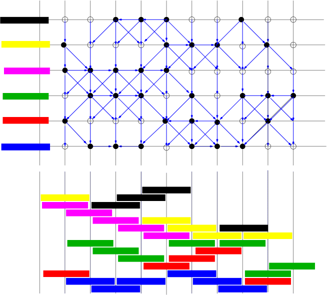
Figure 1: Top: A realization of the random graph ${\cal G}(p)$. Only the first 6 time-layers are represented. A black node at $(i,n)$ represents the arrival of a RACS of type $i$ at time $n$. Bottom: the associated the heap of RACS, with a visualization of the height $H_{n}^{i}$ of each RACS.

5.1.6 Exact Evolution Equations for the Model with Service

The system with service can be described as follows: there is an infinite number of servers, each of which serves with a unit rate. The servers are located at points $1/2+i$, $-\infty<i<\infty$. For each $i$, RACS $(i,n)$ (or customer $(i,n)$) is a customer of “type” $i$ that arrives with probability $p$ at time $n$ and needs one unit of time for simultaneous service from two servers located at points $i-1/2$ and $i+1/2$. So, at most one customer of each type arrives at each integer time instant. If customers of types $i$ and $i+1$ arrive at time $n$, then one makes a decision, that either $i$ arrives earlier or $i+1$ arrives earlier, at random with equal probabilities,

$${\mathbf{P}}(\mbox{customer}\ \ i\ \ \mbox{arrives earlier than customer}\ \ i+1)={\mathbf{P}}(e_{n}^{i,i+1}=l)=1/2.$$

Each server serves customers in the order of arrival. A customer leaves the system after the completion of its service. As before, we may assume that, for each $(i,n)$, customer $(i,n)$ arrives with probability $1$, but is “real”(“black”) with probability $p$ and “virtual”(“white”) with probability $1-p$.

Assume that the system is empty at time $0$ and that the first customers arrive at time $1$. Then, for any $n=1,2,\ldots$, the quantity $W_{n}^{i}:=\max(T_{n}^{i}-(n-1),0)$ is the residual amount of time (starting from time $n$) which is needed for the last real customer of type $i$ (among customers $(i,1),\ldots,(i,n)$) to receive the service (or equals zero if there is no real customers there).

Then these random variables satisfy the equations, for $n\geq 1,-\infty<i<\infty$,

$$W_{n+1}^{i} = (W_{n+1}^{i+1}+1){\bf I}(e_{n}^{i,i+1}=r,v_{n+1}^{i+1}=1,v_{n+1}^{i}=1)$$

$$\vee (W_{n+1}^{i-1}+1){\bf I}(e_{n}^{i-1,i}=l,v_{n+1}^{i-1}=1,v_{n+1}^{i}=1)$$

$$\vee ((W_{n}^{i}-1)^{+}+{\bf I}(v_{n+1}^{i}=1))$$

$$\vee ((W_{n}^{i-1}-1)^{+}+1){\bf I}(v_{n+1}^{i}=1)$$

$$\vee ((W_{n}^{i+1}-1)^{+}+1){\bf I}(v_{n+1}^{i}=1).$$

Since the heights are equal to 1 (and time intervals have length 1), the last two terms in the equation may be simplified, for instance, $((W_{n}^{i-1}-1)^{+}+1){\bf I}(v_{n+1}^{i}=1)$ may be replaced by $W_{n}^{i-1}{\bf I}(v_{n+1}^{i}=1).$

In the case of random heights $\{\sigma_{n}^{i}\}$, the random variables $\{W_{n}^{i}\}$ satisfy the recursions

$$W_{n+1}^{i} = (W_{n+1}^{i+1}+\sigma_{n+1}^{i}){\bf I}(e_{n}^{i,i+1}=r,v_{n+1}^{i+1}=1,v_{n+1}^{i}=1)$$

$$\vee (W_{n+1}^{i-1}+\sigma_{n+1}^{i}){\bf I}(e_{n}^{i-1,i}=l,v_{n+1}^{i-1}=1,v_{n+1}^{i}=1)$$

$$\vee ((W_{n}^{i}-1)^{+}+\sigma_{n+1}^{i}{\bf I}(v_{n+1}^{i}=1))$$

$$\vee ((W_{n}^{i-1}-1)^{+}+\sigma_{n+1}^{i}){\bf I}(v_{n+1}^{i}=1)$$

$$\vee ((W_{n}^{i+1}-1)^{+}+\sigma_{n+1}^{i}){\bf I}(v_{n+1}^{i}=1).$$

The following monotonicity property holds: for any $n$ and $i$,

$$W_{n+1}^{i}\circ\theta^{-n-1}\leq W_{n}^{i}\circ\theta^{-n}\quad\mbox{a.s.}$$

Let

$$p_{0}=\sup\{p\ :\ \Gamma(p)\leq 1\}.$$

Theorem 4

If $p<p_{0}$, then, for any $i$, random variables $W_{n}^{i}$ converge weakly to a proper limit. Moreover, there exists a stationary random vector $\{W^{i},-\infty<i<\infty\}$ such that, for any finite integers $i_{0}\leq 0\leq i_{1}$, the finite-dimensional random vectors

$$(W_{n}^{i_{0}},W_{n}^{i_{0}+1},\ldots,W_{n}^{i_{1}-1},W_{n}^{i_{1}})$$

converge weakly to the vector

$$(W^{i_{0}},W^{i_{0}+1},\ldots,W^{i_{1}-1}.W^{i_{1}})$$

Theorem 5

If $p<p_{0}$, then the random variables

$$\min\{i\geq 0\ :\ W^{i}=0\}\quad\mbox{and}\quad\max\{i\leq 0\ :\ W^{i}=0\}$$

are finite a.s.

6 Conclusion

We conclude with a few open questions. The first class of questions pertain to stochastic geometry [9]:

• How does the RACS exclusion process which is that of the RACS in service at time $t$ in steady state compare to other exclusion processes (e.g. Matérn, Gibbs)?

• Assuming that the system is stable, can the undirected graph of RACS present in the steady state regime percolate?

The second class of questions are classical in queueing theory and pertain to existence and properties of the stationary regime:

• In the stable case, does the stationary solution $\mathbb{W}_{\infty}^{0}$ always have a light tail? At the moment, we can show this under extra assumptions only. Notice that in spite of the fact that the Poisson hail model falls in the category of infinite dimensional max plus linear systems. Unfortunately, the techniques developed for analyzing the tails of the stationary regimes of finite dimensional max plus linear systems [3] cannot be applied here.

• In the stable case, does the Poisson hail equation (17) admit other stationary regimes than obtained from $\{\mathbb{W}_{\infty}^{x}\}_{x}$, the minimal stationary regime?

• For what other service disciplines still respecting the hard exclusion rule like e.g. priorities or first/best fit can one also construct a steady state?

7 Appendix

Proposition 1

For any pair $(X,Y)$ of random variables with light-tailed marginal distributions, there exists a coupling with another pair $(\xi,\eta)$ of i.i.d. random variables with a common light-tailed marginal distribution and such that

$$\max(X,Y)\leq\min(\xi,\eta)\quad\mbox{a.s}.$$

Proof. Let $F_{X}$ be the distribution function of $X$ and $F_{Y}$ the distribution function of $Y$. Let $C>0$ be such that ${\mathbf{E}}e^{CX}$ and ${\mathbf{E}}e^{CY}$ are finite. Let $\zeta=\max(0,X,Y)$. Since $e^{C\zeta}\leq 1+e^{CX}+e^{CY}$, $\zeta$ also has a light-tailed distribution, say $F$.

Let $\overline{F}(x)=1-F(x)$, $\overline{G}(x)=\overline{F}^{1/2}(x)$, and $G(x)=1-\overline{G}(x)$. Let $\xi$ and $\eta$ be i.i.d. with common distribution $G$. Then ${\mathbf{E}}^{c\xi}$ is finite, for any $c<C/2$.

Finally, a coupling of $X,Y,\xi$, and $\eta$ may be built as follows. Let $U_{1}$, $U_{2}$ be two i.i.d. random variable having uniform $(0,1)$ distribution. Then let $\xi=G^{-1}(U_{1})$, $\eta=G^{-1}(U_{2})$ and $\zeta=\min(\xi,\eta)$. Finally, define $X$ and $Y$ given $\max(X,Y)=\zeta$ and conditionally independent of $(\xi,\eta)$.

$\Box$

References

- [1] F. Baccelli and P. Brémaud, Elements of Queueing Theory, Springer Verlag, Applications of Mathematics, 2003.
- [2] F. Baccelli and S. Foss, “On the Saturation Rule for the Stability of Queues.” Journal of Applied Probability, 32(1995), 494–507.
- [3] F. Baccelli and S. Foss, “Moments and Tails in Monotone-Separable Stochastic Networks”, Annals of Applied Probability, 14 (2004), 621–650.
- [4] J.D. Biggins, “The first and last birth problems for a multitype age-dependent branching process”. Advances in Applied Probability, 8 (1976), 446–459.
- [5] B. Blaszczyszyn, C. Rau and V. Schmidt “Bounds for clump size characteristics in the Boolean model”. Adv. in Appl. Probab. 31, (1999), 910–928.
- [6] P. Hall, “On continuum percolation” Ann. Probab. 13, (1985), 1250–1266.
- [7] M. Loynes, “The stability of a queue with non-independentinter-arrival and service times”, Proceedings of the Cambridge Phil. Society, 58 (1962), 497–520.
- [8] D. Stoyan, Comparison Methods for Queues and other Stochastic Models, 1983, Wiley.
- [9] D. Stoyan, W.S. Kendall and J. Mecke, Stochastic Geometry and its Applications, second edition, 1995, Wiley.