Resonances Driven by a Neutrino Gyroscope and Collective Neutrino Oscillations in Supernovae

Abstract

We show that flavor evolution of a system of neutrinos with continuous energy spectra as in supernovae can be understood in terms of the response of individual neutrino flavor-isospins (NFIS’s) to the mean field. In the case of a system initially consisting of $\nu_{e}$ and $\bar{\nu}_{e}$ with the same energy spectrum but different number densities, the mean field is very well approximated by the total angular momentum of a neutrino gyroscope. Assuming that NFIS evolution is independent of the initial neutrino emission angle, the so-called single-angle approximation, we find that the evolution is governed by two types of resonances driven by precession and nutation of the gyroscope, respectively. The net flavor transformation crucially depends on the adiabaticity of evolution through these resonances. We show that the results for the system of two initial neutrino species can be extended to a system of four species with the initial number densities of $\nu_{e}$ and $\bar{\nu}_{e}$ significantly larger than those of $\nu_{x}$ and $\bar{\nu}_{x}$. Further, we find that when the dependence on the initial neutrino emission angle is taken into account in the multi-angle approximation, nutation of the mean field is quickly damped out and can be neglected. In contrast, precession-driven resonances still govern the evolution of NFIS’s with different energy and emission angles just as in the single-angle approximation. Our pedagogical and analytic study of collective neutrino oscillations in supernovae provides some insights into these seemingly complicated yet fascinating phenomena.

I Introduction

Experiments on solar, atmospheric, reactor, and accelerator neutrinos have found overwhelming evidence for neutrino flavor transformation via vacuum oscillations and the Mikheyev-Smirnov-Wolfenstein (MSW) effect (see Nakamura et al. (2010) (Particle Data Group) and references therein). The parameters governing these phenomena have largely been determined except for the neutrino mass hierarchy, the vacuum mixing angle $\theta_{13}$, and the CP-violation phase. For supernova neutrinos, in addition to the MSW effect induced by neutrino forward scattering on electrons in matter Wolfenstein (1978); Mikheyev and Smirnov (1985), novel phenomena of flavor transformation can occur (see Duan et al. (2010) and references therein) due to neutrino forward scattering on other neutrinos Fuller et al. (1987); Pantaleone (1992); Sigl and Raffelt (1993). This is because near the proto-neutron star produced in a supernova, the number density of neutrinos can exceed that of electrons. The dominance of neutrino-neutrino over neutrino-electron forward scattering couples flavor evolution of neutrinos that have different energy and travel on different trajectories, thereby giving rise to new phenomena. Assuming no CP-violation in the neutrino sector, Balantekin and Y$\rm{\ddot{u}}$ksel (2005); Fuller and Qian (2006); Duan et al. (2006a) first showed that collective oscillations of supernova neutrinos can occur for the vacuum-mass-squared difference $\delta m_{13}^{2}$ relevant for atmospheric neutrino oscillations. This collective flavor transformation can be treated effectively as $2\times 2$ mixing between $\nu_{e}$ and $\nu_{x}$ ($\bar{\nu}_{e}$ and $\bar{\nu}_{x}$), where $\nu_{x}$ ($\bar{\nu}_{x}$) is a superposition of $\nu_{\mu}$ and $\nu_{\tau}$ ($\bar{\nu}_{\mu}$ and $\bar{\nu}_{\tau}$), because $\nu_{\mu}$ and $\nu_{\tau}$ ($\bar{\nu}_{\mu}$ and $\bar{\nu}_{\tau}$) have identical emission characteristics and interactions in supernovae.

Subsequent to the study in Duan et al. (2006a), a number of authors have investigated collective oscillations of supernova neutrinos (see Duan et al. (2010) for a review). The most prominent feature of collective oscillations is the stepwise swap of the $\nu_{e}$ and $\nu_{x}$ energy spectra at some characteristic “split” energy Duan et al. (2006b); Raffelt and Smirnov (2007a). As this spectral swap for supernova neutrinos depends on the neutrino mass hierarchy (i.e., the sign of $\delta m_{13}^{2}$) and $\theta_{13}$, neutrino signals from a Galactic supernova can potentially provide a sensitive probe of both these unknown parameters.

Recently, it was found that spectral swaps for supernova neutrinos can occur at more than one energy Fogli et al. (2007); Dasgupta et al. (2009); Mirizzi and Tom$\rm{\grave{a}}$s (2010). Specifically, using supernova neutrino emission parameters with initial number densities of $\nu_{e}$ and $\bar{\nu}_{e}$ significantly larger than those of $\nu_{x}$ and $\bar{\nu}_{x}$, Fogli et al. (2007) found that for an inverted mass hierarchy (IH, the lightest mass eigenstate being dominantly $\nu_{x}$), an additional swap occurs in the spectra of $\bar{\nu}_{e}$ and $\bar{\nu}_{x}$ at a rather low energy. In contrast, using very different parameters with initial number densities of $\nu_{x}$ and $\bar{\nu}_{x}$ significantly larger than those of $\nu_{e}$ and $\bar{\nu}_{e}$, Dasgupta et al. (2009) and Mirizzi and Tom$\rm{\grave{a}}$s (2010) showed that spectral swaps occur at more than one energy for both IH and normal mass hierarchy (NH, the heaviest mass eigenstate being dominantly $\nu_{x}$).

In this paper we focus on the occurrence of spectral swaps for the case where the initial number densities of $\nu_{e}$ and $\bar{\nu}_{e}$ are significantly larger than those of $\nu_{x}$ and $\bar{\nu}_{x}$. As a concrete example, we assume that neutrinos are emitted in one of the flavor eigenstates $\nu_{a}$ (representing any one of $\nu_{e}$, $\nu_{x}$, $\bar{\nu}_{e}$, and $\bar{\nu}_{x}$) from a sharp neutrino sphere of radius $R_{\nu}=10$ km with a normalized spectrum of the form

$$f_{\nu_{a}}(E)=\frac{128}{3}\frac{E^{3}}{\langle E_{\nu_{a}}\rangle^{4}}\exp(-4E/\langle E_{\nu_{a}}\rangle),$$ (1)

where $\langle E_{\nu_{a}}\rangle$ is the average energy. We take $\langle E_{\nu_{e}}\rangle=10$ MeV, $\langle E_{\bar{\nu}_{e}}\rangle=15$ MeV, and $\langle E_{\nu_{x}}\rangle=\langle E_{\bar{\nu}_{x}}\rangle=24$ MeV. We further take the neutrino luminosity to be $L_{\nu_{a}}=10^{51}$ erg s^-1 for each species so that the initial number densities of $\nu_{e}$, $\bar{\nu}_{e}$, $\nu_{x}$, and $\bar{\nu}_{x}$ are in ratios of $2.4:1.6:1:1$.

We define $\delta m^{2}\equiv|\delta m^{2}_{13}|>0$ and $\theta_{\rm v}$ to be the parameters for vacuum mixing between $\nu_{e}$ and $\nu_{x}$ ($\bar{\nu}_{e}$ and $\bar{\nu}_{x}$), where $0<\theta_{\rm v}<\pi/4$ or $\pi/4<\theta_{\rm v}<\pi/2$ corresponds to the NH or IH, respectively. In accordance with the experimental limits on $\theta_{13}$, we take $\theta_{\rm v}\ll 1$ (NH) or $\tilde{\theta}_{\rm v}\equiv\pi/2-\theta_{\rm v}\ll 1$ (IH). Following the definition of Duan et al. (2006a), we represent each neutrino by a neutrino flavor isospin (NFIS) $\mathbf{s}$ of magnitude $1/2$ in a three-dimensional flavor space. In particular,

$$\mathbf{s}=\begin{cases}\mathbf{\hat{e}}_{z}^{\rm f}/2,&\mbox{for $\nu_{e}$ or $\bar{\nu}_{x}$},\\ -\mathbf{\hat{e}}_{z}^{\rm f}/2,&\mbox{for $\nu_{x}$ or $\bar{\nu}_{e}$},\end{cases}$$ (2)

where $\mathbf{\hat{e}}_{z}^{\rm f}$ is the unit vector in the $z$-direction of the flavor space. It is convenient to use

$$\omega\equiv\begin{cases}\delta m^{2}/2E,&\mbox{for $\nu_{e}$ and $\nu_{x}$},\\ -\delta m^{2}/2E,&\mbox{for $\bar{\nu}_{e}$ and $\bar{\nu}_{x}$},\end{cases}$$ (3)

to label the NFIS of an initial $\nu_{a}$ with energy $E$ as $\mathbf{s}_{\omega}$.

We follow the flavor evolution of neutrinos in the above example from the neutrino sphere to a radius $r=250$ km, where oscillations have effectively ceased. We focus on the IH with $\delta m^{2}=3\times 10^{-3}$ eV² and assume $\tilde{\theta}_{\rm v}=10^{-5}$ in view of matter suppression of mixing, but otherwise ignore the matter above the neutrino sphere. We further assume that the flavor evolution of a $\nu_{a}$ emitted in a non-radial direction is identical to that of another $\nu_{a}$ with the same energy but emitted radially. This is the so-called “single-angle” approximation. The effective total number density at radius $r>R_{\nu}$ for neutrinos emitted initially as $\nu_{a}$ is taken to be

$$n_{\nu_{a}}(r)=\frac{L_{\nu_{a}}}{4\pi R_{\nu}^{2}\langle E_{\nu_{a}}\rangle}\left[1-\sqrt{1-(R_{\nu}/r)^{2}}\right]^{2}.$$ (4)

The evolution of the NFIS $\mathbf{s}_{\omega}$ with time $t$, or equivalently, with radius $r$ is governed by

$$\frac{d}{dt}\mathbf{s}_{\omega}=\frac{d}{dr}\mathbf{s}_{\omega}=\mathbf{s}_{\omega}\times\left[\omega\mathbf{H}_{\rm v}-2\sqrt{2}G_{F}\sum_{a}n_{\nu_{a}}(r)\int_{0}^{\infty}\mathbf{s}_{\omega^{\prime}}f_{\nu_{a}}(E)dE\right],$$ (5)

where $\mathbf{H}_{\rm v}\equiv-\sin 2\theta_{\rm v}\mathbf{\hat{e}}_{x}^{\rm f}+\cos 2\theta_{\rm v}\mathbf{\hat{e}}_{z}^{\rm f}=-\sin 2\tilde{\theta}_{\rm v}\mathbf{\hat{e}}_{x}^{\rm f}-\cos 2\tilde{\theta}_{\rm v}\mathbf{\hat{e}}_{z}^{\rm f}$, $G_{F}$ is the Fermi constant, and $\omega^{\prime}$ runs over all NFIS’s as summation over $a$ and integration over $E$ are performed. For convenience, we adopt the natural units, where the Planck constant $\hbar$ and the speed of light $c$ are set to unity, in writing expressions and equations throughout the paper.

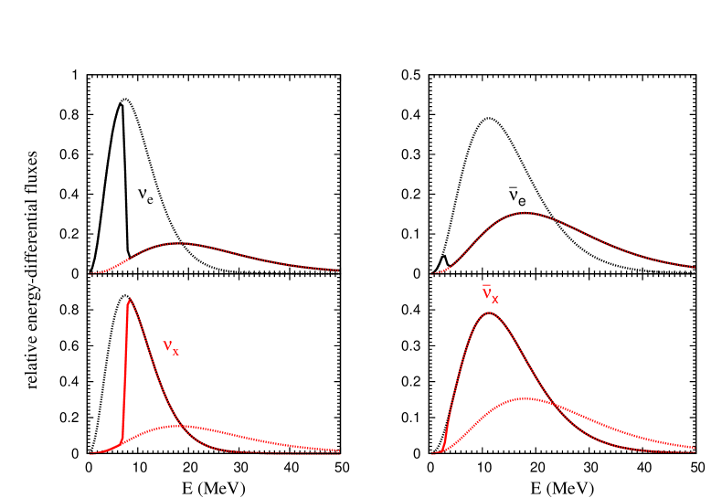
Figure 1: An example of stepwise spectral swaps for the IH and for the case where the initial number densities of $\nu_{e}$ and $\bar{\nu}_{e}$ are significantly larger than those of $\nu_{x}$ and $\bar{\nu}_{x}$. The neutrino flux spectra at the neutrino sphere (dashed curves) and at $r=250$ km (solid curves) are shown. The dashed curves with larger maxima are for the initial $\nu_{e}$ and $\bar{\nu}_{e}$ while those with lower maxima are for the initial $\nu_{x}$ and $\bar{\nu}_{x}$. It can be seen that the $\nu_{e}$ and $\nu_{x}$ spectra are swapped for $E\gtrsim 7.6$ MeV and the $\bar{\nu}_{e}$ and $\bar{\nu}_{x}$ spectra are swapped for $E\gtrsim 3.1$ MeV.

Figure 1 compares the neutrino flux spectra at the neutrino sphere (dashed curves) and at $r=250$ km (solid curves). The vertical scale measures the relative energy-differential fluxes, which are $\propto L_{\nu_{a}}f_{\nu_{a}}(E)/\langle E_{\nu_{a}}\rangle$ at the neutrino sphere. It can be seen that the $\nu_{e}$ and $\nu_{x}$ spectra are swapped for $E\gtrsim 7.6$ MeV and the $\bar{\nu}_{e}$ and $\bar{\nu}_{x}$ spectra are swapped for $E\gtrsim 3.1$ MeV. To highlight these spectral changes, we define a “swap factor”

$$f_{S}(\omega,t)\equiv s^{\rm f}_{\omega,z}(t)/s^{\rm f}_{\omega,z}(0),$$ (6)

where $s^{\rm f}_{\omega,z}(t)\equiv\mathbf{s}_{\omega}(t)\cdot{\mathbf{\hat{e}}}^{\rm f}_{z}$. The value of $f_{S}(\omega,t)=1$ or $-1$ corresponds to complete survival or conversion of the initial $\nu_{a}$, respectively. The swap factor $f_{S}(\omega,t)$ at $r=250$ km for the above example is shown as a function of $2\omega/\delta m^{2}$ in Fig. 2.

Figure 2: The swap factor $f_{S}(\omega,t)$ at $r=250$ km as a function of $2\omega/\delta m^{2}$ for the example shown in Fig. 1. Note that the negative range of the horizontal axis corresponds to $\bar{\nu}_{e}$ and $\bar{\nu}_{x}$ while the positive range corresponds to $\nu_{e}$ and $\nu_{x}$.

The main goal of this paper is to explain how spectral swaps occur in the above example. Our approach is pedagogical. In Sec. II we consider the net effect of all the NFIS’s in the above example as a “mean field” to which an individual $\mathbf{s}_{\omega}$ responds. We show that the evolution of this mean field can be well described by the motion of a “neutrino gyroscope” over a wide range of neutrino densities. In Sec. III we discuss in detail the precession and nutation of the neutrino gyroscope. In Sec. IV we show that the response of an NFIS to the mean field is characterized by two types of resonances driven by the precession and nutation of the neutrino gyroscope, respectively. These resonances and the adiabaticity of evolution through them give rise to the stepwise spectral swaps. In Sec. V, we relax the single-angle approximation and discuss the evolution of NFIS’s along different trajectories in realistic supernova environments. We show that the trajectory-dependent evolution strongly suppresses nutation of the neutrino gyroscope. Consequently, the spectral swaps in this case are determined by precession-driven resonances only. We summarize our results and give conclusions in Sec. VI.

II Mean Field of NFIS’s and Neutrino Gyroscope

The NFIS for an initial $\nu_{e}$ and that for an initial $\nu_{x}$ with the same energy (or $\omega$) are equal in magnitude but opposite in direction [see Eq. (2)]. It can be seen from Eq. (5) that these two NFIS’s remain equal in magnitude but opposite in direction during their subsequent evolution. The same is also true of the NFIS’s for an initial $\bar{\nu}_{e}$ and an initial $\bar{\nu}_{x}$ with the same energy. Hereafter, $\mathbf{s}_{\omega}$ for $\omega>0$ or $\omega<0$ refers to the NFIS for an initial $\nu_{e}$ or $\bar{\nu}_{e}$, respectively. Then Eq. (5) can be rewritten as

$$\frac{d}{dr}\mathbf{s}_{\omega}=\mathbf{s}_{\omega}\times\left[\omega\mathbf{H}_{\rm v}-\mu(r)\int_{-\infty}^{\infty}g(\omega^{\prime})\mathbf{s}_{\omega^{\prime}}d\omega^{\prime}\right],$$ (7)

where $\mu(r)\equiv 2\sqrt{2}G_{F}n_{\nu_{e}}(r)$. In the above equation,

$$g(\omega)=\frac{\delta m^{2}}{2\omega^{2}}\times\begin{cases}c_{e}f_{\nu_{e}}(E_{\omega})-c_{x}f_{\nu_{x}}(E_{\omega}),&\mbox{for $\omega>0$},\\ c_{\bar{e}}f_{\bar{\nu}_{e}}(E_{\omega})-c_{\bar{x}}f_{\bar{\nu}_{x}}(E_{\omega}),&\mbox{for $\omega<0$},\end{cases}$$ (8)

where $c_{a}=n_{\nu_{a}}(R_{\nu})/n_{\nu_{e}}(R_{\nu})=\langle E_{\nu_{a}}\rangle/\langle E_{\nu_{e}}\rangle$ and $E_{\omega}=\delta m^{2}/2|\omega|$.

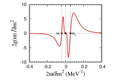
Figure 3: Example supernova neutrino spectrum shown in terms of $2g(\omega)/\delta m^{2}$ as a function of $2\omega/\delta m^{2}$. There are three spectral crossings (filled circles) at $\omega=\omega_{-}$, 0, and $\omega_{+}$, respectively, for which $g(\omega)=0$.

We define

$$\mathbf{S}\equiv\int_{-\infty}^{\infty}g(\omega)\mathbf{s}_{\omega}d\omega$$ (9)

and consider it as the mean field representing the net effect of all NFIS’s to which an individual $\mathbf{s}_{\omega}$ responds. Clearly, an exact description of the mean field requires solving Eq. (7) for all NFIS’s. However, we can give an approximate description based on the evolution of a small number of NFIS’s. To see this, we show $2g(\omega)/\delta m^{2}$ as a function of $2\omega/\delta m^{2}$ for our supernova example in Fig. 3. There are three “spectral crossings” Dasgupta et al. (2009) at $\omega=\omega_{-}$, 0, and $\omega_{+}$, respectively, for which $g(\omega)=0$. In each of the four spectral regions separated by these crossings, the magnitude of $g(\omega)$ is large only for a relatively narrow range of $\omega$.

We consider that the four spectral regions $(-\infty,\omega_{-})$, $(\omega_{-},0)$, $(0,\omega_{+})$, and $(\omega_{+},\infty)$ can be represented by four effective NFIS’s $\mathbf{s}_{\bar{e}}^{(0)}$, $\mathbf{s}_{\bar{x}}^{(0)}$, $\mathbf{s}_{x}^{(0)}$, and $\mathbf{s}_{e}^{(0)}$, respectively, which correspond to a $\bar{\nu}_{e}$, a $\bar{\nu}_{x}$, a $\nu_{x}$, and a $\nu_{e}$ at the neutrino sphere. We then approximate $\mathbf{S}$ by

$$\mathbf{S}^{(0)}=\alpha_{e}\mathbf{s}_{e}^{(0)}+\alpha_{x}\mathbf{s}_{x}^{(0)}+\alpha_{\bar{x}}\mathbf{s}_{\bar{x}}^{(0)}+\alpha_{\bar{e}}\mathbf{s}_{\bar{e}}^{(0)},$$ (10)

where the evolution of each $\mathbf{s}_{a}^{(0)}$ is governed by

$$\frac{d}{dr}{\mathbf{s}}_{a}^{(0)}=\mathbf{s}_{a}^{(0)}\times\left[\omega_{a}\mathbf{H}_{\rm v}-\mu(r)\mathbf{S}^{(0)}\right].$$ (11)

In the above equations,

$$\alpha_{e} =\int_{\omega_{+}}^{\infty}|g(\omega)|d\omega,$$ (12)

$$\omega_{e} =\frac{1}{\alpha_{e}}\int_{\omega_{+}}^{\infty}\omega|g(\omega)|d\omega,$$ (13)

and other quantities are defined similarly. For our supernova example, $\alpha_{e}=0.78$, $\alpha_{x}=0.20$, $\alpha_{\bar{x}}=0.10$, and $\alpha_{\bar{e}}=0.35$, while $2\omega_{a}/\delta m^{2}=0.15$, 0.032, $-0.027$, and $-0.11$ MeV^-1 for $\mathbf{s}_{e}^{(0)}$, $\mathbf{s}_{x}^{(0)}$, $\mathbf{s}_{\bar{x}}^{(0)}$, and $\mathbf{s}_{\bar{e}}^{(0)}$, respectively.

At the neutrino sphere, $\mathbf{S}=\mathbf{S}^{(0)}={\mathbf{\hat{e}}}^{\rm f}_{z}/6$. As can be shown from Eqs. (7) and (11), the components of $\mathbf{S}$ and $\mathbf{S}^{(0)}$ parallel to $\mathbf{H}_{\rm v}$ are conserved during the subsequent evolution. We numerically obtain their components perpendicular to $\mathbf{H}_{\rm v}$, $S_{\perp}$ (solid curve) and $S^{(0)}_{\perp}$ (dashed curve), and show these as functions of $\mu(r)/\omega_{e}$ in Fig. 4. It can be seen that $S^{(0)}_{\perp}$ closely tracks $S_{\perp}$ for $\mu(r)/\omega_{e}\gtrsim 20$ but large deviations occur for $\mu(r)/\omega_{e}<10$. In particular, $S^{(0)}_{\perp}$ diverges from $S_{\perp}$ at $\mu(r)/\omega_{e}<4$. The above results can be understood by comparing $\mu(r)|\mathbf{S}|$ with the spread in $\omega$ for the spectrum shown in Fig. 3. For $\mu(r)/\omega_{e}\gtrsim 20$, $\mu(r)|\mathbf{S}|\gtrsim 3\omega_{e}$ exceeds the spread over the entire spectrum, which is $\sim 2\omega_{e}$. So all NFIS’s evolve collectively in this regime and the four effective NFIS’s included in $\mathbf{S}^{(0)}$ are sufficient to give a good description of $\mathbf{S}$. For $\mu(r)/\omega_{e}\sim 10$, $\mu(r)|\mathbf{S}|\sim\omega_{e}$ approaches $\Delta\omega_{e}=0.66\omega_{e}$, which is the spread in the spectral region $(\omega_{+},\infty)$ calculated from

$$\Delta\omega_{e}=\frac{1}{\alpha_{e}}\left[\int_{\omega_{+}}^{\infty}(\omega-\omega_{e})^{2}|g(\omega)|d\omega\right]^{1/2}.$$ (14)

Consequently, for $\mu(r)/\omega_{e}<10$, the NFIS’s in the above spectral region are no longer well represented by $\mathbf{s}_{e}^{(0)}$ and large differences between $S^{(0)}_{\perp}$ and $S_{\perp}$ occur. Eventually, none of the effective NFIS’s can represent their respective spectral regions and $S^{(0)}_{\perp}$ diverges from $S_{\perp}$.

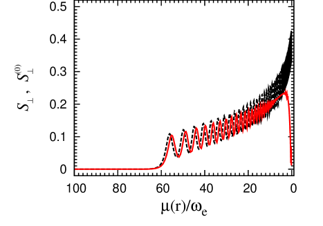
Figure 4: Comparison of $S_{\perp}$ (solid curve) and $S^{(0)}_{\perp}$ (dashed curve) as functions of $\mu(r)/\omega_{e}$ for the supernova example.

In a formal approach, we can use $\mathbf{S}^{(0)}$ as the zeroth order approximation for $\mathbf{S}$ to solve Eq. (7) for the evolution of $\mathbf{s}_{\omega}$, and use the results to obtain a better approximation for $\mathbf{S}$ from Eq. (9). This procedure may be repeated until successive approximations for $\mathbf{S}$ converge. While this approach does not save numerical efforts compared with solving Eq. (7) directly, it motivates an analytic study based on the zeroth order mean field $\mathbf{S}^{(0)}$, especially when $\mathbf{S}^{(0)}$ can be understood with simple models. We carry out such a study in the rest of the paper. We first consider a simpler case and then apply the results from this case to discuss the supernova example in Sec. V.

II.1 System Initially Consisting of $\nu_{e}$ and $\bar{\nu}_{e}$ Only

In our supernova example, the initial number densities of $\nu_{e}$ and $\bar{\nu}_{e}$ are significantly larger than those of $\nu_{x}$ and $\bar{\nu}_{x}$. To facilitate an analytic study, we consider a simpler system initially consisting of $\nu_{e}$ and $\bar{\nu}_{e}$ only. We take normalized emission spectra of the form in Eq. (1) with $\langle E_{\nu_{e}}\rangle=\langle E_{\bar{\nu}_{e}}\rangle=12$ MeV and luminosities $L_{\nu_{e}}=1.2\times 10^{51}$ and $L_{\bar{\nu}_{e}}=0.8\times 10^{51}$ erg s^-1 so that the initial number densities of $\nu_{e}$ and $\bar{\nu}_{e}$ are the same as those in the supernova example. In this case, the effective neutrino spectrum $g(\omega)$ reduces to

$$h(\omega)=\frac{\delta m^{2}}{2\omega^{2}}\times\begin{cases}f_{\nu_{e}}(E_{\omega}),&\mbox{for $\omega>0$},\\ \alpha f_{\bar{\nu}_{e}}(E_{\omega}),&\mbox{for $\omega<0$},\end{cases}$$ (15)

where $\alpha=n_{\bar{\nu}_{e}}(R_{\nu})/n_{\nu_{e}}(R_{\nu})=2/3$.

We consider that the zeroth order approximation for the mean field $\mathbf{S}=\int_{-\infty}^{\infty}h(\omega)\mathbf{s}_{\omega}d\omega$ is given by

$$\mathbf{S}^{(0)}\equiv\mathbf{s}_{1}^{(0)}+\alpha\mathbf{s}_{2}^{(0)},$$ (16)

where $\mathbf{s}_{1}^{(0)}$ and $\mathbf{s}_{2}^{(0)}$ are the NFIS’s for an initial $\nu_{e}$ and an initial $\bar{\nu}_{e}$ with

$$\omega_{1}=\int_{0}^{\infty}\omega h(\omega)d\omega,$$ (17a)

$$\omega_{2}=\frac{1}{\alpha}\int_{-\infty}^{0}\omega h(\omega)d\omega,$$ (17b)

respectively. Specifically, $\omega_{1}=-\omega_{2}\equiv\mu_{\rm v}$ and $2\mu_{\rm v}/\delta m^{2}=1/9$ MeV^-1. We show $S_{\perp}$ (solid curve) and $S^{(0)}_{\perp}$ (dashed curve) as functions of $\mu(r)/\mu_{\rm v}$ in Fig. 5. It can be seen that the comparison between $S_{\perp}$ and $S^{(0)}_{\perp}$ is very similar to that in the supernova example [note that the horizontal scales for Figs. 4 and 5 are related by $\mu(r)/\mu_{\rm v}=1.35\mu(r)/\omega_{e}$].

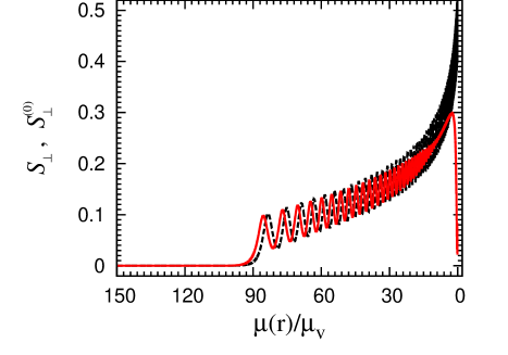
Figure 5: Comparison of $S_{\perp}$ (solid curve) and $S^{(0)}_{\perp}$ (dashed curve) as functions of $\mu(r)/\mu_{\rm v}$ for the system initially consisting of $\nu_{e}$ and $\bar{\nu}_{e}$ only.

The swap factor $f_{S}(\omega,t)$ at $r=250$ km for the system initially consisting of $\nu_{e}$ and $\bar{\nu}_{e}$ only is shown as the solid curve in Fig. 6. The swap factor $f_{S}^{(0)}(\omega,t)$ calculated from

$$\frac{d}{dr}{\mathbf{s}}_{\omega}=\mathbf{s}_{\omega}\times\left[\omega\mathbf{H}_{\rm v}-\mu(r)\mathbf{S}^{(0)}\right],$$ (18)

which uses $\mathbf{S}^{(0)}$ to approximate $\mathbf{S}$, is shown as the dashed curve. It can be seen that just as in the supernova example, $f_{S}(\omega,t)$ and $f_{S}^{(0)}(\omega,t)$ have two characteristic split energies, one in the region of $\omega>0$ and the other in the region of $\omega<0$. Although $f_{S}^{(0)}(\omega,t)$ has a different split energy from that of $f_{S}(\omega,t)$ in the region of $\omega<0$, they have the same qualitative behavior, especially the same split energy in the region of $\omega>0$. Our goal is to understand the behavior of $f_{S}^{(0)}(\omega,t)$ analytically.

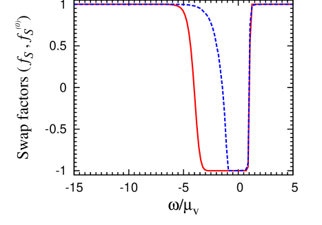
Figure 6: Comparison of the swap factors $f_{S}(\omega,t)$ (solid curve) and $f_{S}^{(0)}(\omega,t)$ (dashed curve) at $r=250$ km for the system initially consisting of $\nu_{e}$ and $\bar{\nu}_{e}$ only.

II.2 Neutrino Gyroscope as the Approximate Mean Field

For the system initially consisting of $\nu_{e}$ and $\bar{\nu}_{e}$ only, the evolution of $\mathbf{s}_{1}^{(0)}$ and $\mathbf{s}_{2}^{(0)}$ is governed by

$$\frac{d}{dr}{\mathbf{s}}_{1}^{(0)} =\mathbf{s}_{1}^{(0)}\times\left[\mu_{\rm v}\mathbf{H}_{\rm v}-\mu(r)\mathbf{S}^{(0)}\right],$$ (19a)

$$\frac{d}{dr}{\mathbf{s}}_{2}^{(0)} =\mathbf{s}_{2}^{(0)}\times\left[-\mu_{\rm v}\mathbf{H}_{\rm v}-\mu(r)\mathbf{S}^{(0)}\right].$$ (19b)

For convenience, we will drop the superscript “(0)” but otherwise use the symbols in the same meaning as in the above equations. It is useful to consider the time evolution of $\mathbf{s}_{1}$ and $\mathbf{s}_{2}$ at a constant $\mu$ governed by

$$\mathbf{\dot{s}}_{1} \equiv\frac{d}{dt}\mathbf{s}_{1}=\mathbf{s}_{1}\times(\mu_{\rm v}\mathbf{H}_{\rm v}-\mu\mathbf{S}),$$ (20a)

$$\mathbf{\dot{s}}_{2} \equiv\frac{d}{dt}\mathbf{s}_{2}=\mathbf{s}_{2}\times(-\mu_{\rm v}\mathbf{H}_{\rm v}-\mu\mathbf{S}).$$ (20b)

As discussed in Hannestad et al. (2006); Duan et al. (2007) and repeated below, the system governed by the above equations is mathematically equivalent to a gyroscope in a uniform gravitational field.

From Eqs. (20a) and (20b) it is straightforward to show that

$$\mathbf{\dot{Q}} =\mu\mathbf{S}\times\mathbf{Q},$$ (21a)

$$\mathbf{\dot{S}} =\mu_{\rm v}\mathbf{Q}\times\mathbf{H}_{\rm v},$$ (21b)

where

$$\mathbf{Q}=\mathbf{s}_{1}-\alpha\mathbf{s}_{2}+\frac{\mu_{\rm v}}{\mu}\mathbf{H}_{\rm v}.$$ (22)

From Eq. (21a) it can be shown that $Q\equiv|\mathbf{Q}|$ is conserved. With the definition of a unit vector $\mathbf{\hat{r}}\equiv\mathbf{Q}/Q$, Eqs. (21a) and (21b) can be rewritten as

$$\mathbf{S} =\frac{1}{\mu}\mathbf{\hat{r}}\times\mathbf{\dot{\hat{r}}}+\sigma\mathbf{\hat{r}},$$ (23a)

$$\mathbf{\dot{S}} =\frac{1}{\mu}\mathbf{\hat{r}}\times\mathbf{g},$$ (23b)

where $\sigma\equiv\mathbf{S}\cdot\hat{\mathbf{r}}$ and $\mathbf{g}\equiv\mu\mu_{\rm v}Q\mathbf{H}_{\rm v}$. The above equations describe the motion of a gyroscope in a uniform gravitational field with an acceleration of gravity $\mathbf{g}$ (see Fig. 7a). The gyroscope has a spinning point particle of mass $1/\mu$ attached to the tip of a massless rod of unit length. The spin of the gyroscope is along the direction $\mathbf{\hat{r}}$ of the rod and it can be shown from Eqs. (21a) and (21b) that the magnitude $\sigma$ of the spin is conserved. As can be seen from Eq. (23b), the component of the total angular momentum $\mathbf{S}$ parallel to $\mathbf{H}_{\rm v}$ is also conserved.

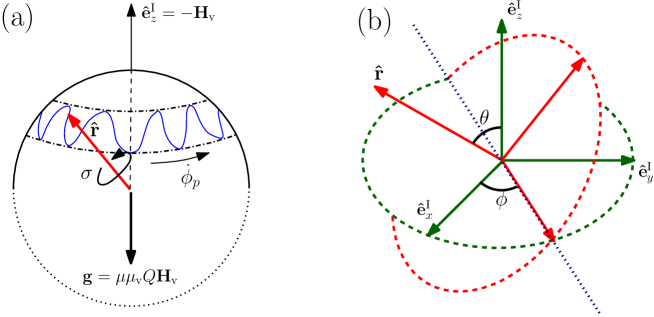
Figure 7: Illustration of (a) the neutrino gyroscope and (b) the Euler angles $\theta$ and $\phi$ used to describe its motion in Frame I. The gyroscope has a spinning point particle of mass $1/\mu$ attached to the tip of a massless rod of unit length. The spin is along the direction $\mathbf{\hat{r}}$ of the rod and has a magnitude $\sigma$. The gyroscope is in a uniform gravitational field with an acceleration of gravity $\mathbf{g}$. The wiggly curve on the spherical surface crudely indicates the trajectory of the tip of $\mathbf{\hat{r}}$ as the gyroscope executes precession (change in $\phi$, arrow labeled by $\dot{\phi}_{p}$) and nutation (change in $\theta$) at a constant $\mu$.

If $\mu$ varies smoothly with time, the neutrino gyroscope described above evolves through a series of configurations corresponding to a continuous range of $\mu$. The motion of this gyroscope provides a well-studied mechanical analog to the evolution of the approximate mean field.

III Precession and Nutation of The Neutrino Gyroscope

We specify the unit vector $\mathbf{\hat{r}}$ of the neutrino gyroscope by two of the Euler angles, $\theta$ and $\phi$, in Frame I:

$$\mathbf{\hat{r}}=\sin\theta\sin\phi\,\mathbf{\hat{e}}_{x}^{\rm I}-\sin\theta\cos\phi\,\mathbf{\hat{e}}_{y}^{\rm I}+\cos\theta\,\mathbf{\hat{e}}_{z}^{\rm I},$$ (24)

where $\mathbf{\hat{e}}_{x}^{\rm I}$, $\mathbf{\hat{e}}_{y}^{\rm I}$, and $\mathbf{\hat{e}}_{z}^{\rm I}$ are the unit vectors associated with the three axes of Frame I and $\mathbf{\hat{e}}_{z}^{\rm I}=-\mathbf{H}_{\rm v}$ (see Fig. 7). We focus on the IH with $\tilde{\theta}_{\rm v}\ll 1$, for which $\mathbf{H}_{\rm v}=-\sin 2\tilde{\theta}_{\rm v}\mathbf{\hat{e}}_{x}^{\rm f}-\cos 2\tilde{\theta}_{\rm v}\mathbf{\hat{e}}_{z}^{\rm f}\approx-{\mathbf{\hat{e}}}^{\rm f}_{z}$. Thus, $\mathbf{\hat{e}}_{z}^{\rm I}\approx{\mathbf{\hat{e}}}^{\rm f}_{z}$ is the upward direction and $\mathbf{g}$ (in the same direction as $\mathbf{H}_{\rm v}$) points downward (see Fig. 7a). When the neutrino gyroscope starts at $\mu\gg\mu_{\rm v}$, $\mathbf{Q}\approx\mathbf{s}_{1}-\alpha\mathbf{s}_{2}$ points in the direction of ${\mathbf{\hat{e}}}^{\rm f}_{z}$, i.e., it is in the upright position. This initial configuration can give rise to interesting subsequent evolution.

III.1 Motion of the Neutrino Gyroscope at Constant $\mu$

We first discuss motion of the neutrino gyroscope at constant $\mu$. Using Eq. (23a), we can express $\mathbf{S}$ in terms of $\theta$ and $\phi$ as

$$S_{x} =\frac{1}{\mu}(\dot{\theta}\cos\phi-\dot{\phi}\sin\theta\cos\theta\sin\phi)+\sigma\sin\theta\sin\phi,$$ (25a)

$$S_{y} =\frac{1}{\mu}(\dot{\theta}\sin\phi+\dot{\phi}\sin\theta\cos\theta\cos\phi)-\sigma\sin\theta\cos\phi,$$ (25b)

$$S_{z} =\frac{1}{\mu}\dot{\phi}\sin^{2}\theta+\sigma\cos\theta=\frac{1-\alpha}{2}\cos 2\tilde{\theta}_{\rm v},$$ (25c)

where we have used conservation of $S_{z}$ in the exact form (i.e., no approximation made for $\tilde{\theta}_{\rm v}\ll 1$) in the last equation. In addition to $\sigma$ and $S_{z}$, the third conserved quantity of the gyroscope is its total energy:

$$E_{\rm gyro} =\frac{\mu}{2}\mathbf{S}^{2}-\frac{1}{\mu}\mathbf{\hat{r}}\cdot\mathbf{g},$$ (26a)

$$=\frac{1}{2\mu}\left(\dot{\theta}^{2}+\dot{\phi}^{2}\sin^{2}\theta\right)+\frac{\mu}{2}\sigma^{2}+\mu_{\rm v}Q\cos\theta.$$ (26b)

Conservation of $E_{\rm gyro}$ can be shown using Eqs. (23a) and (23b). We can also derive an explicit equation of motion from Eq. (23b):

$$\ddot{\theta}-\dot{\phi}(\dot{\phi}\cos\theta-\mu\sigma)\sin\theta=\mu\mu_{\rm v}Q\sin\theta.$$ (27)

In general, both $\theta$ and $\phi$ of a gyroscope evolve with time, and the corresponding motion (see Fig. 7) is referred to as nutation ($\theta$) and precession ($\phi$). For the neutrino gyroscope, conservation of $\sigma$, $S_{z}$, $E_{\rm gyro}$ can be combined to give a conserved effective energy associated with nutation only:

$$E_{\theta}=E_{\rm gyro}-\frac{\mu}{2}\sigma^{2}=\frac{\dot{\theta}^{2}}{2\mu}+V_{\rm eff}(\theta),$$ (28)

where

$$V_{\rm eff}(\theta)=\frac{\mu}{2}\frac{(S_{z}-\sigma\cos\theta)^{2}}{\sin^{2}\theta}+\mu_{\rm v}Q\cos\theta.$$ (29)

As shown in Sec. III.2, nutation of the neutrino gyroscope mostly occurs around the minimum of the effective potential $V_{\rm eff}(\theta)$. This potential minimum corresponds to $\theta=\theta_{p}$, for which

$$\left.\frac{dV_{\rm eff}}{d\theta}\right|_{\theta_{p}} =\mu\frac{(S_{z}-\sigma\cos\theta_{p})(\sigma-S_{z}\cos\theta_{p})}{\sin^{3}\theta_{p}}-\mu_{\rm v}Q\sin\theta_{p}=0,$$ (30a)

$$\mu\left.\frac{d^{2}V_{\rm eff}}{d\theta^{2}}\right|_{\theta_{p}} =\dot{\phi}_{p}^{2}\sin^{2}\theta_{p}+\left(2\dot{\phi}_{p}\cos\theta_{p}-\mu\sigma\right)^{2}\equiv\omega_{n}^{2}>0.$$ (30b)

In Eq. (30b), $\dot{\phi}_{p}$ is the instantaneous precession frequency at the potential minimum and can be obtained from Eq. (25c) after $\theta_{p}$ is solved from Eq. (30a). Note that Eq. (30a) is the same as

$$\dot{\phi}_{p}(\dot{\phi}_{p}\cos\theta_{p}-\mu\sigma)+\mu\mu_{\rm v}Q=0,$$ (31)

which can also be obtained by setting $\ddot{\theta}=0$ and $\dot{\phi}=\dot{\phi}_{p}$ in Eq. (27). In other words, the minimum $V_{\rm eff}$ corresponds to the maximum $\dot{\theta}$ [due to conservation of $E_{\theta}$, see Eq. (28)], and hence $\ddot{\theta}=0$.

To the leading order, nutation can be approximated as oscillations of $\theta$ around $\theta_{p}$ in response to the potential

$$V_{\rm eff}(\theta)\approx V_{\rm eff}(\theta_{p})+\frac{\omega_{n}^{2}}{2\mu}(\theta-\theta_{p})^{2}.$$ (32)

In this approximation, the evolution of $\theta$ can be described by

$$\theta \approx\theta_{p}-\eta\cos(\omega_{n}t+\beta),$$ (33a)

$$\dot{\theta} \approx\eta\omega_{n}\sin(\omega_{n}t+\beta),$$ (33b)

where $\eta$ is the amplitude of oscillation (or nutation) and $\beta$ is a constant phase. The values of $\eta$ and $\beta$ are determined by the initial values of $\theta$ and $\dot{\theta}$ at $t=0$. Using Eq. (25c) to relate $\dot{\phi}$ at $\theta$ to $\dot{\phi}_{p}$ at $\theta_{p}$, we obtain to the first order in $\eta$,

$$\dot{\phi} \approx\dot{\phi}_{p}-\eta\left[\frac{\mu\sigma-2\dot{\phi}_{p}\cos\theta_{p}}{\sin\theta_{p}}\right]\cos(\omega_{n}t+\beta),$$ (34a)

$$\phi \approx\gamma+\dot{\phi}_{p}t-\eta\left[\frac{\mu\sigma-2\dot{\phi}_{p}\cos\theta_{p}}{\omega_{n}\sin\theta_{p}}\right]\sin(\omega_{n}t+\beta),$$ (34b)

where $\gamma$ is a constant determined by the initial value of $\phi$ at $t=0$.

From Eqs. (25a)–(25c) and (33a)–(34b) we obtain

$$S_{x}+iS_{y} \approx i\left\{\left(\frac{\dot{\phi}_{p}}{\mu}\cos\theta_{p}-\sigma\right)\sin\theta_{p}+\frac{\eta}{2}\frac{\dot{\phi}_{p}}{\mu}\left[\left(1-\frac{2\dot{\phi}_{p}-\mu S_{z}}{\omega_{n}}\right)e^{i(\omega_{n}t+\beta)}\right.\right.$$

$$+\left.\left.\left(1+\frac{2\dot{\phi}_{p}-\mu S_{z}}{\omega_{n}}\right)e^{-i(\omega_{n}t+\beta)}\right]\right\}e^{i(\dot{\phi}_{p}t+\gamma)},$$ (35)

which is accurate to the first order in $\eta$. The above equation shows that to the leading order, the angular momentum $\mathbf{S}$ can be described by three precessing vectors with different amplitudes and different precession frequencies, which are $\dot{\phi}_{p}$, $\dot{\phi}_{p}+\omega_{n}$, and $\dot{\phi}_{p}-\omega_{n}$, respectively. This leading-order expression of $\mathbf{S}$ provides a very useful analytic description of the motion of the neutrino gyroscope. Without loss of generality, hereafter we set the phase constants $\beta=\gamma=0$ in Eq. (35).

III.2 Motion of the Neutrino Gyroscope for Slowly Decreasing $\mu$

We now extend the discussion in Sec. III.1 for a constant $\mu$ to the case where $\mu(t)$ slowly decreases with time from a large initial value $\mu(0)\gg\mu_{\rm v}$. Specifically, we consider the system that initially consists of monoenergetic $\nu_{e}$ and $\bar{\nu}_{e}$ only and is governed by Eqs. (20a) and (20b). For this system, $2\mu_{\rm v}/\delta m^{2}=1/9$ MeV^-1, $\alpha=2/3$, and

$$\mu(t)=\mu(0)\left[1-\sqrt{1-\left(\frac{\tau}{t+\tau}\right)^{2}}\,\right]^{2},$$ (36)

where $\mu(0)=2.52\times 10^{5}\mu_{\rm v}$ and $\tau=8.45/\mu_{\rm v}$. The above form of $\mu(t)$ corresponds to $n_{\nu_{e}}(r)$ in the supernova example. Taking $\tilde{\theta}_{\rm v}=10^{-5}$ (IH), we numerically solve Eqs. (20a) and (20b). Using the instantaneous $\mathbf{s}_{1}$ and $\mathbf{s}_{2}$ from the numerical results, we construct a gyroscope at each specific value of $\mu$. We show $\cos\theta$ (dashed curve) for the series of gyroscopes as a function of $\mu(t)/\mu_{\rm v}$ in Fig. 8. Using $\sigma$ and $Q$ for each gyroscope and the fact that $S_{z}$ is conserved even when $\mu$ changes with time [see Eq. (21b)], we construct an “instantaneous” $V_{\rm eff}(\theta)$ from Eq. (29). We define $\theta_{\rm max}$ and $\theta_{\rm min}$ as the solutions to $V_{\rm eff}(\theta)=E_{\theta}$, where $E_{\theta}$ is the corresponding instantaneous effective energy [see Eq. (28)]. We show the evolution of $\cos\theta_{\rm max}$ and $\cos\theta_{\rm min}$ as the dotted curves in Fig. 8. We also calculate $\theta_{p}$ corresponding to the minimum of the instantaneous $V_{\rm eff}(\theta)$ and show the evolution of $\cos\theta_{p}$ as the dot-dashed curve in Fig. 8. Finally, we calculate $\dot{\phi}_{p}$ and $\omega_{n}$ from Eqs. (25c) and (30b) and show $\dot{\phi}_{p}/\mu_{\rm v}$ (dashed curve) and $\omega_{n}/\mu_{\rm v}$ (solid curve) as functions of $\mu(t)/\mu_{\rm v}$ in Fig. 9.

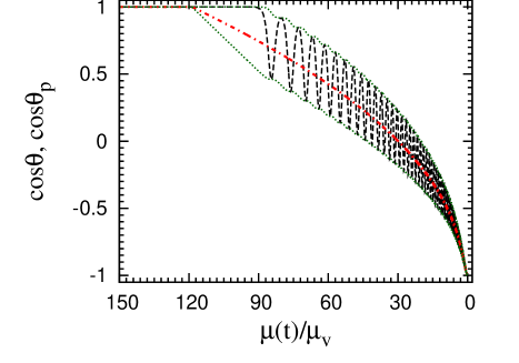
Figure 8: Nutation of the neutrino gyroscope shown in terms of $\cos\theta$ as a function of $\mu(t)/\mu_{\rm v}$ (dashed curve) for $\tilde{\theta}_{\rm v}=10^{-5}$ (IH). The gyroscope is characterized by $2\mu_{\rm v}/\delta m^{2}=1/9$ MeV^-1, $\alpha=2/3$, and $\mu(t)=\mu(0)\left\{1-\sqrt{1-[\tau/(t+\tau)]^{2}}\right\}^{2}$, where $\mu(0)/\mu_{\rm v}=2.52\times 10^{5}$ and $\tau=8.45/\mu_{\rm v}$. The dot-dashed curve is for $\cos\theta_{p}$, which corresponds to the minimum of the instantaneous $V_{\rm eff}(\theta)$, and the dotted curves are for $\cos\theta_{\rm max}$ and $\cos\theta_{\rm min}$, which correspond to $V_{\rm eff}(\theta)=E_{\theta}$.

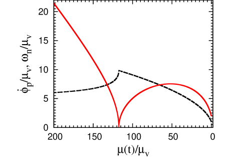
Figure 9: Dimensionless precession frequency $\dot{\phi}_{p}/\mu_{\rm v}$ (dashed curve) and nutation frequency $\omega_{n}/\mu_{\rm v}$ (solid curve) as functions of $\mu(t)/\mu_{\rm v}$ for the neutrino gyroscope shown in Fig. 8.

It can be seen from Fig. 8 that the general trend of $\theta$ follows the evolution of $\theta_{p}$. In other words, nutation of the neutrino gyroscope occurs around the minimum of the instantaneous $V_{\rm eff}(\theta)$ as $\mu(t)$ slowly decreases from a large initial value $\mu(0)\gg\mu_{\rm v}$. It is also clear that the motion of the gyroscope falls into two distinct regimes separated by a critical $\mu_{\rm cr}\approx 119\mu_{\rm v}$. For $\mu>\mu_{\rm cr}$, the nutation amplitude is extremely small and $\theta\approx\theta_{p}$ to very good approximation. As $\mu$ drops below $\mu_{\rm cr}$, $\theta$ initially stays small even as $\theta_{p}$ increases. This can be understood from Fig. 9, which shows that the nutation frequency $\omega_{n}$ is small at $\mu\sim\mu_{\rm cr}$ and is practically zero at $\mu_{\rm cr}$. As $\mu$ decreases further, $\omega_{n}$ becomes sufficiently large and $\theta$ starts to oscillate around $\theta_{p}$. The amplitude of this oscillation is also that of nutation and can be taken as $\eta\approx(\theta_{\rm max}-\theta_{\rm min})/2$. The longer $\omega_{n}$ stays small at $\mu\sim\mu_{\rm cr}$, the larger $\eta$ is for $\mu<\mu_{\rm cr}$.

We have constructed the series of gyroscopes for specific values of $\mu$ using the instantaneous $\mathbf{s}_{1}$ and $\mathbf{s}_{2}$ numerically calculated for the $\mu(t)$ in Eq. (36). In fact, so long as $\mu(t)$ slowly decreases from some large initial value $\mu(0)\gg\mu_{\rm v}$, the characteristics of such gyroscopes essentially depend on the values of $\mu$ but not the specific functional form of $\mu(t)$. To see this, we consider the set of parameters $\sigma$, $Q$, and $\theta_{p}$ that characterize the gyroscope at a specific value of $\mu$. We can choose three equations to solve for these parameters as follows. From the definitions of $\sigma$, $\mathbf{S}$, and $\mathbf{Q}$, we obtain

$$\sigma Q =\frac{1-\alpha^{2}}{4}-\frac{\mu_{\rm v}}{\mu}S_{z},$$ (37a)

$$S^{2}+Q^{2}+2\frac{\mu_{\rm v}}{\mu}Q\cos\theta+\left(\frac{\mu_{\rm v}}{\mu}\right)^{2} =\frac{1+\alpha^{2}}{2}.$$ (37b)

Applying Eqs. (25c) and (37b) to $\theta=\theta_{p}$, at which $\dot{\theta}$ reaches its maximum value of $(\dot{\theta})_{\rm max}\approx\eta\omega_{n}$ [see Eqs. (33a) and (33b)], we further obtain

$$\frac{\dot{\phi}_{p}}{\mu}\sin^{2}\theta_{p}+\sigma\cos\theta_{p} =S_{z},$$ (38a)

$$\left(\frac{\eta\omega_{n}}{\mu}\right)^{2}+\left(\frac{\dot{\phi}_{p}}{\mu}\right)^{2}\sin^{2}\theta_{p}+\sigma^{2}+Q^{2}+2\frac{\mu_{\rm v}}{\mu}Q\cos\theta_{p}+\left(\frac{\mu_{\rm v}}{\mu}\right)^{2} \approx\frac{1+\alpha^{2}}{2}.$$ (38b)

Treating $\eta$ as a small parameter and ignoring the $\eta^{2}$ term in Eq. (38b), we can solve this equation along with Eqs. (37a) and (38a) to obtain $\sigma$, $Q$, and $\theta_{p}$ [note that $\dot{\phi}_{p}$ is given in terms of $\sigma$, $Q$, and $\theta_{p}$ by Eq. (31); see Appendix A for a different but equivalent method to obtain these parameters]. As this approximate solution assumes $\eta=0$, it is a “pure-precession” solution Duan et al. (2007), for which the gyroscope always stays at the minimum of the instantaneous $V_{\rm eff}(\theta)$.

For $\tilde{\theta}_{\rm v}\ll 1$, the pure-precession solution gives

$$\theta_{p} \ll 1,$$ (39a)

$$\dot{\phi}_{p} \to\frac{1+\alpha}{1-\alpha}\mu_{\rm v},$$ (39b)

$$\omega_{n} \to\frac{1-\alpha}{2}\mu-2\left(\frac{1+\alpha}{1-\alpha}\right)\mu_{\rm v},$$ (39c)

at $\mu\gg\mu_{\rm v}$ (see Appendix B for more detailed discussion of the initial motion of the neutrino gyroscope), and

$$\theta_{p} \to\pi,$$ (40a)

$$\dot{\phi}_{p} \to\mu_{\rm v},$$ (40b)

$$\omega_{n} \to 2\mu_{\rm v},$$ (40c)

at $\mu\ll\mu_{\rm v}$. In general, the $\theta_{p}$, $\dot{\phi}_{p}$, and $\omega_{n}$ calculated for the pure-precession solution are within $\sim 1\%$ of the values shown in Figs. 8 and 9.

Equation (39c) suggests that $\omega_{n}$ becomes very small as $\mu$ decreases to some critical value $\mu_{\rm cr}$. In Appendix C, we show that

$$\mu_{\rm cr}=\frac{4\mu_{\rm v}}{\left(1-\sqrt{\alpha}\right)^{2}},$$ (41)

which is $\mu_{\rm cr}\approx 119\mu_{\rm v}$ for $\alpha=2/3$, in excellent agreement with Figs. 8 and 9. At $\mu=\mu_{\rm cr}$, we have (see Appendix C)

$$\theta_{p,{\rm cr}} \approx\frac{2\sqrt{2}\alpha^{1/6}}{(1+\sqrt{\alpha})^{2/3}}\tilde{\theta}_{\rm v}^{2/3},$$ (42a)

$$\dot{\phi}_{p,{\rm cr}} \approx\frac{\mu_{\rm cr}S_{z}}{2}\approx\frac{1+\sqrt{\alpha}}{1-\sqrt{\alpha}}\mu_{\rm v},$$ (42b)

$$\omega_{n,{\rm cr}} \approx\frac{\sqrt{3}}{2}\mu_{\rm cr}S_{z}\theta_{p,{\rm cr}}\approx\frac{2\sqrt{6}\alpha^{1/6}(1+\sqrt{\alpha})^{1/3}}{1-\sqrt{\alpha}}\tilde{\theta}_{\rm v}^{2/3}\mu_{\rm v}.$$ (42c)

As $\theta_{p}\ll 1$ at $\mu\gg\mu_{\rm v}$ and at $\mu=\mu_{\rm cr}$ for $\tilde{\theta}_{\rm v}\ll 1$, the neutrino gyroscope stays in the upright position and behaves like a sleeping top (e.g., Hannestad et al. (2006); Duan et al. (2007)) at $\mu\geq\mu_{\rm cr}$ (see Fig. 8).

IV Resonances Driven by The Neutrino Gyroscope

In this section we return to the system initially consisting of $\nu_{e}$ and $\bar{\nu}_{e}$ with spectra of the form in Eq. (1). As discussed in Secs. II.1 and II.2, the approximate mean field of NFIS’s for this system can be described by the neutrino gyroscope. We now try to understand the evolution of an individual NFIS in the system in terms of its response to the neutrino gyroscope. Specifically, we study the evolution of $\mathbf{s}_{\omega}$ governed by

$$\frac{d}{dt}\mathbf{s}_{\omega}=\mathbf{s}_{\omega}\times[\omega\mathbf{H}_{\rm v}-\mu(t)\mathbf{S}]=[\omega\mathbf{\hat{e}}_{z}^{\rm I}+\mu(t)\mathbf{S}]\times\mathbf{s}_{\omega},$$ (43)

where $\mathbf{S}$ is the total angular momentum of the neutrino gyroscope discussed in Sec. III.2.

IV.1 Precession-Driven Resonance

We first ignore nutation and consider only precession of the neutrino gyroscope. With $\eta=0$ (and $\gamma=0$ as noted in Sec. III.1), Eq. (35) becomes

$$S_{x}+iS_{y}\approx iS_{\perp}\exp(i\dot{\phi}_{p}t),$$ (44)

where

$$S_{\perp}=\left(\frac{\dot{\phi}_{p}}{\mu}\cos\theta_{p}-\sigma\right)\sin\theta_{p}.$$ (45)

Equation (44) represents a vector rotating in the $xy$-plane of Frame I. Let Frame II rotate with an angular velocity $\dot{\phi}_{p}\mathbf{\hat{e}}_{z}^{\rm I}$ relative to Frame I. Then $\mathbf{S}$ is a non-rotating vector in Frame II and can be chosen as

$$\mathbf{S}\approx S_{z}\mathbf{\hat{e}}_{z}^{\rm I}+S_{\perp}\mathbf{\hat{e}}_{y}^{\rm II},$$ (46)

where $\mathbf{\hat{e}}_{y}^{\rm II}$ is the unit vector in the $y$-direction of Frame II (see Fig. 10). We rewrite Eq. (43) in this frame as

$$\frac{d}{dt}\mathbf{s}_{\omega}=[(\omega+\mu S_{z}-\dot{\phi}_{p})\mathbf{\hat{e}}_{z}^{\rm I}+\mu S_{\perp}\mathbf{\hat{e}}_{y}^{\rm II}]\times\mathbf{s}_{\omega}\equiv\mathbf{H}_{\rm II}\times\mathbf{s}_{\omega}.$$ (47)

Note that in the above equation $\omega$ and $S_{z}$ are constants but $\dot{\phi}_{p}$ and $S_{\perp}$ are functions of $\mu(t)$. A resonance occurs when the $z$-component of $\mathbf{H}_{\rm II}$ vanishes. We refer to this as the precession-driven resonance. We denote the value of $\mu$ at which an individual NFIS $\mathbf{s}_{\omega}$ goes through this resonance as $\mu_{{\rm res},p}$, which can be obtained from

$$\omega=\dot{\phi}_{p}(\mu_{{\rm res},p})-\mu_{{\rm res},p}S_{z}.$$ (48)

Here $\dot{\phi}_{p}(\mu_{{\rm res},p})$ is the value of $\dot{\phi}_{p}$ at $\mu=\mu_{{\rm res},p}$. Using the neutrino gyroscope in Fig. 8, we show $\mu_{{\rm res},p}/\mu_{\rm v}$ as a function of $\omega/\mu_{\rm v}$ (solid curve) in Fig. 11 (note that the pure-precession solution gives essentially the same result).

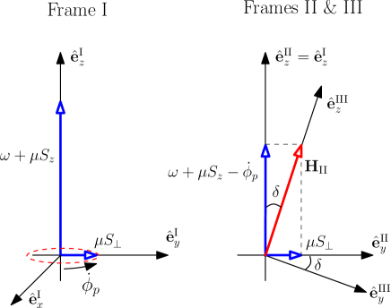
Figure 10: Illustration of relations among Frames I, II, and III. Frame I is fixed to the laboratory. Frame II has the same $z$-axis as Frame I and rotates around this axis with an angular velocity $\dot{\phi}_{p}\mathbf{\hat{e}}_{z}^{\rm I}$ relative to Frame I. When only precession of the neutrino gyroscope is considered, the net effective field interacting with an individual NFIS $\mathbf{s}_{\omega}$ has two components in Frame I: one fixed in the direction of $\mathbf{\hat{e}}_{z}^{\rm I}$ and the other rotating with an angular velocity $\dot{\phi}_{p}\mathbf{\hat{e}}_{z}^{\rm I}$. It is convenient to use Frame II to discuss the precession-driven resonance as the net effective field becomes a non-rotating vector $\mathbf{H}_{\rm II}$ in this frame. Frame III has the same $x$-axis as Frame II but its $z$-axis is in the direction of $\mathbf{H}_{\rm II}$, which makes an angle $\delta$ with respect to $\mathbf{\hat{e}}_{z}^{\rm I}$. Frame III is used in discussing the nutation-driven resonance. See text for details.

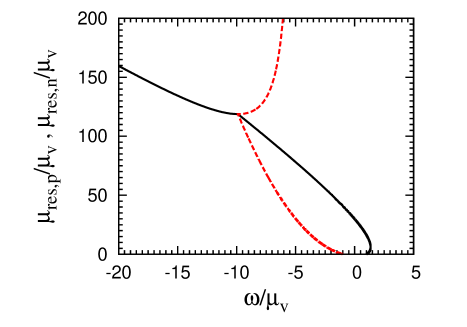
Figure 11: Values of $\mu_{{\rm res},p}/\mu_{\rm v}$ (solid curve) and $\mu_{{\rm res},n}/\mu_{\rm v}$ (dashed curve) as functions of $\omega/\mu_{\rm v}$. An NFIS $\mathbf{s}_{\omega}$ goes through the precession-driven (nutation-driven) resonance at $\mu=\mu_{{\rm res},p}$ ($\mu_{{\rm res},n}$) as the neutrino gyroscope in Fig. 8 evolves through $\mu(t)$.

The evolution of $\mathbf{s}_{\omega}$ in Frame II based on Eq. (47) is very similar to the MSW effect (see Fig. 12). At a specific time $t$, $\mathbf{s}_{\omega}$ precesses around the instantaneous $\mathbf{H}_{\rm II}$ with an angular velocity $\mathbf{H}_{\rm II}$. For slowly varying $\mu(t)$, the evolution of $\mathbf{s}_{\omega}$ is adiabatic in that the precession adjusts to the instantaneous angular velocity (the direction and magnitude of which are both changing slowly in general) but the angle between $\mathbf{s}_{\omega}$ and $\mathbf{H}_{\rm II}$ remains fixed. Therefore, the initial $\nu_{e}$ or $\bar{\nu}_{e}$ represented by $\mathbf{s}_{\omega}$ remains in the same flavor following adiabatic evolution if the initial and final directions of $\mathbf{H}_{\rm II}$ are the same, but is fully converted into a $\nu_{x}$ or $\bar{\nu}_{x}$ if the initial and final directions of $\mathbf{H}_{\rm II}$ are opposite. For the neutrino gyroscope under consideration, $\mathbf{H}_{\rm II}\approx\mu S_{z}\mathbf{\hat{e}}_{z}^{\rm I}$ at $t=0$ corresponding to $\mu\gg\mu_{\rm v}$, where we have used $\mu S_{z}\gg|\omega|,\dot{\phi}_{p},\mu|S_{\perp}|$ in this limit. At large times corresponding to $\mu\ll\mu_{\rm v}$, $\mathbf{H}_{\rm II}\approx(\omega-\mu_{\rm v})\mathbf{\hat{e}}_{z}^{\rm I}$, where we have used $\dot{\phi}_{p}=\mu_{\rm v}$ in this limit. Consequently, the initial and final directions of $\mathbf{H}_{\rm II}$ are the same for $\omega>\mu_{\rm v}$ but are opposite for $\omega<\mu_{\rm v}$. In the latter case, a precession-driven resonance occurs when the $z$-component of $\mathbf{H}_{\rm II}$ vanishes before the direction of $\mathbf{H}_{\rm II}$ is reversed (see Fig. 12). Thus, when only precession-driven resonance matters and adiabatic evolution applies, an initial $\nu_{e}$ with $\omega>\mu_{\rm v}$ remains as a $\nu_{e}$, while an initial $\nu_{e}$ with $\omega<\mu_{\rm v}$ or an initial $\bar{\nu}_{e}$ (with $\omega<0$) is fully converted into a $\nu_{x}$ or $\bar{\nu}_{x}$, respectively. This is basically the explanation for the stepwise spectral swap originally discovered in Duan et al. (2006b) (see also discussion in Raffelt and Smirnov (2007a)).

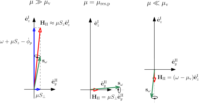
Figure 12: Illustration of nearly full conversion of an initial $\nu_{e}$ represented by $\mathbf{s}_{\omega}$ with $\omega<\mu_{\rm v}$ following adiabatic evolution through a precession-driven resonance. In Frame II, adiabatic evolution corresponds to precession of $\mathbf{s}_{\omega}$ around $\mathbf{H}_{\rm II}$ with a fixed angle between the two vectors. At $\mu\gg\mu_{\rm v}$, $\mathbf{H}_{\rm II}$ nearly coincides with $\mathbf{\hat{e}}_{z}^{\rm I}$. At $\mu=\mu_{{\rm res},p}$ corresponding to the resonance, the $z$-component of $\mathbf{H}_{\rm II}$ vanishes. At $\mu\ll\mu_{\rm v}$, $\mathbf{H}_{\rm II}$ is opposite to $\mathbf{\hat{e}}_{z}^{\rm I}$ for $\omega<\mu_{\rm v}$. Consequently, the initial and final directions of $\mathbf{H}_{\rm II}$ are nearly opposite, and the same is true of $\mathbf{s}_{\omega}$.

For adiabatic evolution, the rate at which the direction of $\mathbf{H}_{\rm II}$ changes must be slow compared with the precession frequency of $\mathbf{s}_{\omega}$:

$$\left|\frac{d}{dt}\frac{\mathbf{H}_{\rm II}}{|\mathbf{H}_{\rm II}|}\right|=\frac{|\mathbf{H}_{\rm II}\times d\mathbf{H}_{\rm II}/dt|}{|\mathbf{H}_{\rm II}|^{2}}\ll|\mathbf{H}_{\rm II}|.$$ (49)

The above condition is most stringent at resonance when the $z$-component of $\mathbf{H}_{\rm II}$ vanishes and $|\mathbf{H}_{\rm II}|$ becomes very small (see Fig. 12). We define the adiabaticity parameter for this precession-driven resonance as

$$\lambda_{p}\equiv\frac{|\mathbf{H}_{\rm II}\times d\mathbf{H}_{\rm II}/dt|_{\rm res}}{|\mathbf{H}_{\rm II}|_{\rm res}^{3}}=\frac{|d(\dot{\phi}_{p}-\mu S_{z})/dt|}{(\mu S_{\perp})^{2}}.$$ (50)

Adiabatic evolution obtains for $\lambda_{p}\ll 1$ (note that $\lambda_{p}$ is defined differently from the usual adiabaticity parameter for the conventional MSW effect). Using the neutrino gyroscope in Fig. 8, we show $\lambda_{p}$ as a function of $\mu(t)/\mu_{\rm v}$ (solid curve) in Fig. 13. It can be seen from this figure that evolution through the precession-driven resonance is adiabatic at $\mu<115\mu_{\rm v}$, but is extremely non-adiabatic at $\mu\gtrsim\mu_{\rm cr}\approx 119\mu_{\rm v}$. As $\mu\gtrsim\mu_{\rm cr}$ corresponds to the sleeping-top regime with $\theta_{p}\ll 1$, the small values of $S_{\perp}\propto\sin\theta_{p}$ [see Eq. (45)] result in $\lambda_{p}\gg 1$ in this regime.

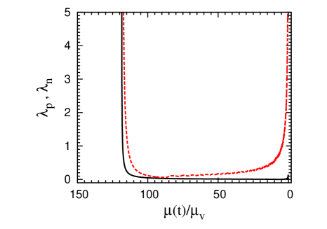
Figure 13: Adiabaticity parameters $\lambda_{p}$ (solid curve) and $\lambda_{n}$ (dashed curve) for evolution through precession-driven and nutation-driven resonances, respectively, as functions of $\mu(t)/\mu_{\rm v}$ for the neutrino gyroscope shown in Fig. 8.

IV.2 Nutation-Driven Resonance

Now we consider both precession and nutation of the neutrino gyroscope. The terms proportional to $\eta$ in Eq. (35) contain the factors $\exp(i\omega_{n}t)$ and $\exp(-i\omega_{n}t)$, which correspond to rotation with angular velocities $\omega_{n}\mathbf{\hat{e}}_{z}^{\rm I}$ and $-\omega_{n}\mathbf{\hat{e}}_{z}^{\rm I}$, respectively, relative to Frame II. However, frames rotating with these angular velocities are not convenient to use because $\mu(t)S_{\perp}\mathbf{\hat{e}}_{y}^{\rm II}$, and hence $\mathbf{H}_{\rm II}$, rotate in such frames. To find the appropriate frames, we first consider Frame III with its axes defined by the unit vectors (see Fig. 10)

$$\mathbf{\hat{e}}_{x}^{\rm III} =\mathbf{\hat{e}}_{x}^{\rm II},$$ (51a)

$$\mathbf{\hat{e}}_{y}^{\rm III} =\cos\delta\mathbf{\hat{e}}_{y}^{\rm II}-\sin\delta\mathbf{\hat{e}}_{z}^{\rm I},$$ (51b)

$$\mathbf{\hat{e}}_{z}^{\rm III} =\mathbf{H}_{\rm II}/|\mathbf{H}_{\rm II}|=\sin\delta\mathbf{\hat{e}}_{y}^{\rm II}+\cos\delta\mathbf{\hat{e}}_{z}^{\rm I},$$ (51c)

where

$$\cos\delta =\frac{\omega+\mu S_{z}-\dot{\phi}_{p}}{|\mathbf{H}_{\rm II}|},$$ (52a)

$$\sin\delta =\frac{\mu S_{\perp}}{|\mathbf{H}_{\rm II}|}.$$ (52b)

Note that just like Frame II, Frame III also rotates with an angular velocity $\dot{\phi}_{p}\mathbf{\hat{e}}_{z}^{\rm I}$ relative to Frame I. Using Eq. (35) (with $\beta=\gamma=0$ as noted in Sec. III.1), we write $\mathbf{S}$ in Frame III as

$$\mathbf{S} \approx S_{z}\mathbf{\hat{e}}_{z}^{\rm I}+S_{\perp}\mathbf{\hat{e}}_{y}^{\rm II}+\eta\frac{\dot{\phi}_{p}}{\mu}\sin\delta\cos(\omega_{n}t)\mathbf{\hat{e}}_{z}^{\rm III}$$

$$+\eta\frac{\dot{\phi}_{p}}{\mu}\frac{2\dot{\phi}_{p}-\mu S_{z}}{\omega_{n}}\sin(\omega_{n}t)\mathbf{\hat{e}}_{x}^{\rm III}+\eta\frac{\dot{\phi}_{p}}{\mu}\cos\delta\cos(\omega_{n}t)\mathbf{\hat{e}}_{y}^{\rm III}.$$ (53)

The last two terms in the above expression can be rewritten as two vectors rotating with angular velocities $\omega_{n}\mathbf{\hat{e}}_{z}^{\rm III}$ and $-\omega_{n}\mathbf{\hat{e}}_{z}^{\rm III}$, respectively, relative to Frame III:

$$(S_{x}+iS^{\prime}_{y})_{\rm III}\equiv i\frac{\eta}{2}\frac{\dot{\phi}_{p}}{\mu}\left[\left(\cos\delta-\frac{2\dot{\phi}_{p}-\mu S_{z}}{\omega_{n}}\right)e^{i\omega_{n}t}+\left(\cos\delta+\frac{2\dot{\phi}_{p}-\mu S_{z}}{\omega_{n}}\right)e^{-i\omega_{n}t}\right].$$ (54)

As we will see shortly, a new resonance occurs for $|\mathbf{H}_{\rm II}|=\omega_{n}$. Using Eqs. (30b), (31), (38a), and (47), we can rewrite the above resonance condition as:

$$(\omega+\dot{\phi}_{p})(\omega+2\mu S_{z}-3\dot{\phi}_{p})=0.$$ (55)

The term with the factor $\exp(-i\omega_{n}t)$ in Eq. (54) vanishes for $\omega=-\dot{\phi}_{p}$, while that with the factor $\exp(i\omega_{n}t)$ vanishes for $\omega=3\dot{\phi}_{p}-2\mu S_{z}$. We will see that the new resonance corresponds to $\omega=-\dot{\phi}_{p}$. So we can ignore the term with the factor $\exp(-i\omega_{n}t)$ in Eq. (54) when treating this resonance. We choose Frame IV to rotate with an angular velocity $\omega_{n}\mathbf{\hat{e}}_{z}^{\rm III}$ relative to Frame III. The term with the factor $\exp(i\omega_{n}t)$ in Eq. (54) represents a vector parallel to the unit vector $\mathbf{\hat{e}}_{y}^{\rm IV}$ in the $y$-direction of Frame IV. In this frame Eq. (43) effectively becomes

$$\frac{d}{dt}\mathbf{s}_{\omega}=\left[\left(|\mathbf{H}_{\rm II}|-\omega_{n}+\eta\dot{\phi}_{p}\sin\delta\cos\omega_{n}t\right)\mathbf{\hat{e}}_{z}^{\rm III}+\frac{\eta\dot{\phi}_{p}}{2}\left(\cos\delta-\frac{2\dot{\phi}_{p}-\mu S_{z}}{\omega_{n}}\right)\mathbf{\hat{e}}_{y}^{\rm IV}\right]\times\mathbf{s}_{\omega}.$$ (56)

It can be seen that a new resonance indeed occurs when $|\mathbf{H}_{\rm II}|=\omega_{n}$ if we ignore the small contribution proportional to $\eta$ in the term associated with $\mathbf{\hat{e}}_{z}^{\rm III}$ in the above equation. We refer to this as the nutation-driven resonance because it is driven by the nutation-dependent component of $\mathbf{S}$. We denote the value of $\mu$ at which an individual NFIS $\mathbf{s}_{\omega}$ goes through this resonance as $\mu_{{\rm res},n}$, which can be obtained from

$$\omega=-\dot{\phi}_{p}(\mu_{{\rm res},n}).$$ (57)

Here $\dot{\phi}_{p}(\mu_{{\rm res},n})$ is the value of $\dot{\phi}_{p}$ at $\mu=\mu_{{\rm res},n}$. Using the neutrino gyroscope in Fig. 8, we show $\mu_{{\rm res},n}/\mu_{\rm v}$ as a function of $\omega/\mu_{\rm v}$ (dashed curve) in Fig. 11 (note again that the pure-precession solution gives essentially the same result).

To see that $\omega=3\dot{\phi}_{p}-2\mu S_{z}$, which also gives $|\mathbf{H}_{\rm II}|=\omega_{n}$, does not correspond to a resonance, we recall that the term with the factor $\exp(i\omega_{n}t)$ in Eq. (54) vanishes for this $\omega$. We choose Frame V to rotate with an angular velocity $-\omega_{n}\mathbf{\hat{e}}_{z}^{\rm III}$ relative to Frame III and rewrite Eq. (43) in Frame V effectively as

$$\frac{d}{dt}\mathbf{s}_{\omega}=\left[\left(|\mathbf{H}_{\rm II}|+\omega_{n}+\eta\dot{\phi}_{p}\sin\delta\cos\omega_{n}t\right)\mathbf{\hat{e}}_{z}^{\rm III}+\frac{\eta\dot{\phi}_{p}}{2}\left(\cos\delta+\frac{2\dot{\phi}_{p}-\mu S_{z}}{\omega_{n}}\right)\mathbf{\hat{e}}_{y}^{\rm V}\right]\times\mathbf{s}_{\omega},$$ (58)

where $\mathbf{\hat{e}}_{y}^{\rm V}$ is the unit vector in the $y$-direction of Frame V. It can be seen that the term associated with $\mathbf{\hat{e}}_{z}^{\rm III}$ in the above equation never vanishes, and consequently, there is no resonance for $\omega=3\dot{\phi}_{p}-2\mu S_{z}$.

The adiabaticity for evolution through the nutation-driven resonance can be discussed similarly to the case of precession-driven resonance studied in Sec. IV.1. The evolution of $\mathbf{s}_{\omega}$ in Frame IV is governed by

$$\frac{d}{dt}\mathbf{s}_{\omega}=\mathbf{H}_{\rm IV}\times\mathbf{s}_{\omega}.$$ (59)

At resonance $\mathbf{H}_{\rm IV}$ is given by

$$(\mathbf{H}_{\rm IV})_{\rm res}\approx\eta\dot{\phi}_{p}\left(\frac{\mu S_{z}-2\dot{\phi}_{p}}{\omega_{n}}\right)\mathbf{\hat{e}}_{y}^{\rm IV}.$$ (60)

We define the adiabaticity parameter for the nutation-driven resonance as

$$\lambda_{n}\equiv\frac{|\mathbf{H}_{\rm IV}\times d\mathbf{H}_{\rm IV}/dt|_{\rm res}}{|\mathbf{H}_{\rm IV}|_{\rm res}^{3}}\approx\frac{|d(|\mathbf{H}_{\rm II}|-\omega_{n})/dt|_{\rm res}}{|\mathbf{H}_{\rm IV}|_{\rm res}^{2}}.$$ (61)

In Eqs.(60) and (61), we have neglected oscillatory terms proportional to $\eta$. Using the neutrino gyroscope in Fig. 8, we show $\lambda_{n}$ as a function of $\mu/\mu_{\rm v}$ (dashed curve) in Fig. 13. It can be seen from this figure that evolution through the nutation-driven resonance is adiabatic at $\mu/\mu_{\rm v}\sim 10$–110 and becomes non-adiabatic outside this range. In particular, evolution is extremely non-adiabatic at $\mu\gtrsim\mu_{\rm cr}\approx 119\mu_{\rm v}$ and at $\mu\lesssim 5\mu_{\rm v}$ as the very small nutation amplitude $\eta$ (see Fig. 8) results in $\lambda_{n}\gg 1$ in these two regimes.

IV.3 Evolution through Resonances Driven by the Neutrino Gyroscope

Based on the discussion in Secs. IV.1 and IV.2, an NFIS may experience two types of resonances driven by precession and nutation of the neutrino gyroscope, respectively. For the NFIS $\mathbf{s}_{\omega}$, a precession-driven resonance occurs at $\omega=\dot{\phi}_{p}(\mu_{{\rm res},p})-\mu_{{\rm res},p}S_{z}$, and a nutation-driven resonance occurs at $\omega=-\dot{\phi}_{p}(\mu_{{\rm res},n})$. Formally these two resonances coincide at $\mu_{{\rm res},p}=\mu_{{\rm res},n}=\mu_{\rm cr}$ for $\omega=\omega_{\rm cr}\equiv-\dot{\phi}_{p,{\rm cr}}\approx(1+\sqrt{\alpha})\mu_{\rm v}/(1-\sqrt{\alpha})$ [see Eq. (42b)]. Noting that $\dot{\phi}_{p}\to(1+\alpha)\mu_{\rm v}/(1-\alpha)$ at $\mu\gg\mu_{\rm cr}$ [see Eq. (39b)] and $\dot{\phi}_{p}\to\mu_{\rm v}$ at $\mu\ll\mu_{\rm v}$ [see Eq. (40b)], we introduce $\omega_{A}\equiv-(1+\alpha)\mu_{\rm v}/(1-\alpha)$, $\omega_{B}\equiv-\mu_{\rm v}$, and $\omega_{C}\equiv\mu_{\rm v}$ to define ranges of $\omega$ with different resonances. It turns out that for $\omega=\omega_{D}$ slightly larger than $\omega_{C}$, there are two possible values for $\mu_{{\rm res},p}$. Altogether, the varieties of resonances experienced by $\mathbf{s}_{\omega}$ can be classified into six categories:

• for $\omega<\omega_{\rm cr}$, $\mathbf{s}_{\omega}$ experiences only a precession-driven resonance at $\mu_{{\rm res},p}>\mu_{\rm cr}$;

• for $\omega_{\rm cr}<\omega<\omega_{A}$, $\mathbf{s}_{\omega}$ experiences a nutation-driven resonance at $\mu_{{\rm res},n}>\mu_{\rm cr}$, then a precession-driven resonance at $\mu_{{\rm res},p}<\mu_{\rm cr}$, and finally a second nutation-driven resonance at $\mu_{{\rm res},n}^{\prime}<\mu_{{\rm res},p}$;

• for $\omega_{A}<\omega<\omega_{B}$, $\mathbf{s}_{\omega}$ experiences a precession-driven resonance at $\mu_{{\rm res},p}<\mu_{\rm cr}$ followed by a nutation-driven resonance at $\mu_{{\rm res},n}<\mu_{{\rm res},p}$;

• for $\omega_{B}<\omega<\omega_{C}$, $\mathbf{s}_{\omega}$ experiences only a precession-driven resonance at $\mu_{{\rm res},p}<\mu_{\rm cr}$;

• for $\omega_{C}<\omega<\omega_{D}$, $\mathbf{s}_{\omega}$ experiences two precession-driven resonances at $\mu_{{\rm res},p}<\mu_{\rm cr}$ and $\mu_{{\rm res},p}^{\prime}<\mu_{{\rm res},p}$, respectively.

• for $\omega>\omega_{D}$, $\mathbf{s}_{\omega}$ does not experience any resonance.

For the neutrino gyroscope in Fig. 8, $\mu_{\rm cr}\approx 119\mu_{\rm v}$, $\omega_{\rm cr}\approx-10\mu_{\rm v}$, $\omega_{A}\approx-5\mu_{\rm v}$, and $\omega_{D}\approx 1.5\mu_{\rm v}$. The six categories of resonances for this example are shown in the top left panel of Fig. 14.

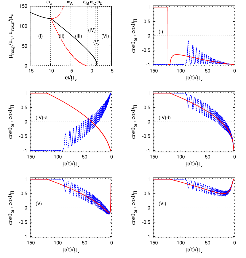
Figure 14: Ranges I–VI of $\omega$ based on occurrences of precession-driven (solid curve) and nutation-driven (dashed curve) resonances (top left panel) and example evolution of $\cos\theta_{\omega}$ (dashed curves) and $\cos\theta_{\rm II}$ (solid curves) as functions of $\mu(t)/\mu_{\rm v}$ for $\omega/\mu_{\rm v}=-12$ (I), $-0.5$ (IV-a), 0.5 (IV-b), 1.1 (V), and 3 (VI), respectively. See text for details.

Only precession-driven resonances are involved for $\omega$ in ranges I, IV, and V, and there are no resonances for $\omega$ in range VI. We first consider the overall evolution of $\mathbf{s}_{\omega}$ for $\omega$ in these ranges using the neutrino gyroscope in Fig. 8. As nutation is unimportant for these cases, we focus on $\mathbf{H}_{\rm II}$ as the net effective field interacting with $\mathbf{s}_{\omega}$ [see Eq. (47)]. At $\mu=\mu(0)\gg\mu_{\rm cr}$, $\mathbf{H}_{\rm II}$ is essentially in the direction of $\mathbf{\hat{e}}_{z}^{\rm I}$ and $\mathbf{s}_{\omega}$ is either aligned (initial $\nu_{e}$, $\omega>0$) or anti-aligned (initial $\bar{\nu}_{e}$, $\omega<0$) with $\mathbf{H}_{\rm II}$. We show the subsequent evolution of $\mathbf{s}_{\omega}$ relative to $\mathbf{H}_{\rm II}$ by comparing $\cos\theta_{\omega}\equiv\mathbf{s}_{\omega}\cdot\mathbf{\hat{e}}_{z}^{\rm I}/|\mathbf{s}_{\omega}|$ (dashed curve) with $\cos\theta_{\rm II}\equiv\mathbf{H}_{\rm II}\cdot\mathbf{\hat{e}}_{z}^{\rm I}/|\mathbf{H}_{\rm II}|$ (solid curve) in Fig. 14. For $\omega/\mu_{\rm v}=-12$ in range I, $\mathbf{s}_{\omega}$ is initially anti-aligned with $\mathbf{H}_{\rm II}$ ($\cos\theta_{\omega}\approx-1$ but $\cos\theta_{\rm II}\approx 1$). At $\mu/\mu_{\rm v}\approx 122$, $\cos\theta_{\rm II}$ vanishes and a resonance occurs. However, evolution through this resonance is extremely non-adiabatic (see Fig. 13). Consequently, $\cos\theta_{\omega}$ is unaffected while $\cos\theta_{\rm II}$ changes drastically from $\approx 1$ to $\approx-1$ immediately after the resonance. Subsequent evolution of $\mathbf{s}_{\omega}$ is essentially adiabatic with $\cos\theta_{\omega}$ oscillating around $\cos\theta_{\rm II}$ and eventually settling to $\approx-1$ again. This kind of evolution applies to all $\omega$ in range I, for which there is no net flavor transformation. For $\omega/\mu_{\rm v}=-0.5$ (0.5) in range IV, there is a resonance at $\mu/\mu_{\rm v}\approx 36$ (24). Evolution through the resonance is adiabatic (see Fig. 13) and $\mathbf{s}_{\omega}$ stays anti-aligned (aligned) with $\mathbf{H}_{\rm II}$ during the entire evolution. As the initial and final directions of $\mathbf{H}_{\rm II}$ are opposite, there is full flavor conversion for $\omega$ in range IV. For $\omega/\mu_{\rm v}=1.1$ in range V, there are two resonances at $\mu/\mu_{\rm v}\approx 14$ and 1, respectively. Evolution through both resonances is essentially adiabatic (see Fig. 13) and $\mathbf{s}_{\omega}$ stays aligned with $\mathbf{H}_{\rm II}$ during the entire evolution. As $\cos\theta_{\rm II}$ changes sign twice, the initial and final directions of $\mathbf{H}_{\rm II}$ are the same and there is no net flavor transformation for $\omega$ in range V. Finally, for $\omega/\mu_{\rm v}=3$ in range VI, there is no resonance and evolution is adiabatic. So $\cos\theta_{\omega}$ oscillates around $\cos\theta_{\rm II}$, indicating that $\mathbf{s}_{\omega}$ is always aligned with $\mathbf{H}_{\rm II}$. There is no net flavor transformation for $\omega$ in range VI.

Resonances driven by both precession and nutation of the neutrino gyroscope are involved for $\omega$ in ranges II and III. We discuss the evolution of $\mathbf{s}_{\omega}$ for these ranges using $\mathbf{H}_{\rm IV}$ as the net effective field. We define $\cos\theta_{\rm IV}\equiv\mathbf{H}_{\rm IV}\cdot\mathbf{\hat{e}}_{z}^{\rm I}/|\mathbf{H}_{\rm IV}|$. Neglecting terms proportional to $\eta$, we obtain $\cos\theta_{\rm IV}\approx{\rm sgn}(|\mathbf{H}_{\rm II}|-\omega_{n})\cos\theta_{\rm II}$ (see Sec. IV.2), where sgn$(x)$ is the sign of $x$. Using the neutrino gyroscope in Fig. 8, we compare the evolution of $\cos\theta_{\omega}$ and $\cos\theta_{\rm IV}$ for $\omega$ in ranges II and III in Fig. 15. For $\omega/\mu_{\rm v}=-6$ in range II, $\mathbf{s}_{\omega}$ is initially aligned with $\mathbf{H}_{\rm IV}$. A nutation-driven resonance occurs at $\mu/\mu_{\rm v}\approx 210$. However, evolution through this resonance is extremely non-adiabatic (see Fig. 13). So $\cos\theta_{\omega}$ is unaffected although $\cos\theta_{\rm IV}$ jumps from $\approx-1$ to $\approx 1$ immediately after the resonance. Then $\cos\theta_{\rm IV}$ vanishes at $\mu/\mu_{\rm v}\approx 99$ corresponding to $\omega=3\dot{\phi}_{p}-2\mu S_{z}$ and $|\mathbf{H}_{\rm II}|=\omega_{n}$, but this is not a resonance (see Sec. IV.2). A precession-driven resonance occurs at $\mu/\mu_{\rm v}\approx 86$ and a second nutation-driven resonance occurs at $\mu/\mu_{\rm v}\approx 43$. Evolution through both these resonances is adiabatic (see Fig. 13). Consequently, at $\mu/\mu_{\rm v}<99$, $\cos\theta_{\omega}$ oscillate around $\cos\theta_{\rm IV}$, eventually settling to $\approx-1$ again. There is no net flavor transformation for $\omega$ in range II. For $\omega/\mu_{\rm v}=-4$ in range III, $\cos\theta_{\rm IV}$ vanishes at $\mu/\mu_{\rm v}\approx 89$, which is not a resonance. A precession-driven resonance occurs at at $\mu/\mu_{\rm v}\approx 69$ and a nutation-driven resonance occurs at $\mu/\mu_{\rm v}\approx 19$. Evolution is adiabatic throughout and there is no net flavor transformation. For $\omega/\mu_{\rm v}=-2$ also in range III, the evolution of $\cos\theta_{\rm IV}$ is similar to that for $\omega/\mu_{\rm v}=-4$. However, for $\omega/\mu_{\rm v}=-2$, evolution through the precession-driven resonance at $\mu/\mu_{\rm v}\approx 51$ is adiabatic while that through the nutation-driven resonance at $\mu/\mu_{\rm v}\approx 4$ is non-adiabatic (see Fig. 13). This kind of evolution applies to $-3<\omega/\mu_{\rm v}<-1$ and results in significant flavor transformation.

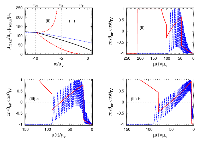
Figure 15: Ranges II and III of $\omega$ based on occurrences of precession-driven (solid curve) and nutation-driven (dashed curve) resonances (top left panel) and example evolution of $\cos\theta_{\omega}$ (dashed curves) and $\cos\theta_{\rm IV}$ (solid curves) as functions of $\mu(t)/\mu_{\rm v}$ for $\omega/\mu_{\rm v}=-6$ (II), $-4$ (III-a), and $-2$ (III-b), respectively. The dotted curve in the top left panel shows the value of $\mu/\mu_{\rm v}$ for which $\omega=3\dot{\phi}_{p}-2\mu S_{z}$ as a function of $\omega/\mu_{\rm v}$. Note that no resonance occurs at this $\mu$ although the corresponding $\cos\theta_{\rm IV}$ vanishes. See text for details.

In summary, evolution of $\mathbf{s}_{\omega}$ can be understood in terms of the resonances it experiences. A resonance does not affect the net flavor transformation if evolution through it is very non-adiabatic. Net full flavor conversion results from adiabatic evolution through an odd number of resonances while little net flavor transformation results from adiabatic evolution through an even number (including zero) of resonances. As discussed in Secs. IV.1 and IV.2, evolution through a resonance driven by either precession or nutation at $\mu>\mu_{\rm cr}$ is extremely non-adiabatic. In contrast, evolution through a precession-driven resonance at $\mu<\mu_{\rm cr}$ is essentially always adiabatic. We introduce a parameter $\mu_{\rm tr}$ to discuss the adiabaticity of evolution through a nutation-driven resonance at $\mu<\mu_{\rm cr}$: the evolution is adiabatic (non-adiabatic) when such a resonance occurs at $\mu_{\rm tr}<\mu<\mu_{\rm cr}$ ($\mu<\mu_{\rm tr}$). We choose $\mu_{\rm tr}$ to correspond to an adiabaticity parameter $\lambda_{n}=0.5$. For the neutrino gyroscope in Fig. 8, $\mu_{\rm tr}\approx 12\mu_{\rm v}$ and $\mathbf{s}_{\omega}$ with $\omega\approx-3\mu_{\rm v}$ goes through a nutation-driven resonance at $\mu=\mu_{\rm tr}$ (see Figs. 11 and 13).

Now the swap factor shown as the dashed curve in Fig. 6 can be understood based on the above discussion and the occurrences of resonances listed in the beginning of this subsection and shown in Figs. 14 and 15. This curve is re-plotted as the solid curve in Fig. 16b with ranges I to VI for $\omega$ indicated. Recall that $f_{S}^{(0)}\approx-1$ corresponds to nearly full flavor transformation. This applies to $\omega$ in range IV, for which there is only a single precession-driven resonance at $\mu<\mu_{\rm cr}$ and evolution through this resonance is adiabatic. A variety of evolution results in $f_{S}^{(0)}\approx 1$ corresponding to little net flavor transformation for $\omega$ in ranges I, II, V, and VI: non-adiabatic evolution through a single precession-driven resonance at $\mu>\mu_{\rm cr}$ (I), non-adiabatic evolution through a nutation-driven resonance at $\mu>\mu_{\rm cr}$ followed by adiabatic evolution through a precession-driven resonance and a second nutation-driven resonance at $\mu<\mu_{\rm cr}$ (II), adiabatic evolution through two precession-driven resonances at $\mu<\mu_{\rm cr}$ (V), and adiabatic evolution with no resonance (VI). A precession-driven resonance and a nutation-driven resonance occur at $\mu<\mu_{\rm cr}$ for $\omega$ in range III and evolution through the precession-driven resonance is always adiabatic. However, evolution through the nutation-driven resonance is adiabatic only for $\omega<-3\mu_{\rm v}$ in this range and becomes more and more non-adiabatic as $\omega$ increases above $\sim-3\mu_{\rm v}$. Consequently, a transition from $f_{S}^{(0)}\approx 1$ towards $-1$ occurs at $\omega\sim-3\mu_{\rm v}$ in range III.

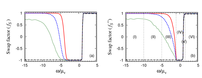
Figure 16: Comparison of the swap factors $f_{S}(\omega,t)$ (a) and $f_{S}^{(0)}(\omega,t)$ (b) at $r=250$ km for the system initially consisting of $\nu_{e}$ and $\bar{\nu}_{e}$ only as in Fig. 6. The solid, dashed, dotted, and dot-dashed curves are for $\tilde{\theta}_{\rm v}=10^{-5}$, $10^{-3}$, $10^{-2}$, and $10^{-1}$, respectively. Ranges I–VI of $\omega$ shown in (b) are based on occurrences of precession-driven and nutation-driven resonances (calculated for $\tilde{\theta}_{\rm v}=10^{-5}$ but valid for $\tilde{\theta}_{\rm v}\ll 1$).

IV.4 Application to System of Neutrinos with Continuous Spectra

As discussed in Sec. II.2, the total angular momentum of the neutrino gyroscope, which we denote as $\mathbf{S}^{(0)}$ again for clarity, approximates the mean field $\mathbf{S}$ of the NFIS’s in the system of neutrinos with continuous spectra as specified in Sec. II.1. The oscillations of $S_{\perp}^{(0)}$ and $S_{\perp}$ shown in Fig. 5 reflect the nutation of the gyroscope. It can be seen from this figure that large deviations of $\mathbf{S}^{(0)}$ from $\mathbf{S}$ occur only at $\mu/\mu_{\rm v}<20$, where the nutation amplitude of $\mathbf{S}$ rapidly decreases. In addition, $S_{\perp}$ sharply drops at $\mu/\mu_{\rm v}<2$. The small nutation amplitude of $\mathbf{S}$ at $\mu/\mu_{\rm v}<20$ affects the adiabaticity of evolution through the nutation-driven resonance for $\omega$ in range III (see top left panels of Figs. 14 and 15). In fact, the evolution is extremely non-adiabatic for $-3<\omega/\mu_{\rm v}<-1$. On the other hand, evolution through the precession-driven resonance is adiabatic for these values of $\omega$, which results in net full flavor conversion. Thus, compared with the results based on $\mathbf{S}^{(0)}$, the swap factor is $\approx-1$ for a wider range of $\omega$ as shown by the solid curve in Fig. 16a. In principle, the sharp decrease of $S_{\perp}$ at $\mu/\mu_{\rm v}<2$ could affect the adiabaticity of evolution through the precession-driven resonance at the lower $\mu$ for $\omega$ in range V (see Fig. 14). However, in practice this has little effect (see the solid curve in Fig. 16a) as resonances at such low values of $\mu$ only occur for a very narrow range of $\omega$ and adiabaticity is affected for an even narrower range of $\omega$.

To further illustrate how adiabaticity of evolution through precession-driven and nutation-driven resonances affect net flavor transformation, we increase $\tilde{\theta}_{\rm v}$ from $10^{-5}$ to $10^{-3}$, $10^{-2}$, and $10^{-1}$, respectively. For a larger $\tilde{\theta}_{\rm v}$, $S_{\perp}$ in the sleeping-top regime of $\mu>\mu_{\rm cr}$ is larger as the initial $\theta_{p}$ of the neutrino gyroscope becomes larger [see Eq. (45) and Appendix B]. On the other hand, the nutation amplitude $\eta$ is smaller at $\mu<\mu_{\rm cr}$ as it grows less at $\mu\sim\mu_{\rm cr}$ due to a shorter nutation period $\sim 2\pi/\omega_{n,{\rm cr}}$ for a larger $\tilde{\theta}_{\rm v}$ [see Eq. (42c)]. Consequently, evolution through a precession-driven resonance at $\mu>\mu_{\rm cr}$ becomes less non-adiabatic while that through a nutation-driven resonance at $\mu<\mu_{\rm cr}$ becomes more non-adiabatic. The former effect becomes quite large for $\tilde{\theta}_{\rm v}=10^{-2}$ as partial flavor conversion occurs for $\omega$ in range I (dotted curves in Fig. 16), while the latter effect is already significant for $\tilde{\theta}_{\rm v}=10^{-3}$ (dashed curves in Fig. 16) as more flavor transformation occurs for $\omega$ in ranges II and III relative to the case of $\tilde{\theta}_{\rm v}=10^{-5}$ (solid curves in Fig. 16). For $\tilde{\theta}_{\rm v}=10^{-1}$, $S_{\perp}$ is sufficiently large initially and $\eta$ remains small at all $\mu$. Consequently, evolution through precession-driven resonances is adiabatic for $\omega$ in ranges I to V while nutation-driven resonances have no effect on the net flavor transformation. This can be seen from the dot-dashed curves in Fig. 16, which show that net full flavor conversion occurs for $\omega$ in ranges I to IV with a single precession-driven resonance but there is no net flavor transformation for $\omega$ in ranges V and VI with two and zero precession-driven resonances, respectively.

V Collective Neutrino Oscillations in Supernovae

In this section we consider the system of neutrinos exhibiting the spectral swaps shown in Figs. 1 and 2. As described in Sec. I, this system initially consists of $\nu_{e}$, $\bar{\nu}_{e}$, $\nu_{x}$, and $\bar{\nu}_{x}$ with continuous spectra. In addition, the initial number densities of $\nu_{e}$ and $\bar{\nu}_{e}$ are significantly larger than those of $\nu_{x}$ and $\bar{\nu}_{x}$. We first show that the swap factor shown in Fig. 2 can be understood in terms of the six different kinds of flavor evolution that have been discussed in Secs. IV.3 and IV.4 for the system initially consisting of $\nu_{e}$ and $\bar{\nu}_{e}$ only. The evolution of $\cos\theta_{\omega}$ corresponding to Fig. 2 is shown in Fig. 17 for $2\omega/\delta m^{2}=-0.90$, $-0.50$, $-0.32$, 0.02, 0.14, and 0.50 MeV^-1, respectively. It can be seen that these six kinds of evolution are very similar to those shown in Figs. 14 and 15 for the six ranges of $\omega$ discussed in Secs. IV.3. As the comparison of $\mathbf{S}^{(0)}$ and $\mathbf{S}$ shown in Fig. 4 for the system of four initial neutrino species is similar to that shown in Fig. 5 for the system of two initial neutrino species, the differences between the evolution based on $\mathbf{S}^{(0)}$ and $\mathbf{S}$ are also similar to those discussed in Sec. IV.4. Therefore, we conclude that the flavor evolution of a system with initial number densities of $\nu_{e}$ and $\bar{\nu}_{e}$ significantly larger than those of $\nu_{x}$ and $\bar{\nu}_{x}$ can be understood in terms of the resonances driven by precession and nutation of a neutrino gyroscope.

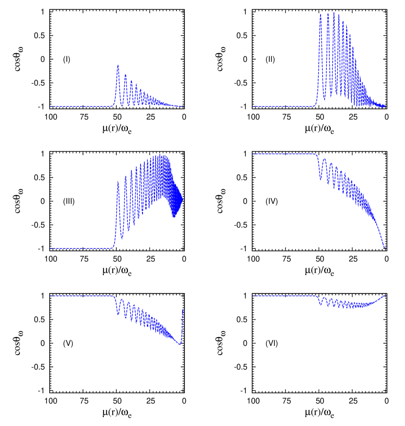
Figure 17: Example evolution of $\cos\theta_{\omega}$ as a function of $\mu(r)/\omega_{e}$ for the system shown in Figs. 1 and 2 for $2\omega/\delta m^{2}=-0.90$ (I), $-0.50$ (II), $-0.32$ (III), 0.02 (IV), 0.14 (V), and 0.50 (VI) MeV^-1, respectively. Note the similarity to the evolution shown in Figs. 14 and 15 for the six ranges of $\omega$ based on occurrences of precession-driven and nutation-driven resonances.

Next we consider the flavor evolution of the system exhibiting the spectral swaps in Figs. 1 and 2 by relaxing the single-angle approximation used to produce these results. In the so-called “multi-angle” approximation, neutrinos are emitted from the neutrino sphere with equal probability in the forward directions, which are defined to be $0\leq\theta_{\rm em}\leq\pi/2$. Here $\theta_{\rm em}$ is the angle with respect to the radial direction at the point of emission. Under the multi-angle approximation, an NFIS can be specified by the corresponding neutrino energy and emission angle in terms of $\omega$ and $\epsilon\equiv\cos\theta_{\rm em}$. The evolution of $\mathbf{s}_{\omega,\epsilon}$ is governed by

$$\frac{d}{dr}\mathbf{s}_{\omega,\epsilon}=\mathbf{s}_{\omega,\epsilon}\times\left\{\frac{\omega}{D_{\epsilon}(r)}\mathbf{H}_{\rm v}-2\mu(R_{\nu})\frac{R_{\nu}^{2}}{r^{2}}\int_{-\infty}^{\infty}g(\omega^{\prime})d\omega^{\prime}\int_{0}^{1}\mathbf{s}_{\omega^{\prime},\epsilon^{\prime}}\left[\frac{1}{D_{\epsilon}(r)D_{\epsilon^{\prime}}(r)}-1\right]\epsilon^{\prime}d\epsilon^{\prime}\right\},$$ (62)

where $\mu(R_{\nu})=2\sqrt{2}G_{F}n_{\nu_{e}}(R_{\nu})$, $n_{\nu_{e}}(R_{\nu})$ is given by Eq. (4) for $r=R_{\nu}$, and

$$D_{\epsilon}(r)\equiv\sqrt{1-(1-\epsilon^{2})R_{\nu}^{2}/r^{2}}.$$ (63)

Equation (62) reduces to Eq. (7) under the single-angle approximation that $\mathbf{s}_{\omega,\epsilon}(r)=\mathbf{s}_{\omega,\epsilon=1}(r)$.

Using the same neutrino emission parameters as for Figs. 1 and 2, we follow the flavor evolution of the system with initial number densities of $\nu_{e}$ and $\bar{\nu}_{e}$ significantly larger than those of $\nu_{x}$ and $\bar{\nu}_{x}$ under the multi-angle approximation. The angle-averaged swap factor $\langle f_{S}(\omega,\epsilon,r)\rangle_{\epsilon}$ at $r=r_{f}=250$ km is shown as a function of $2\omega/\delta m^{2}$ in Fig. 18a. This average factor is defined as

$$\langle f_{S}(\omega,\epsilon,r)\rangle_{\epsilon}\equiv\frac{\int_{0}^{1}f_{S}(\omega,\epsilon,r)[\epsilon/D_{\epsilon}(r)]d\epsilon}{\int_{0}^{1}[\epsilon/D_{\epsilon}(r)]d\epsilon}=\frac{\int_{0}^{1}f_{S}(\omega,\epsilon,r)[\epsilon/D_{\epsilon}(r)]d\epsilon}{\left[1-\sqrt{1-R_{\nu}^{2}/r^{2}}\right]r^{2}/R_{\nu}^{2}},$$ (64)

and can be used to calculate the effect of flavor transformation on e.g., neutrino reaction rates at radius $r$. Compared with the swap factor shown in Fig. 2 for the single-angle approximation, $\langle f_{S}(\omega,\epsilon,r_{f})\rangle_{\epsilon}$ is identical for $\omega>0$ but shows large deviations for $\omega<0$. On the other hand, swap factors $f_{S}(\omega,\epsilon,r_{f})$ for specific values of $\epsilon$ shown in Fig. 18b have the same general structure as shown in Fig. 2. This can be understood from the precession-driven resonance as discussed below.

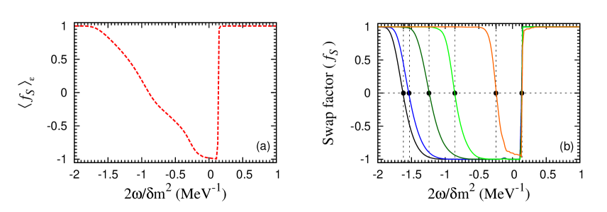
Figure 18: Angle-averaged swap factor $\langle f_{S}(\omega,\epsilon,r_{f})\rangle_{\epsilon}$ (a) and angle-specific swap factors $f_{S}(\omega,\epsilon,r_{f})$ (b) at $r_{f}=250$ km for the system with the same neutrino emission parameters as for Fig. 2 but in multi-angle approximation. From left to right, the curves for $\omega<0$ in (b) are for $\epsilon=10^{-3}$, 0.24, 0.49, 0.74, and 0.99, respectively. The sharp changes in $f_{S}(\omega,\epsilon,r_{f})$ occur at $2\omega/\delta m^{2}=-1.63$, $-1.54$, $-1.24$, $-0.86$, $-0.24$, and 0.14 MeV^-1, respectively, for which $f_{S}(\omega,\epsilon,r_{f})=0$ (filled circles).

It is convenient to define

$$\mathbf{S}_{a}\equiv \int_{-\infty}^{\infty}g(\omega)d\omega\int_{0}^{1}\mathbf{s}_{\omega,\epsilon}\epsilon d\epsilon,$$ (65a)

$$\mathbf{S}_{b}\equiv \int_{-\infty}^{\infty}g(\omega)d\omega\int_{0}^{1}\mathbf{s}_{\omega,\epsilon}\left[\frac{\epsilon}{D_{\epsilon}(r)}\right]d\epsilon,$$ (65b)

and rewrite Eq. (62) as

$$\frac{d}{dr}\mathbf{s}_{\omega,\epsilon}=\mathbf{s}_{\omega,\epsilon}\times\left\{\frac{\omega}{D_{\epsilon}(r)}\mathbf{H}_{\rm v}-2\mu(R_{\nu})\frac{R_{\nu}^{2}}{r^{2}}\left[\frac{\mathbf{S}_{b}}{D_{\epsilon}(r)}-\mathbf{S}_{a}\right]\right\}.$$ (66)

Our numerical results show that both $\mathbf{S}_{a}$ and $\mathbf{S}_{b}$ precess around $\mathbf{H}_{\rm v}$ with the same frequency $\dot{\phi}_{p}(r)$ at a specific $r$ for $R_{\nu}\leq r\lesssim r_{f}$. This is consistent with the conclusions of Duan et al. (2009) based on symmetry arguments. The synchronized oscillations of $S_{a,x}/S_{a,\perp}$ and $S_{b,x}/S_{b,\perp}$ due to precession are shown for $r=60$–80 and 200–250 km in Figs. 19a and b, respectively. Here the $x$-axis is in the plane perpendicular to $\mathbf{H}_{\rm v}$ and the subscript “$\perp$” denotes the net perpendicular component. It can be shown from Eq. (66) that $S_{a,z}\equiv\mathbf{S}_{a}\cdot\mathbf{\hat{e}}_{z}^{\rm I}$ ($\mathbf{\hat{e}}_{z}^{\rm I}=-\mathbf{H}_{\rm v}$) is conserved (see Fig. 20a). Components of the “mean field” $\mathbf{S}_{b}/D_{\epsilon}(r)-\mathbf{S}_{a}$ are shown as functions of $r$ for $\epsilon=0$ (solid curve) and 1 (dashed curve) in Figs. 20b and c. Clearly, the mean field experienced by $\mathbf{s}_{\omega,\epsilon}$ is different for different $\epsilon$. It can also be seen from Fig. 20c that the perpendicular component $S_{b,\perp}/D_{\epsilon}(r)-S_{a,\perp}$ increases sharply at $r_{\rm cr}\approx 64$ km just as $S_{\perp}$ does at the critical point in the single-angle approximation (see Fig. 4). However, in contrast to the single-angle approximation, nutation of the mean field is damped out very quickly in the multi-angle approximation, and therefore, can be neglected.

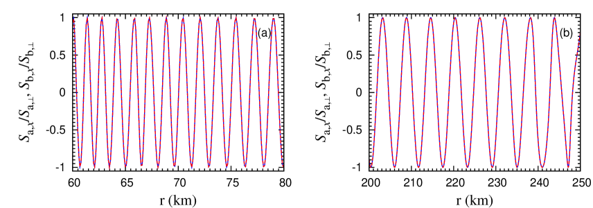
Figure 19: Synchronized oscillations of $S_{a,x}/S_{a,\perp}$ and $S_{b,x}/S_{b,\perp}$ due to precession for the system shown in Fig. 18 for $r=60$–80 (a) and 200–250 km (b). In either panel two curves are shown but they are indistinguishable.

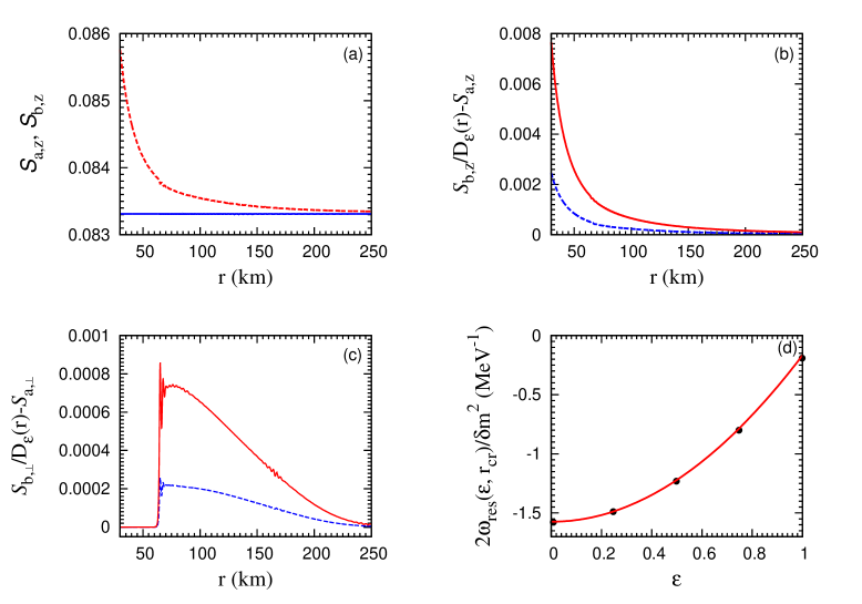
Figure 20: Components of the mean field as functions of $r$: (a) $S_{a,z}$ (solid curve) and $S_{b,z}$ (dashed curve), (b) $S_{b,z}/D_{\epsilon}(r)-S_{a,z}$ for $\epsilon=0$ (solid curve) and 1 (dashed curve), and (c) $S_{b,\perp}/D_{\epsilon}(r)-S_{a,\perp}$ for $\epsilon=0$ (solid curve) and 1 (dashed curve). (d) The value of $2\omega_{\rm res}(\epsilon,r_{\rm cr})/\delta m^{2}$ at $r_{\rm cr}\approx 64$ km shown as a function of $\epsilon$. From left to right, the filled circles correspond to $2\omega_{\rm res}(\epsilon,r_{\rm cr})/\delta m^{2}\approx-1.57$, $-1.50$, $-1.24$, $-0.81$, and $-0.21$ MeV^-1, respectively. These values are very close to those values of $2\omega/\delta m^{2}$ that correspond to the filled circles at $\omega<0$ in Fig. 18b.

Based on the above discussion, we only need to consider the precession-driven resonance in explaining the swap factor $f_{S}(\omega,\epsilon,r_{f})$. A precession-driven resonance occurs when the $z$-component of the net effective field interacting with $\mathbf{s}_{\omega,\epsilon}$ vanishes in the co-precessing frame (see Sec. IV.1). It can be seen from Eq. (66) that $\mathbf{s}_{\omega,\epsilon}$ goes through a precession-driven resonance when

$$\omega=\omega_{\rm res}(\epsilon,r)\equiv D_{\epsilon}(r)\left\{\dot{\phi}_{p}(r)-2\mu(R_{\nu})\frac{R_{\nu}^{2}}{r^{2}}\left[\frac{S_{b,z}}{D_{\epsilon}(r)}-S_{a,z}\right]\right\}.$$ (67)

However, evolution through a resonance at $r<r_{\rm cr}$ is extremely non-adiabatic and does not result in any net flavor transformation. Thus, we expect that net full conversion [$f_{S}(\omega,\epsilon,r_{f})=-1$] occurs only for $\omega_{\rm res}(\epsilon,r_{\rm cr})<\omega<\omega_{\rm res}(\epsilon,r_{f})$. At $r=r_{\rm cr}$, $\omega_{\rm res}(\epsilon,r_{\rm cr})<0$ for $0\leq\epsilon\leq 1$ and is larger for a larger $\epsilon$ (more radial trajectory, see Fig. 20d). At $r=r_{f}$, $D_{\epsilon}(r)\approx 1$ and $S_{b,z}/D_{\epsilon}(r)-S_{a,z}$ becomes very small (see Fig. 20b), so $\omega_{\rm res}(\epsilon,r_{f})\approx\dot{\phi}_{p}(r_{f})$ and is nearly independent of $\epsilon$. Using our numerical results for $\dot{\phi}_{p}(r)$, $S_{a,z}$, and $S_{b,z}$, we obtain ${2\omega_{\rm res}(\epsilon,r_{\rm cr})}/{\delta m^{2}}\approx-1.57$, $-1.50$, $-1.24$, $-0.81$, and $-0.21$ MeV^-1 for $\epsilon=10^{-3}$, 0.24, 0.49, 0.74, and 0.99, respectively, and ${2\omega_{\rm res}(\epsilon,r_{f})}/{\delta m^{2}}\approx 0.14$ MeV^-1 for $0\leq\epsilon\leq 1$. These results are in excellent agreement with Figure 18b.

VI Conclusions

Using a system initially consisting of $\nu_{e}$ and $\bar{\nu}_{e}$ with the same energy spectrum but different number densities, we have shown that flavor evolution of this system in the single-angle approximation can be understood in terms of the response of individual NFIS’s to the mean field, which is very well approximated by the total angular momentum of a neutrino gyroscope. The evolution of an NFIS is governed by two types of resonances driven by precession and nutation of the gyroscope, respectively. A resonance does not affect the net flavor transformation if evolution through it is extremely non-adiabatic. Nearly full flavor conversion occurs following adiabatic evolution through an odd number of resonances but there is no net flavor transformation following adiabatic evolution through an even number (including zero) of resonances. The detailed results on NFIS evolution are presented in Figs. 14, 15, and 16, and discussed in Secs. IV.3 and IV.4.

We have also shown that the above results for the system of two initial neutrino species can be extended to a system of four species with the initial number densities of $\nu_{e}$ and $\bar{\nu}_{e}$ significantly larger than those of $\nu_{x}$ and $\bar{\nu}_{x}$. Further, we find that when the multi-angle approximation is adopted instead of the single-angle approximation, nutation of the mean field is quickly damped out and can be neglected. In contrast, precession-driven resonances still govern the evolution of NFIS’s with different energy and emission angles just as in the single-angle approximation. These results are presented and discussed in Sec. V.

In conclusion, we have presented a detailed analysis of collective neutrino oscillations in supernovae for the case where the initial number densities of $\nu_{e}$ and $\bar{\nu}_{e}$ are significantly larger than those of $\nu_{x}$ and $\bar{\nu}_{x}$. We note that some earlier works (e.g., Raffelt and Smirnov (2007b)) and two recent studies Raffelt (2011); Galais and Volpe (2011) have similar goals to ours but used very different methods. Our approach is mostly pedagogical and analytic. It is our hope that along with other parallel efforts, we have provided some insights into the seemingly complicated yet fascinating phenomena of collective neutrino oscillations.

Appendix A Parameters of the Neutrino Gyroscope at a specific $\mu$

In addition to the procedure given in Sec. III.2, the parameters of the neutrino gyroscope at a specific $\mu$ can be obtained using the “pure-precession” ansatz (see also discussion in Duan et al. (2007)), which assumes that $\mathbf{s}_{1}$ and $\mathbf{s}_{2}$ associated with the gyroscope always stay in the same plane as $\mathbf{H}_{\rm v}=-\mathbf{\hat{e}}_{z}^{\rm I}$ and precess with the same angular velocity $\dot{\phi}_{p}\mathbf{\hat{e}}_{z}^{\rm I}$. More specifically, we can use the Euler angles in Frame I to write

$$\mathbf{s}_{1} =\frac{1}{2}(\sin\theta_{1}\sin\phi_{1}\mathbf{\hat{e}}_{x}^{\rm I}-\sin\theta_{1}\cos\phi_{1}\mathbf{\hat{e}}_{y}^{\rm I}+\cos\theta_{1}\mathbf{\hat{e}}_{z}^{\rm I}),$$ (68a)

$$\mathbf{s}_{2} =\frac{1}{2}(\sin\theta_{2}\sin\phi_{2}\mathbf{\hat{e}}_{x}^{\rm I}-\sin\theta_{2}\cos\phi_{2}\mathbf{\hat{e}}_{y}^{\rm I}+\cos\theta_{2}\mathbf{\hat{e}}_{z}^{\rm I}).$$ (68b)

The ansatz assumes that $\dot{\theta}_{1}=\dot{\theta}_{2}=0$, $\dot{\phi}_{1}=\dot{\phi}_{2}=\dot{\phi}_{p}$, and $\phi_{2}-\phi_{1}=\pi$ (the last relation can be seen from the initial configuration at the neutrino sphere with $\mathbf{s}_{1}=-\mathbf{s}_{2}=\mathbf{\hat{e}}_{z}^{\rm f}/2$ corresponding to $\theta_{1}=2\tilde{\theta}_{\rm v}$ and $\theta_{2}=\pi-2\tilde{\theta}_{\rm v}$). Using this ansatz along with conservation of $S_{z}$ and Eqs. (20a) and (20b), we obtain

$$\cos\theta_{1}+\alpha\cos\theta_{2} =(1-\alpha)\cos 2\tilde{\theta}_{\rm v},$$ (69a)

$$\dot{\phi}_{p}\sin\theta_{1} =\mu_{\rm v}\sin\theta_{1}+\frac{\alpha\mu}{2}\sin(\theta_{1}+\theta_{2}),$$ (69b)

$$\dot{\phi}_{p}\sin\theta_{2} =-\mu_{\rm v}\sin\theta_{2}+\frac{\mu}{2}\sin(\theta_{1}+\theta_{2}).$$ (69c)

For any specific $\mu$, the above equations can be solved to give $\theta_{1}$, $\theta_{2}$, and $\dot{\phi}_{p}$. Then we can calculate the corresponding $\sigma$, $Q$, and $\theta_{p}$ using $\theta_{1}$ and $\theta_{2}$. The above procedure gives $\sigma$, $Q$, $\theta_{p}$, and $\dot{\phi}_{p}$ for the gyroscope at a specific $\mu$ that are indistinguishable from those obtained by the procedure discussed in Sec. III.2.

Appendix B Initial Conditions for the Neutrino Gyroscope

The initial conditions for the neutrino gyroscope at the neutrino sphere are

$$\mathbf{S}(0) =\frac{1-\alpha}{2}\mathbf{\hat{e}}_{z}^{\rm f},$$ (70a)

$$\mathbf{Q}(0) =\frac{1+\alpha}{2}\mathbf{\hat{e}}_{z}^{\rm f}+\frac{\mu_{\rm v}}{\mu}\mathbf{H}_{\rm v}.$$ (70b)

Noting that $\mathbf{H}_{\rm v}=-\sin 2\tilde{\theta}_{\rm v}\mathbf{\hat{e}}_{x}^{\rm f}-\cos 2\tilde{\theta}_{\rm v}\mathbf{\hat{e}}_{z}^{\rm f}=-\mathbf{\hat{e}}_{z}^{\rm I}$, we obtain from the above equations

$$S_{z} =\frac{1-\alpha}{2}\cos 2\tilde{\theta}_{\rm v},$$ (71a)

$$Q =\left[\left(\frac{1+\alpha}{2}-\frac{\mu_{\rm v}}{\mu}\cos 2\tilde{\theta}_{\rm v}\right)^{2}+\left(\frac{\mu_{\rm v}}{\mu}\sin 2\tilde{\theta}_{\rm v}\right)^{2}\right]^{1/2},$$ (71b)

$$\sigma =\frac{1-\alpha}{2Q}\left(\frac{1+\alpha}{2}-\frac{\mu_{\rm v}}{\mu}\cos 2\tilde{\theta}_{\rm v}\right).$$ (71c)

In terms of the dynamic variables $\theta$ and $\phi$, the initial conditions for the neutrino gyroscope can be chosen as $\dot{\theta}_{0}=0$, $\phi_{0}=0$, and

$$\cos\theta_{0} =\frac{1}{Q}\left(\frac{1+\alpha}{2}\cos 2\tilde{\theta}_{\rm v}-\frac{\mu_{\rm v}}{\mu}\right),$$ (72a)

$$\dot{\phi}_{0} =\mu_{\rm v}\frac{1-\alpha}{1+\alpha},$$ (72b)

where the subscript “0” indicates the initial moment $t=0$ and Eq. (72b) is obtained from Eq. (21a) at $t=0$. For a constant $\mu$, the precession frequency at $\theta=\theta_{p}$, where $V_{\rm eff}(\theta)$ reaches its minimum, is given by Eq. (31) as

$$\dot{\phi}_{p}=\frac{\mu\sigma\pm\sqrt{(\mu\sigma)^{2}-4\mu\mu_{\rm v}Q\cos\theta_{p}}}{2\cos\theta_{p}}\approx\begin{cases}(\mu\sigma/\cos\theta_{p})-(\mu_{\rm v}Q/\sigma),\\ \mu_{\rm v}Q/\sigma,\end{cases}$$ (73)

where the approximate equalities apply for $\mu_{\rm v}/\mu\ll 1$ with the upper and lower expressions corresponding to the plus and minus signs in front of the square root, respectively. It can be shown that the upper expression of $\dot{\phi}_{p}$ is unphysical as it cannot satisfy conservation of $S_{z}$. For the physical value of $\dot{\phi}_{p}\approx\mu_{\rm v}Q/\sigma$, conservation of $S_{z}$ gives

$$\theta_{p}\approx 2\tilde{\theta}_{\rm v}\left[1+\frac{2(1+\alpha)}{(1-\alpha)^{2}}\frac{\mu_{\rm v}}{\mu}\right].$$ (74)

The above expression of $\theta_{p}$ is to the first order in $\mu_{\rm v}/\mu$ and $\tilde{\theta}_{\rm v}$. To the same order, we have

$$\theta_{0}\approx 2\tilde{\theta}_{\rm v}\left(1+\frac{2}{1+\alpha}\frac{\mu_{\rm v}}{\mu}\right).$$ (75)

The amplitude of nutation around $\theta=\theta_{p}$ is then

$$\eta=\theta_{p}-\theta_{0}\approx\frac{16\alpha\tilde{\theta}_{\rm v}}{(1+\alpha)(1-\alpha)^{2}}\frac{\mu_{\rm v}}{\mu}.$$ (76)

The number density of $\nu_{e}$ at the neutrino sphere is

$$n_{\nu_{e}}(R_{\nu})=\frac{L_{\nu_{e}}}{4\pi R_{\nu}^{2}\langle E_{\nu_{e}}\rangle}=1.66\times 10^{32}\left(\frac{L_{\nu_{e}}}{10^{51}\ {\rm erg/s}}\right)\left(\frac{10\ {\rm km}}{R_{\nu}}\right)^{2}\left(\frac{10\ {\rm MeV}}{\langle E_{\nu_{e}}\rangle}\right)\ {\rm cm}^{-3}.$$ (77)

For $\mu=2\sqrt{2}G_{F}n_{\nu_{e}}(R_{\nu})$,

$$\frac{\mu_{\rm v}}{\mu}=5.92\times 10^{-6}\left(\frac{\delta m^{2}}{3\times 10^{-3}\ {\rm eV}^{2}}\right)\left(\frac{10\,{\rm MeV}}{E}\right)\left[\frac{10^{32}\ {\rm cm}^{-3}}{n_{\nu_{e}}(R_{\nu})}\right].$$ (78)

Taking $\tilde{\theta}_{\rm v}=10^{-5}$, $\delta m^{2}=3\times 10^{-3}$ eV², $2\mu_{\rm v}/\delta m^{2}=1/9$ MeV^-1, $\alpha=2/3$, and $n_{\nu_{e}}(R_{\nu})=1.66\times 10^{32}$ cm^-3, we have $\eta\approx 2.28\times 10^{-9}$.

Appendix C The Neutrino Gyroscope at the Critical Point

The critical point at $\mu=\mu_{\rm cr}$ separates the evolution of the neutrino gyroscope into two regimes: the sleeping-top regime with essentially pure precession but little nutation at $\mu\gtrsim\mu_{\rm cr}$ and the other with both precession and nutation at $\mu<\mu_{\rm cr}$. As $\theta\ll 1$ in the sleeping-top regime, we derive $\mu_{\rm cr}$ assuming $\tilde{\theta}_{\rm v}=0$. Let the gyroscope start with $\theta=0$ at a constant $\mu$. Its fixed parameters are

$$S_{z} =\sigma=\frac{1-\alpha}{2},$$ (79a)

$$Q =\frac{1+\alpha}{2}-\frac{\mu_{\rm v}}{\mu},$$ (79b)

$$E_{\rm gyro} =\frac{\mu}{2}\sigma^{2}+\mu_{\rm v}Q.$$ (79c)

The motion of the gyroscope is governed by

$$\frac{\dot{\phi}}{\mu}\sin^{2}\theta =\sigma(1-\cos\theta),$$ (80a)

$$\frac{1}{2\mu}(\dot{\theta}^{2}+\dot{\phi}^{2}\sin^{2}\theta) =\mu_{\rm v}Q(1-\cos\theta),$$ (80b)

which are obtained by rewriting Eqs. (25c) and (26b). Assuming that $\theta>0$ is allowed, we can find $\theta_{\rm max}$, the maximum value of $\theta$, by setting $\dot{\theta}=0$ in Eq. (80b). Combining the resulting equation with Eq. (80a), we obtain

$$\cos\theta_{\rm max}=\frac{\mu\sigma^{2}}{2\mu_{\rm v}Q}-1.$$ (81)

It can be seen that when $\mu\sigma^{2}\geq 4\mu_{\rm v}Q$, the above equation has no solution for $\theta_{\rm max}>0$. Thus, the gyroscope remains in its initial vertical position ($\theta=0$) for $\mu\sigma^{2}\geq 4\mu_{\rm v}Q$. For a gyroscope starting at $\mu\gg\mu_{\rm v}$, this condition corresponds to $\mu\geq\mu_{\rm cr}$, where

$$\mu_{\rm cr}\equiv\frac{4\mu_{\rm v}}{(1-\sqrt{\alpha})^{2}}.$$ (82)

Expanding $S_{z}=(1-\alpha)\cos 2\tilde{\theta}_{\rm v}/2$ to the leading order in $\tilde{\theta}_{\rm v}$, we obtain the pure-precession solution at $\mu=\mu_{\rm cr}$ from Eqs. (31), (37a), (38a), and (38b) (setting $\eta=0$ in the last equation):

$$\sigma_{\rm cr} \approx\sigma^{(0)}\left[1-\frac{(1-\sqrt{\alpha})^{2}}{8\sqrt{2\alpha}}\theta_{p,{\rm cr}}^{3}\right],$$ (83a)

$$Q_{\rm cr} \approx Q^{(0)}\left[1+\frac{(1-\sqrt{\alpha})^{2}}{4\sqrt{2\alpha}}\theta_{p,{\rm cr}}^{3}\right],$$ (83b)

$$\theta_{p,{\rm cr}} \approx\frac{2\sqrt{2}\alpha^{1/6}}{(1+\sqrt{\alpha})^{2/3}}\tilde{\theta}_{\rm v}^{2/3},$$ (83c)

$$\dot{\phi}_{p,{\rm cr}} \approx\dot{\phi}_{p}^{(0)}\left(1-\frac{\theta_{p,{\rm cr}}}{\sqrt{2}}+\frac{1+\alpha}{4\sqrt{2}}\theta_{p,{\rm cr}}^{2}\right),$$ (83d)

where $\sigma^{(0)}=(1-\alpha)/2$, $Q^{(0)}=(1+\alpha)/2-\mu_{\rm v}/\mu_{\rm cr}$, and $\dot{\phi}_{p}^{(0)}=\mu_{\rm cr}\sigma^{(0)}/2$. For $\alpha=2/3$ and $\tilde{\theta}_{\rm v}=10^{-5}$, we have $\theta_{p,{\rm cr}}\approx 8.24\times 10^{-4}$, which agrees with the numerical result very well. Using the above results at the critical point and Eq. (30b), we obtain

$$\omega_{n,{\rm cr}}\approx\frac{\sqrt{3}}{2}\mu_{\rm cr}\sigma^{(0)}\theta_{p,{\rm cr}}.$$ (84)

We note that the behavior of the precession and nutation frequencies at the critical point as shown in Fig. 9 is unique to the IH. In contrast, both the precession and nutation frequencies increase smoothly with $\mu$ for the NH.

References

- Nakamura et al. (2010) (Particle Data Group) K. Nakamura et al. (Particle Data Group), J. Phys. G 37, 070521 (2010).
- Wolfenstein (1978) L. Wolfenstein, Phys. Rev. D 17, 2369 (1978).
- Mikheyev and Smirnov (1985) S. P. Mikheyev and A. Y. Smirnov, Sov. J. Nucl. Phys. 42, 913 (1985).
- Duan et al. (2010) H. Duan, G. M. Fuller, and Y.-Z. Qian, Annu. Rev. Nucl. Part. Sci. 60, 569 (2010), eprint arXiv:1001.2799 [astro-ph].
- Fuller et al. (1987) G. M. Fuller, R. W. Mayle, J. R. Wilson, and D. N. Schramm, Astrophys. J. 322, 795 (1987).
- Pantaleone (1992) J. Pantaleone, Phys. Lett. B 287, 128 (1992).
- Sigl and Raffelt (1993) G. Sigl and G. G. Raffelt, Nucl. Phys. B406, 423 (1993).
- Balantekin and Yksel (2005) A. B. Balantekin and H. Yksel, New J. Phys. 7, 51 (2005), eprint astro-ph/0411159.
- Fuller and Qian (2006) G. M. Fuller and Y.-Z. Qian, Phys. Rev. D 73, 023004 (2006), eprint astro-ph/0505240.
- Duan et al. (2006a) H. Duan, G. M. Fuller, and Y.-Z. Qian, Phys. Rev. D 74, 123004 (2006a), eprint astro-ph/0511275.
- Duan et al. (2006b) H. Duan, G. M. Fuller, J. Carlson, and Y.-Z. Qian, Phys. Rev. D 74, 105014 (2006b), eprint astro-ph/0606616.
- Raffelt and Smirnov (2007a) G. G. Raffelt and A. Y. Smirnov, Phys. Rev. D 76, 081301(R) (2007a), eprint arXiv:0705.1830.
- Fogli et al. (2007) G. Fogli, E. Lisi, A. Marrone, and A. Mirizzi, JCAP 0712, 010 (2007), eprint arXiv:0707.1998.
- Dasgupta et al. (2009) B. Dasgupta, A. Dighe, G. G. Raffelt, and A. Y. Smirnov, Phys. Rev. Lett. 103, 051105 (2009), eprint arXiv:0904.3542.
- Mirizzi and Toms (2010) A. Mirizzi and R. Toms, preprint (2010), eprint arXiv:1012.1339 [hep-ph].
- Hannestad et al. (2006) S. Hannestad, G. G. Raffelt, G. Sigl, and Y. Y. Y. Wong, Phys. Rev. D 74, 105010 (2006), eprint astro-ph/0608695.
- Duan et al. (2007) H. Duan, G. M. Fuller, J. Carlson, and Y.-Z. Qian, Phys. Rev. D 75, 125005 (2007), eprint astro-ph/0703776.
- Duan et al. (2009) H. Duan, G. M. Fuller, and Y.-Z. Qian, J. Phys. G 36, 105003 (2009), eprint arXiv:0808.20 [astro-ph].
- Raffelt and Smirnov (2007b) G. G. Raffelt and A. Y. Smirnov, Phys. Rev. D 76, 125008 (2007b), eprint astro-ph/0709.4641.
- Raffelt (2011) G. G. Raffelt, preprint (2011), eprint arXiv:1103.2891 [hep-ph].
- Galais and Volpe (2011) S. Galais and C. Volpe, preprint (2011), eprint arXiv:1103.5302 [astro-ph].